Frequency-time domain combined analysis method for bidirectional wireless power transfer system based on single-stage AC-AC converter

Xi Zhang; Qianfan Zhang; Hongxing Wu; Shuai Dong; Xi Zhang; Qianfan Zhang; Hongxing Wu; Shuai Dong

doi:10.48130/wpt-0025-0032

Figures (17) Tables (5)

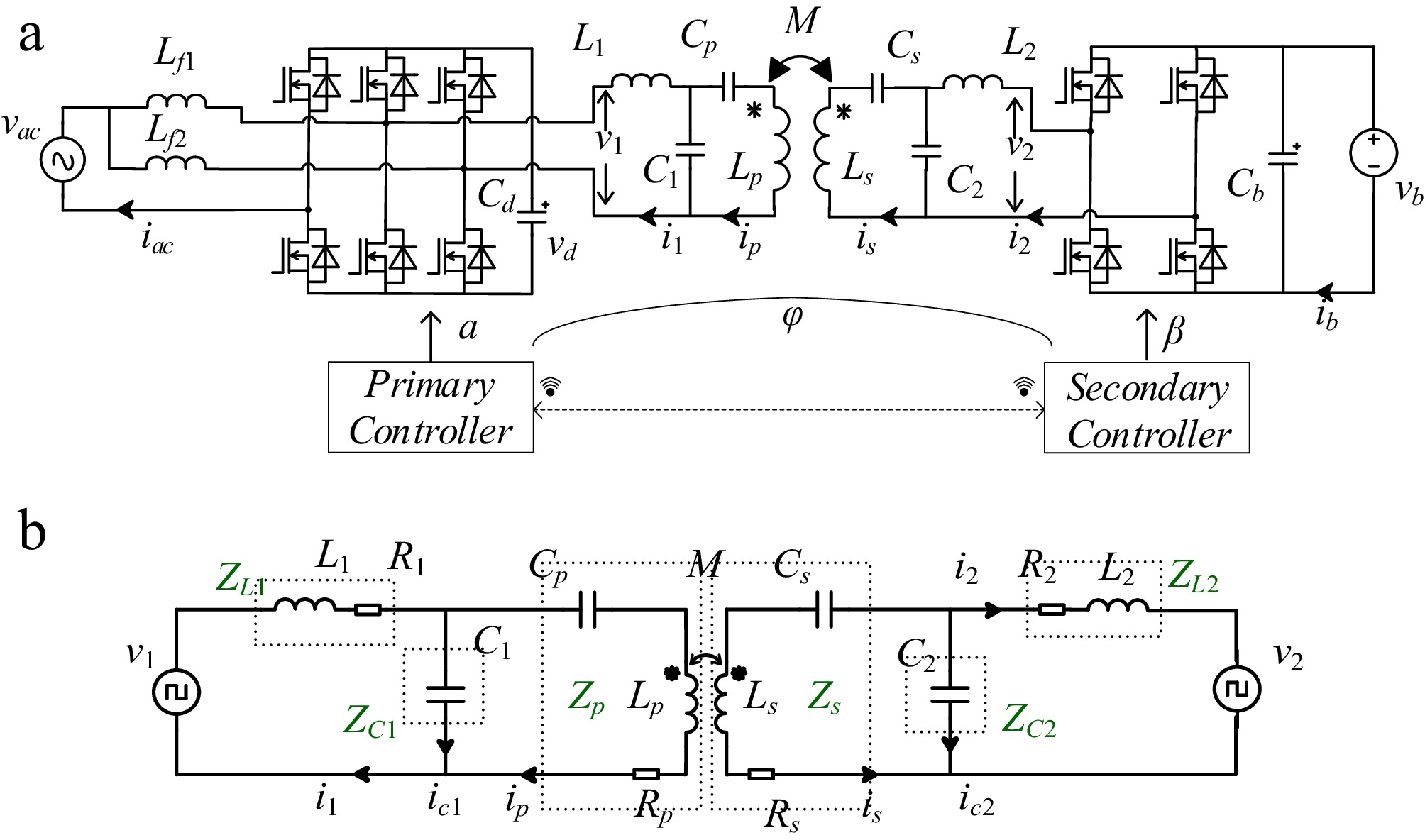
Figure 1.
Schematic of BWPT system. (a) BWPT circuit with totem converter. (b) Equivalent circuit with linear elements.
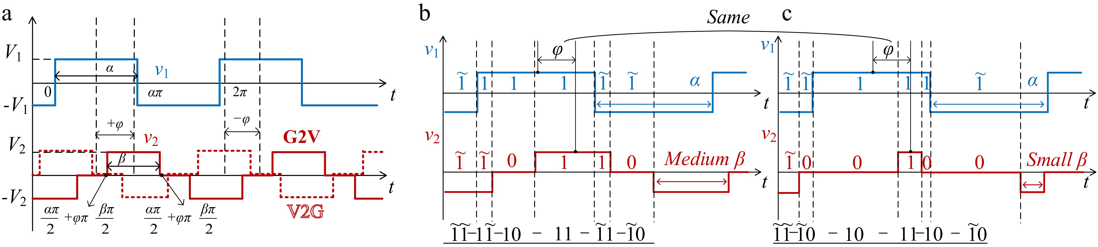
Figure 2.
Schematic of transmitter and receiver side voltage phase shift. (a) Bidirectional voltage phase delay schematic. (b) Medium β for the system. (c) Small β for the system.
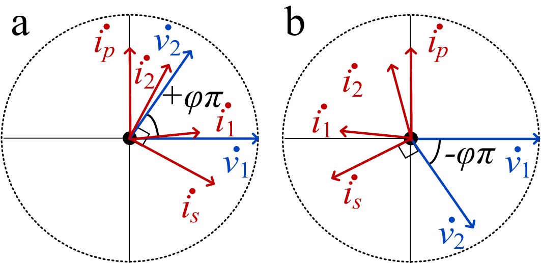
Figure 3.
Schematic diagram of voltage and current phases in a passive network. (a) G2V. (b) V2G.
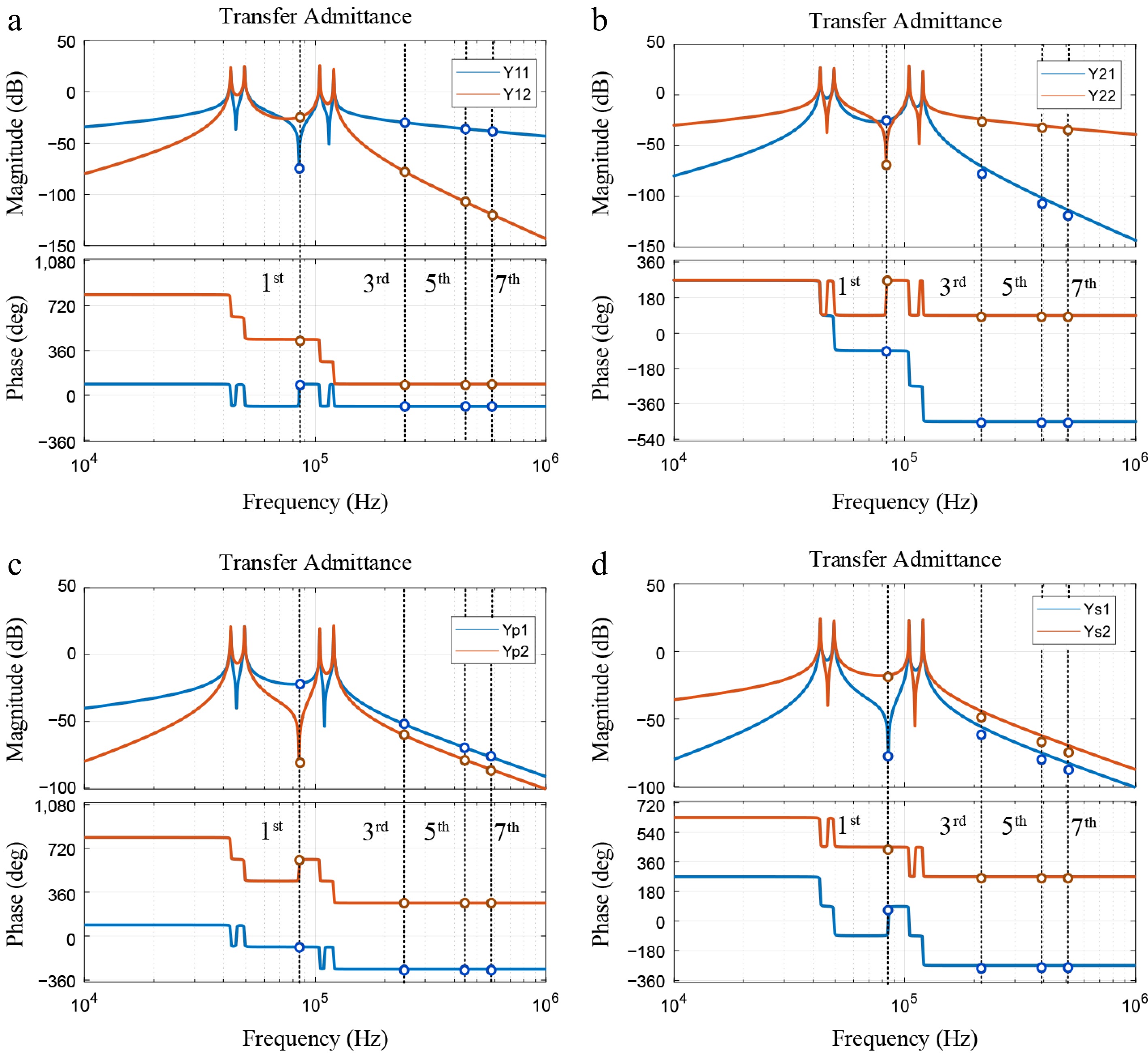
Figure 4.
Coefficient admittance matrix amplitude-phase characteristic diagram. (a) Y₁₁ and Y₁₂. (b) Y₂₁ and Y₂₂. (c) Y_p1 and Y_p2. (d) Y_s1 and Y_s2.
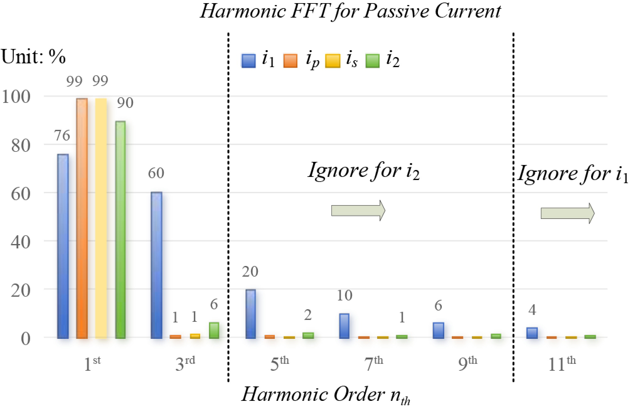
Figure 5.
Schematic diagram of the harmonics composition of each current.
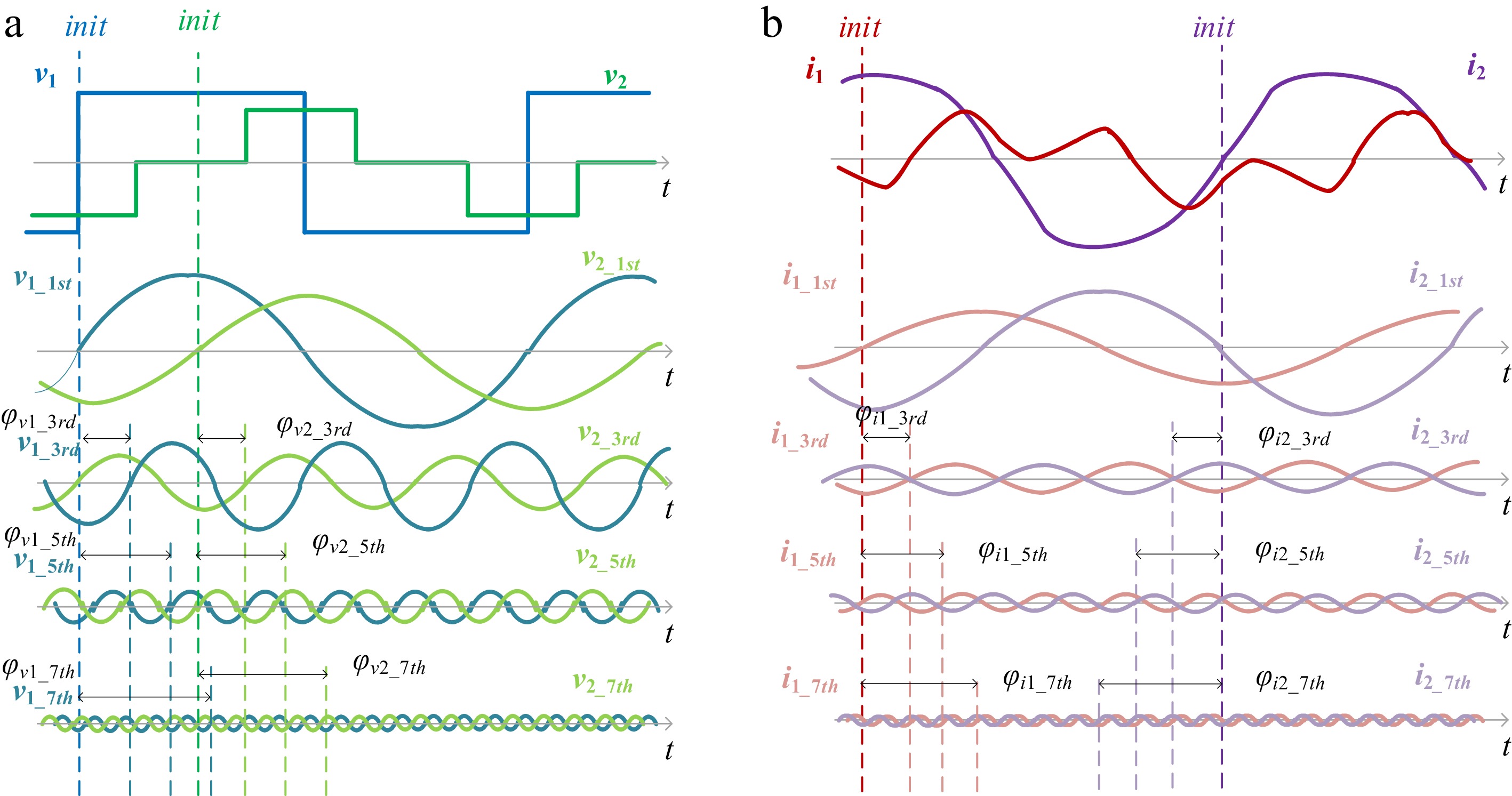
Figure 6.
Phase correction for passive network voltage and current. (a) Voltage v₁ and v₂. (b) Current i₁ and i₂.
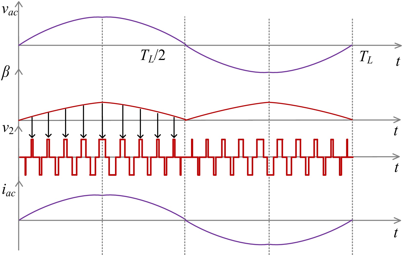
Figure 7.
Waveforms of PFC control using the β regulation method.
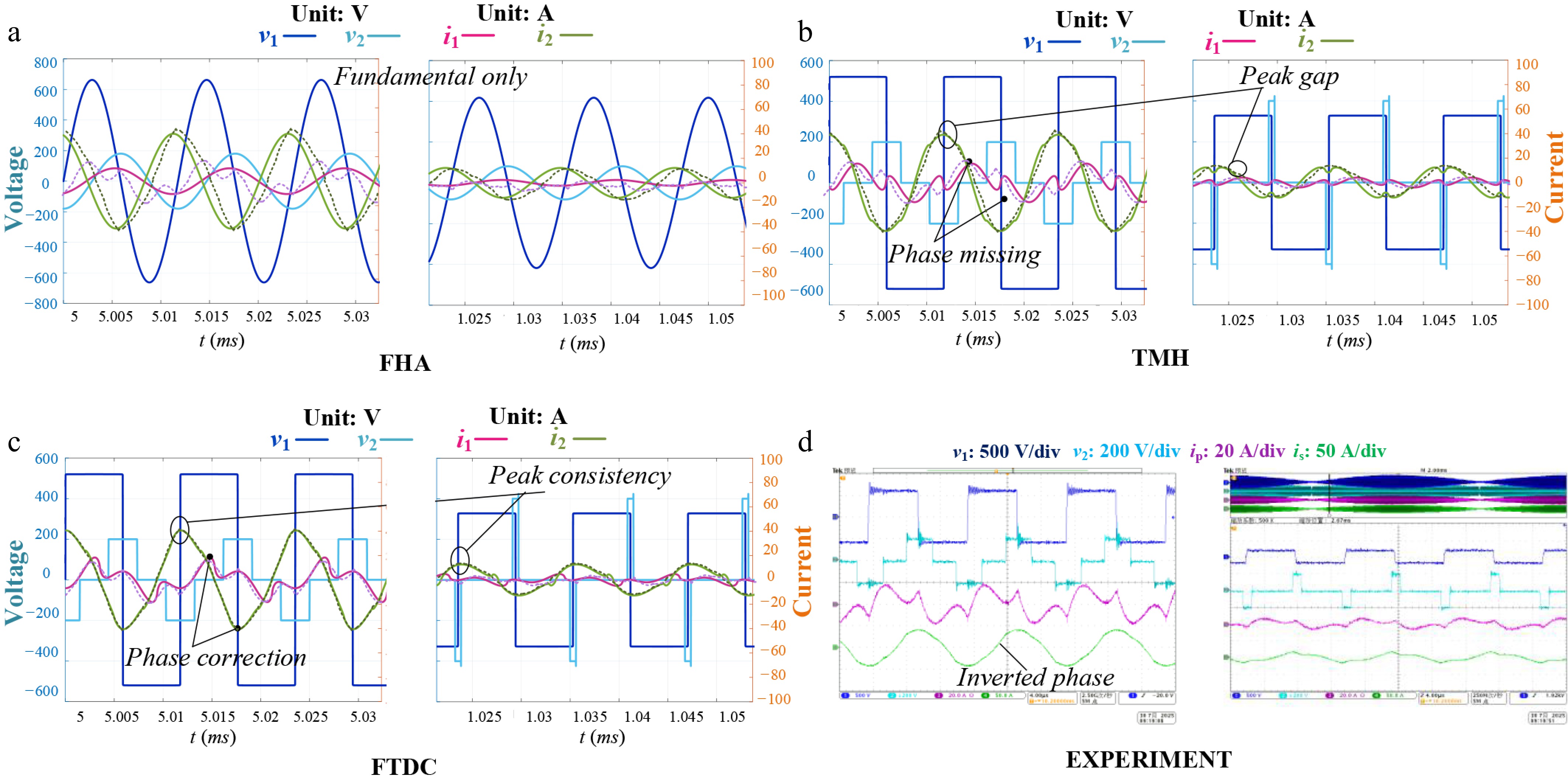
Figure 8.
Theory derivation comparison under φ = 0.5 for G2V (left: max grid voltage v_ac; right: low grid voltage v_ac). (a) FHA. (b) TMH. (c) FTDC. (d) Experiment.
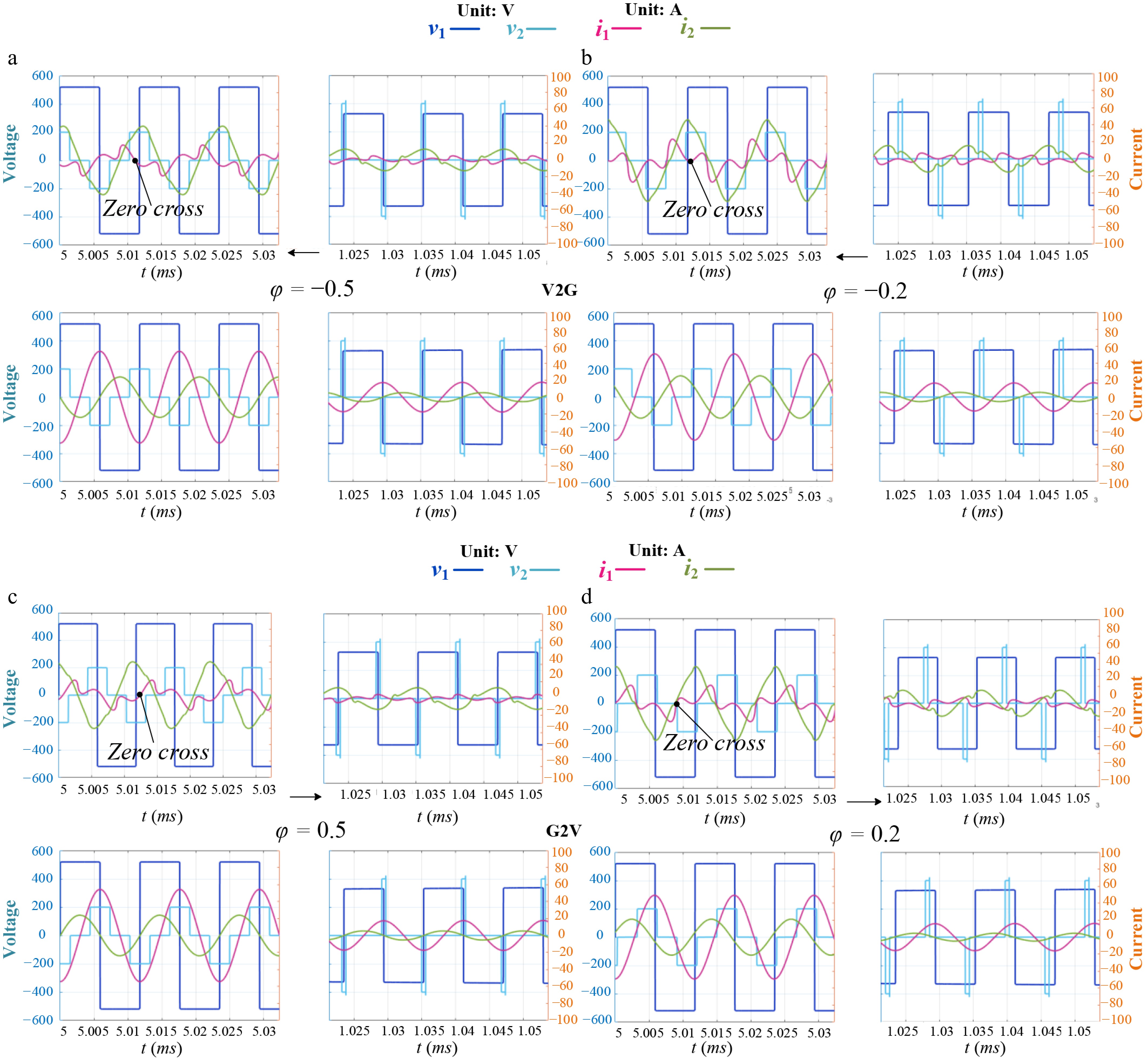
Figure 9.
Theory derivation of voltage and current in steady state (left: max v_ac; right: low v_ac). (a) φ = −0.5 for V2G. (b) φ = −0.2 for V2G. (c) φ = 0.5 for G2V. (d) φ = 0.2 for G2V.
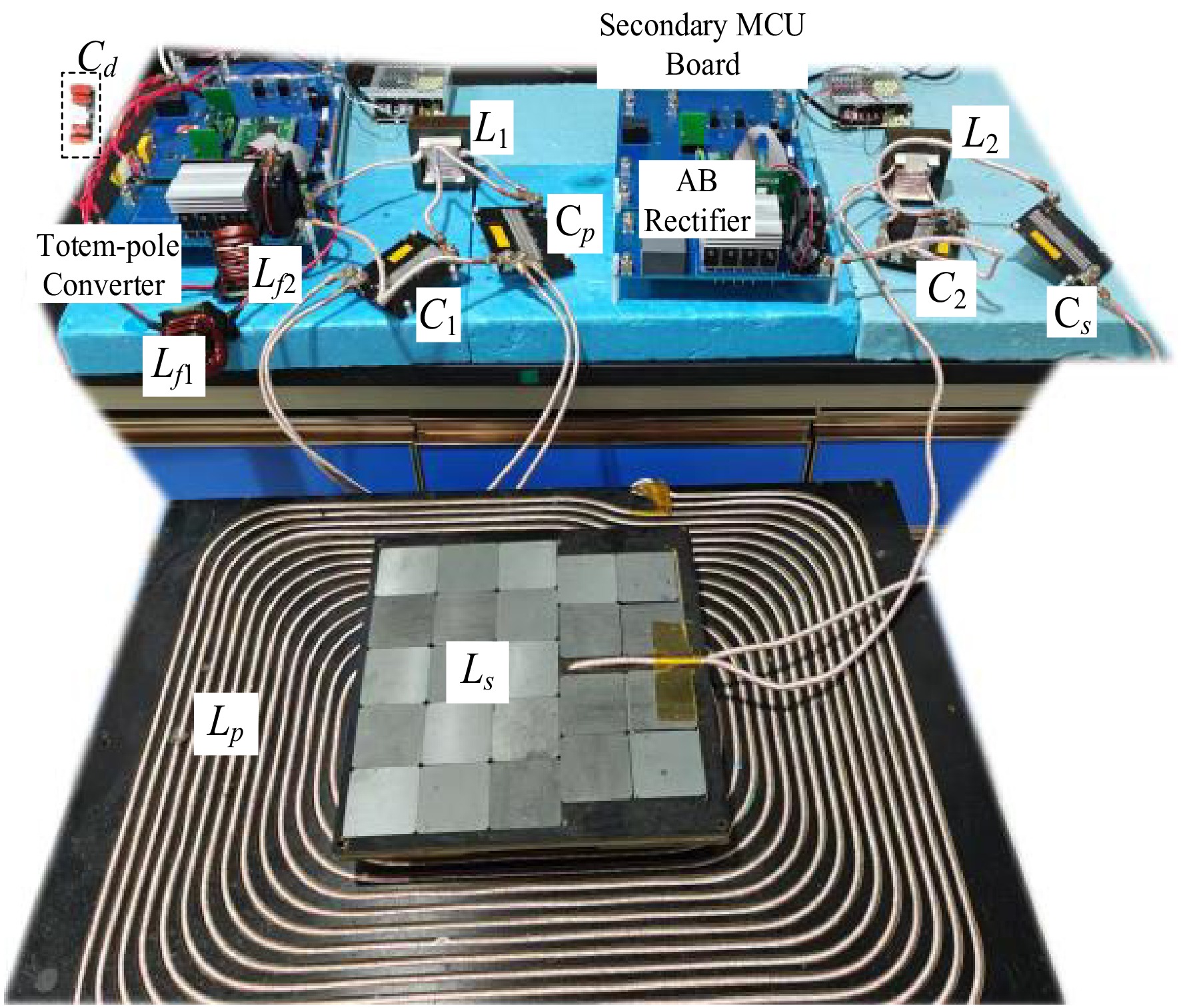
Figure 10.
BWPT system experiment test bench.
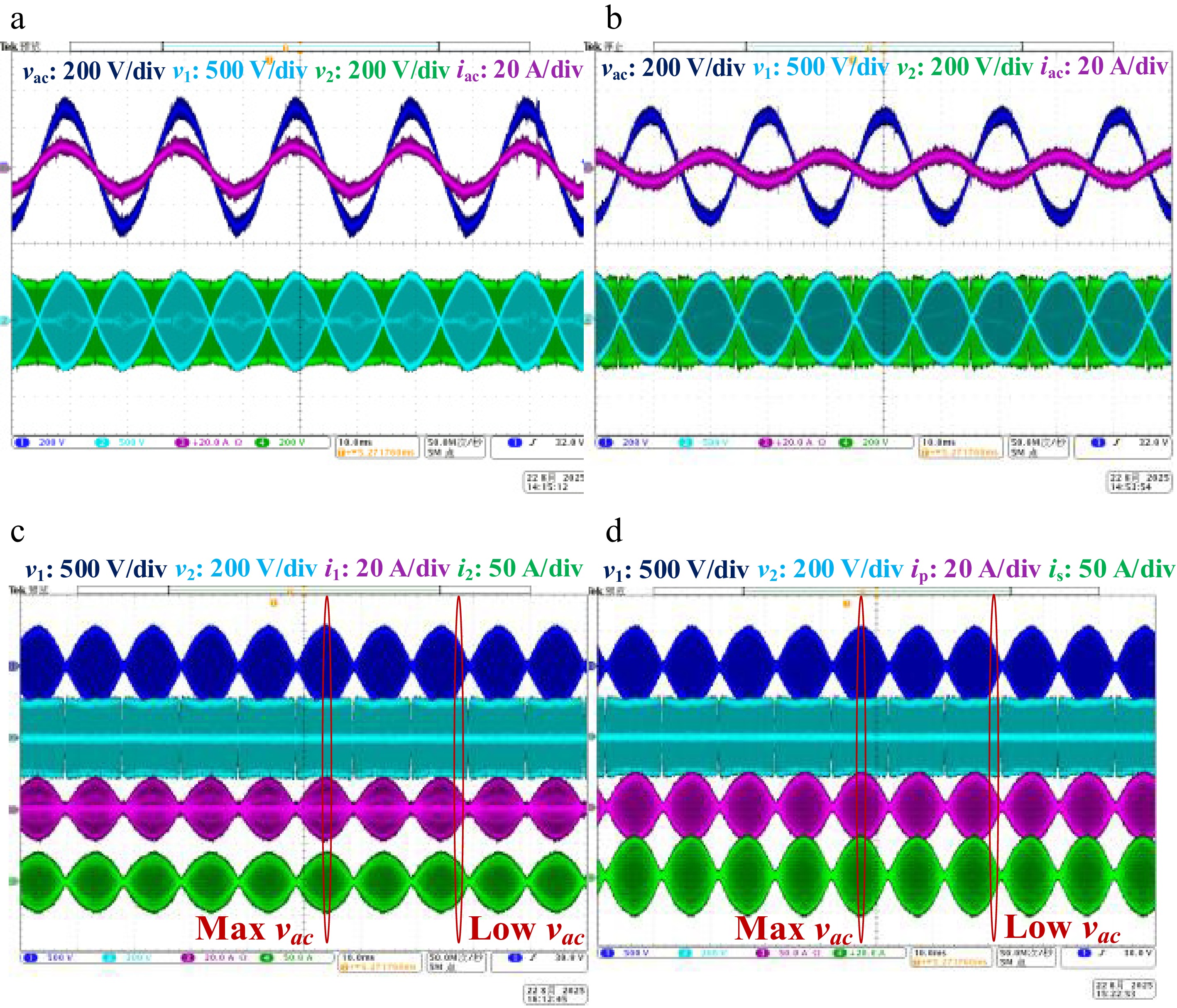
Figure 11.
Specific experiment waveforms of BWPT system. (a) φ = 0.5 for G2V. (b) φ = −0.3 for V2G. (c) Steady-state waveforms with i₁ and i₂. (d) Steady-state waveforms with i_p and i_s.
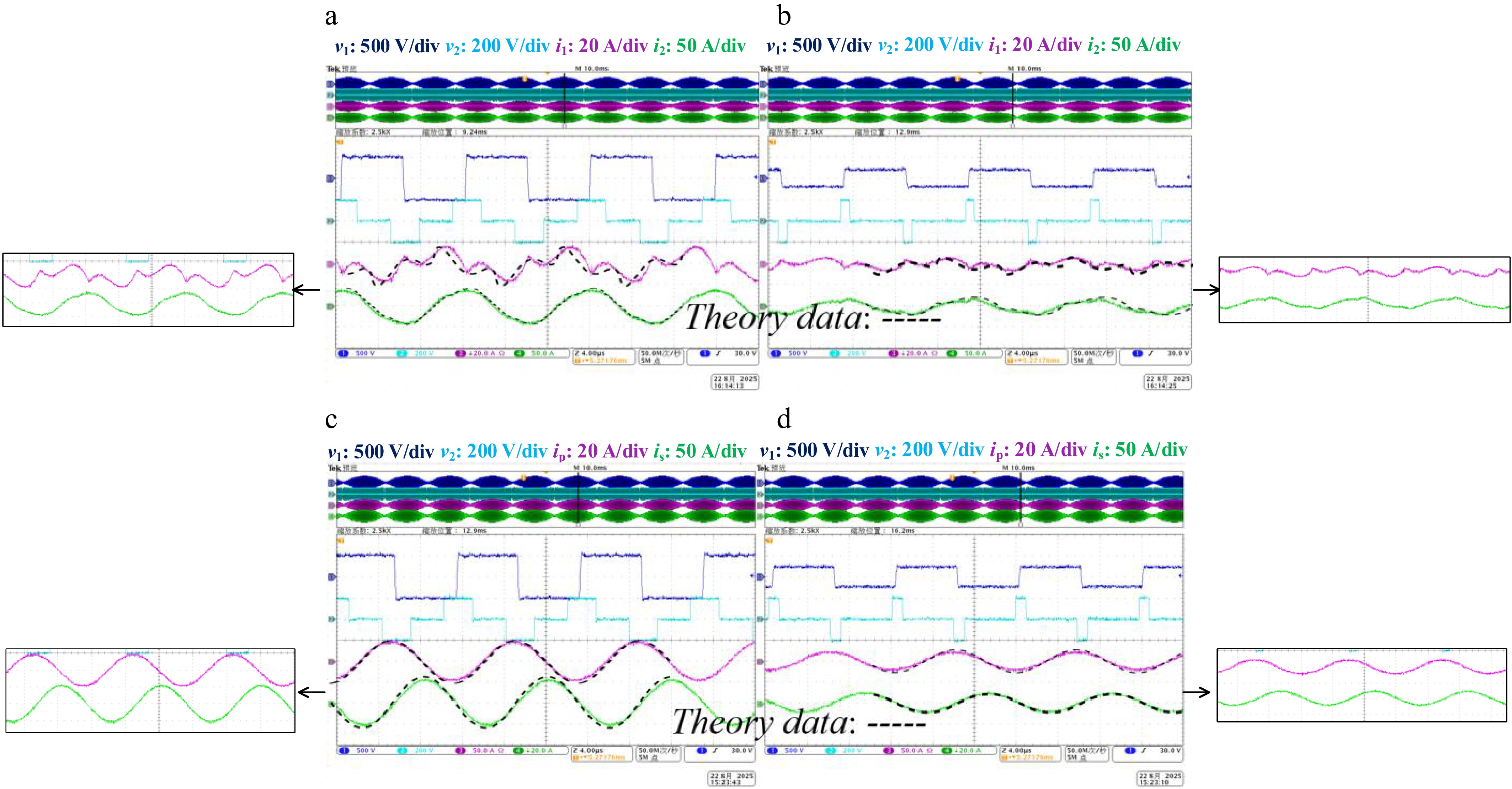
Figure 12.
Experiment validation of φ = −0.5 for V2G. (a) Maximum v_ac with i₁ and i₂. (b) Low v_ac with i₁ and i₂. (c) Steady-state waveforms with i_p and i_s. (d) Low v_ac with i_p and i_s.
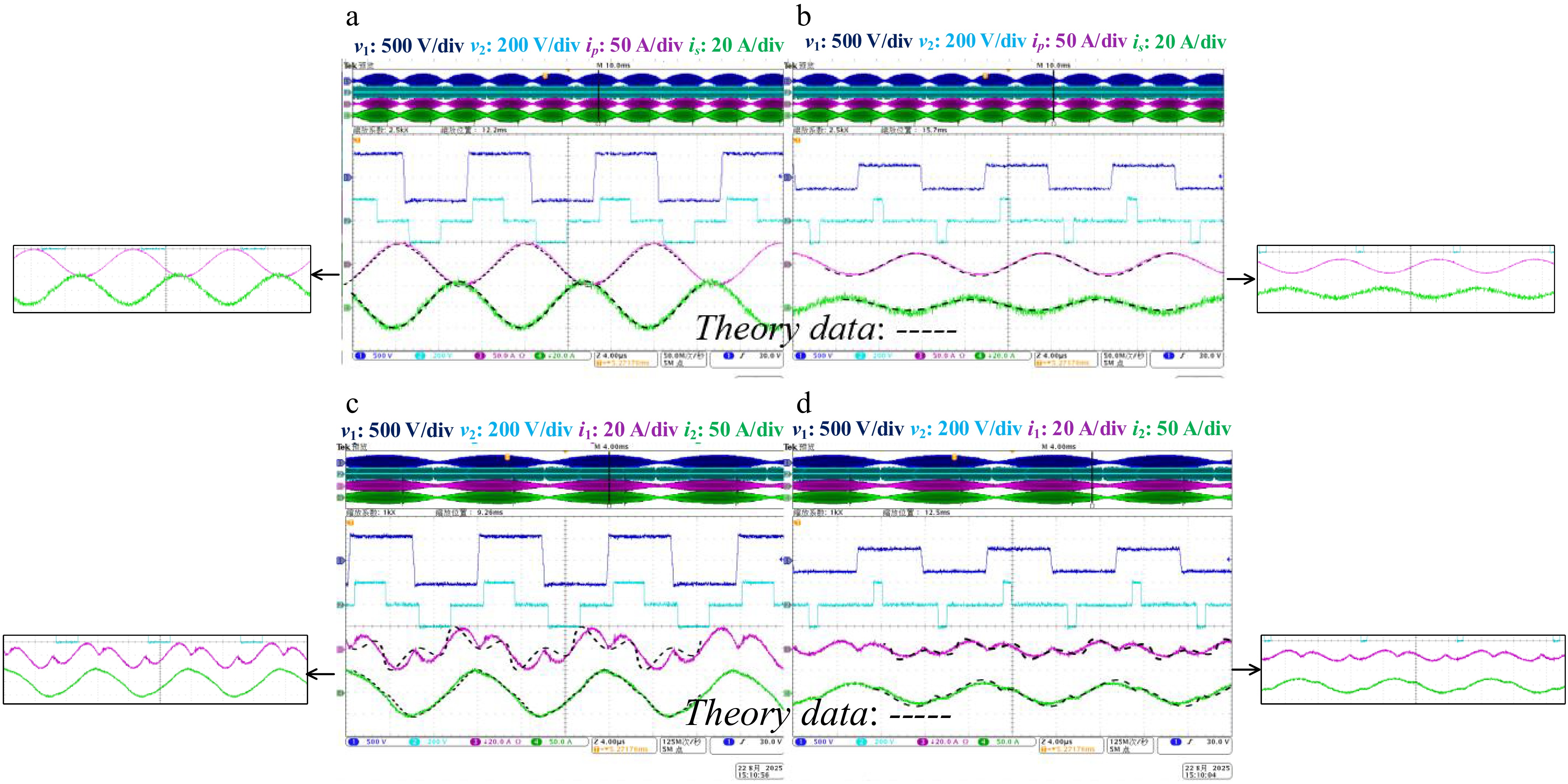
Figure 13.
Experiment validation of φ = −0.2 for V2G. (a) Maximum v_ac with i₁ and i₂. (b) Low v_ac with i₁ and i₂. (c) Maximum v_ac with i_p and i_s. (d) Low v_ac with i_p and i_s
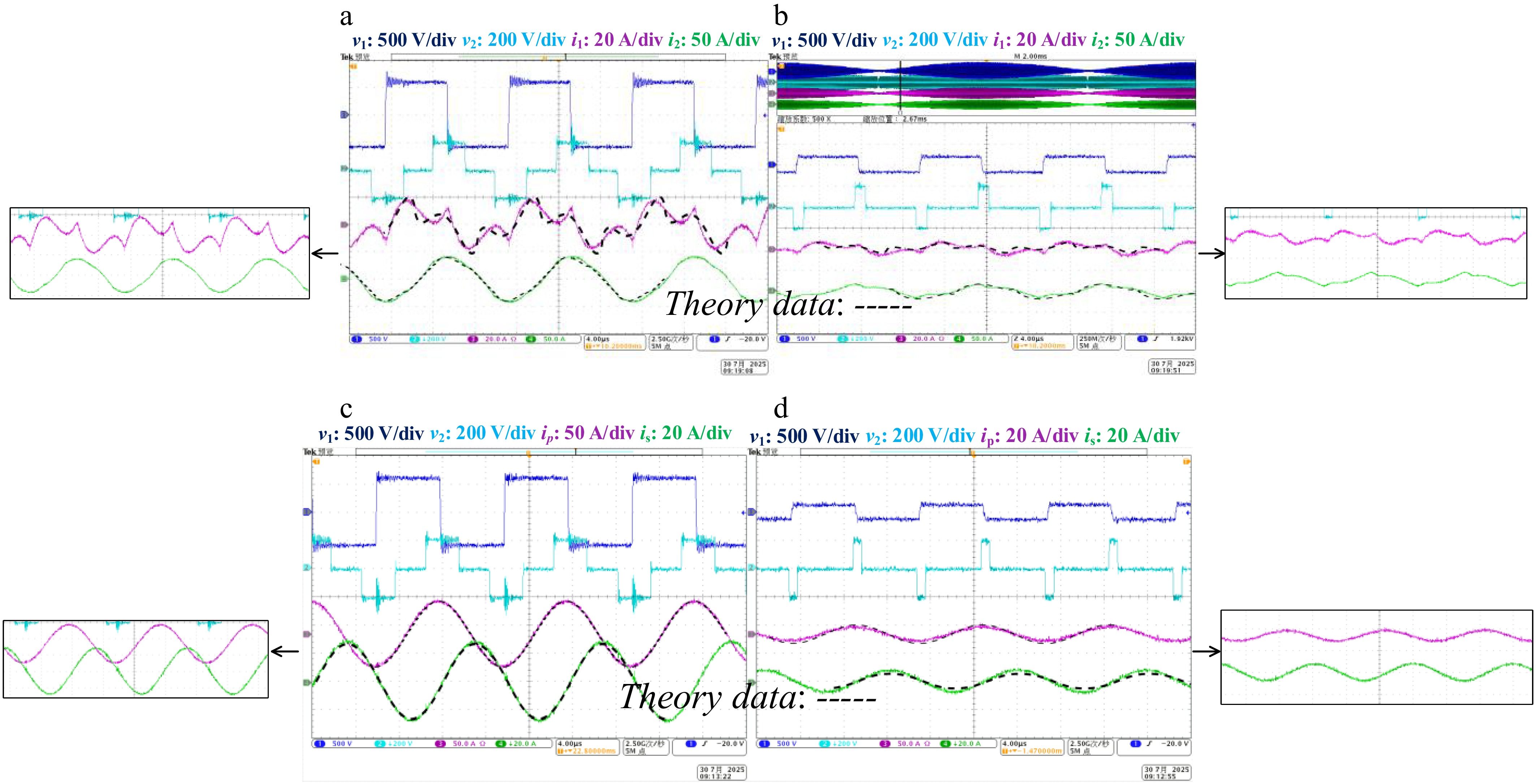
Figure 14.
Experiment validation of φ = 0.5 for G2V. (a) Maximum v_ac with i₁ and i₂. (b) Low v_ac with i₁ and i₂. (c) Maximum v_ac with i_p and i_s. (d) Low v_ac with i_p and i_s.
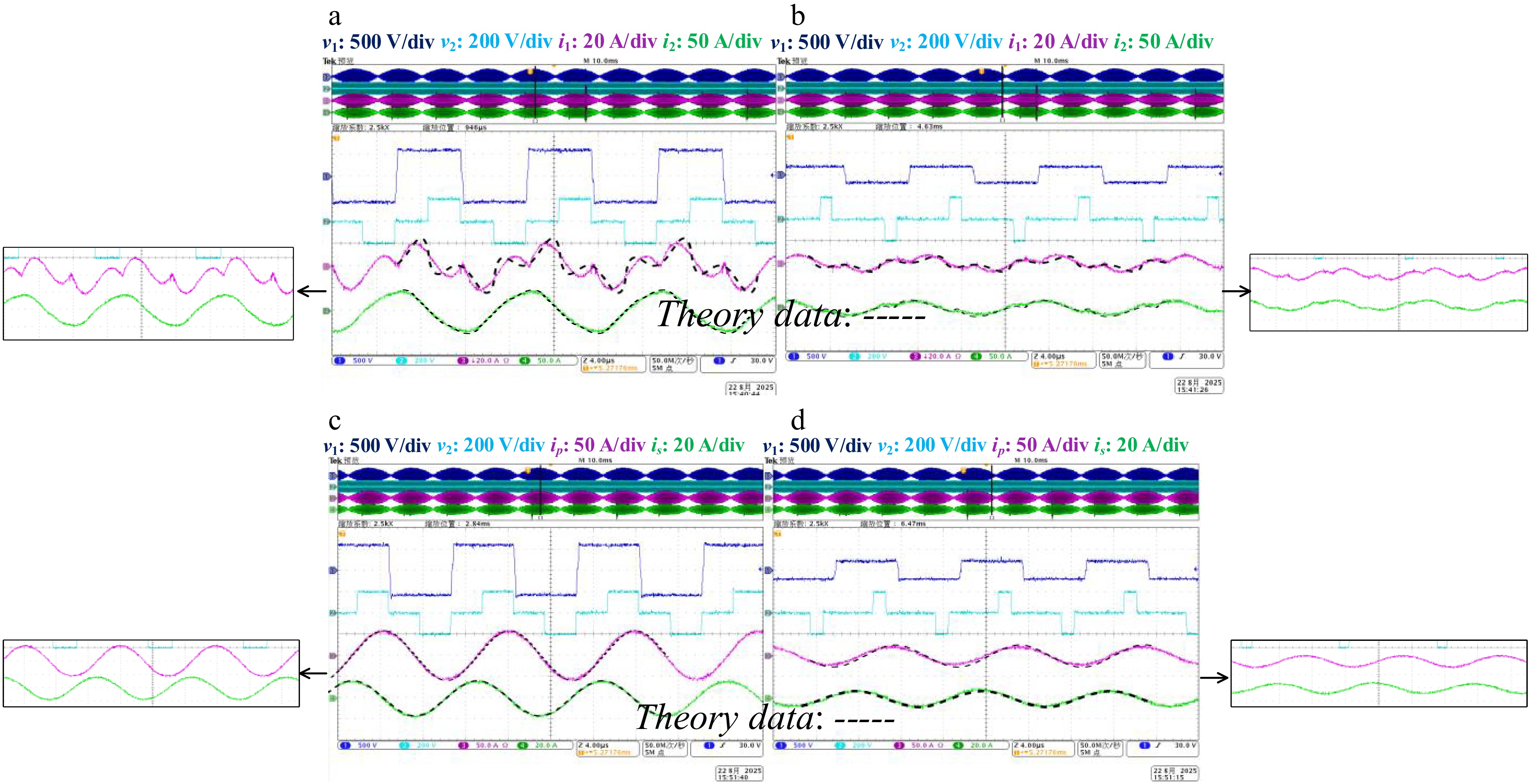
Figure 15.
Experiment validation of φ = 0.2 for G2V. (a) Maximum v_ac with i₁ and i₂. (b) Low v_ac with i₁ and i₂. (c) Maximum v_ac with i_p and i_s. (d) Low v_ac with i_p and i_s.
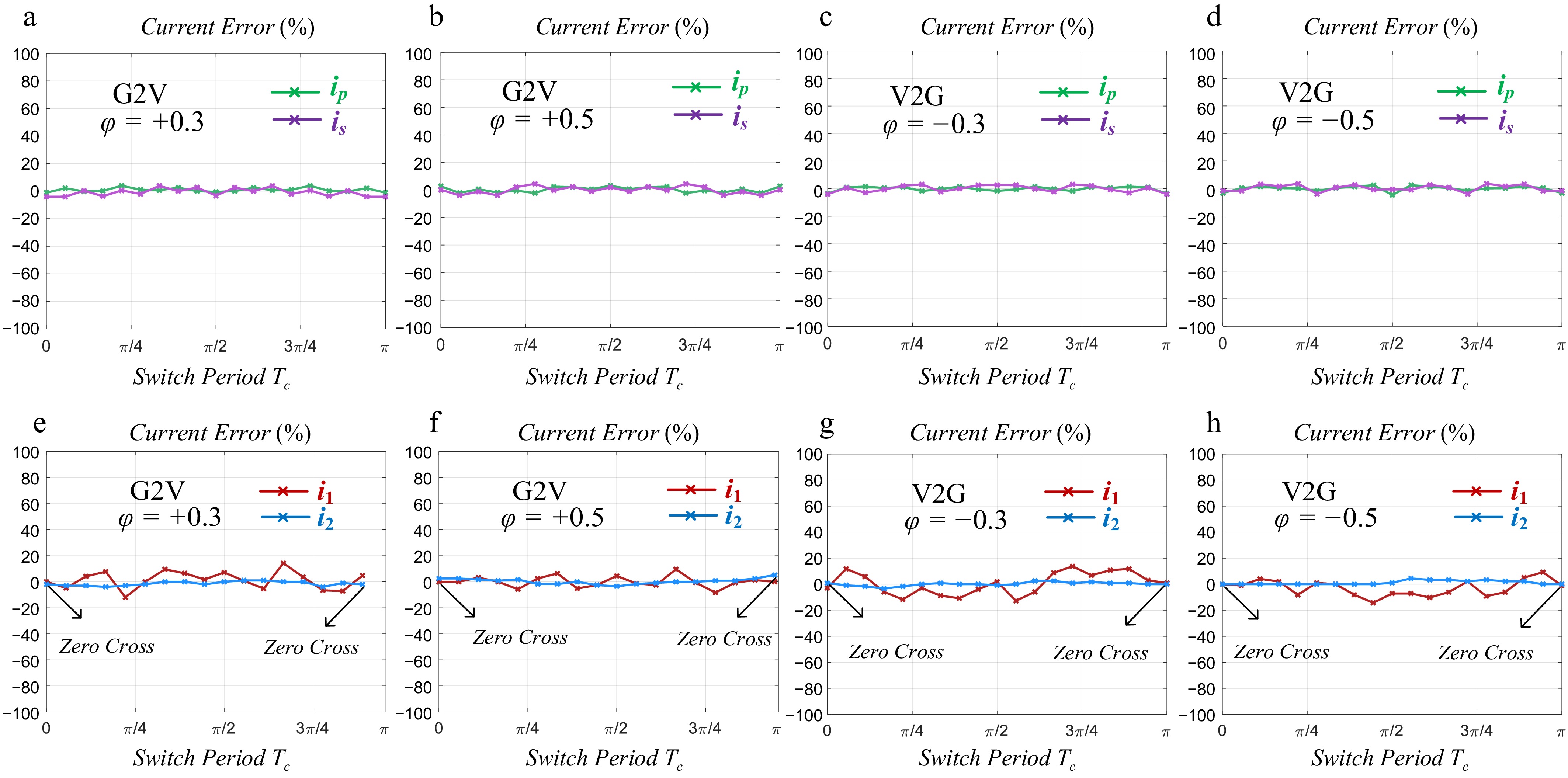
Figure 16.
The error of passive network currents under different phase shifts and different power transfer directions. (a) i_p and i_s for φ = +0.3. (b) i_p and i_s for φ = +0.5. (c) i_p and i_s for φ = −0.3. (d) i_p and i_s for φ = −0.5. (e) i₁ and i₂ for φ = +0.3. (f) i₁ and i₂ for φ = +0.5. (g) i₁ and i₂ for φ = −0.3. (h) i₁ and i₂ for φ = −0.5.
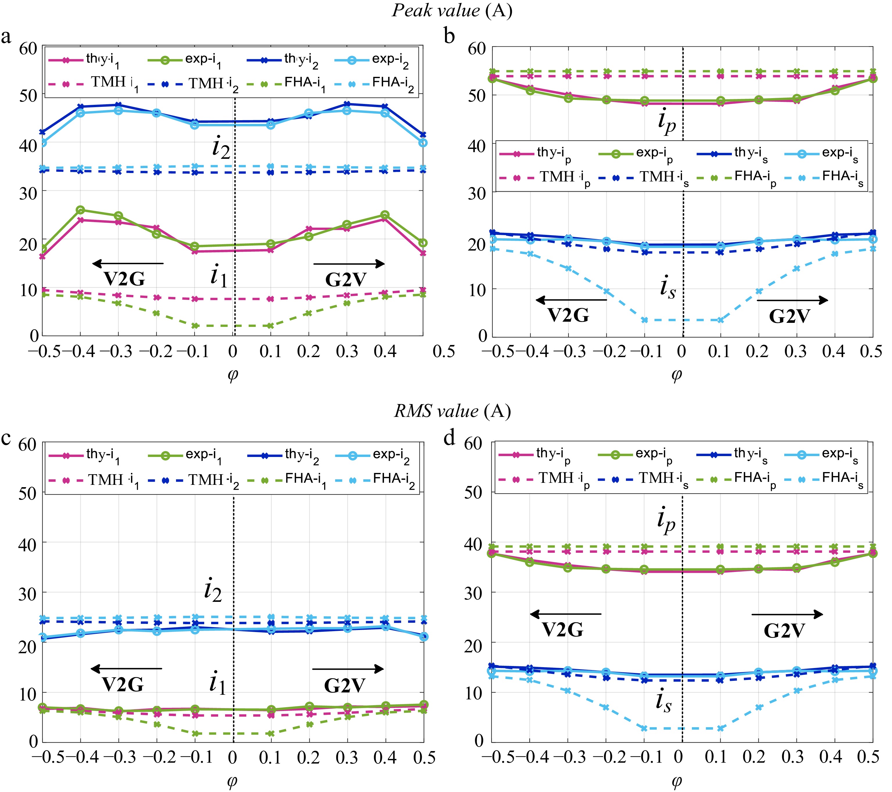
Figure 17.
Experiment validation data ('thy' for 'theory', 'exp' for 'experiment'). (a) i₁ and i₂ for amplitude. (b) i_p and i_s for amplitude. (c) i₁ and i₂ for RMS value. (d) i_p and i_s for RMS value.

Symbol	Concept	Expression
Z_L1	Transmitter side filter inductor impedance	$ {R_1} + j\omega M{L_1} $
Z_C1	Transmitter side filter capacitor impedance	$ {1 \mathord{\left/ {\vphantom {1 {j\omega {C_1}}}} \right. } {j\omega {C_1}}} $
Z_p	Transmitter side series impedance	$ {R_p} + j\omega {L_p} + {1/{j\omega {C_p}}} $
Z_s	Receiver side series impedance	$ {R_s} + j\omega {L_s} + {1 \mathord{\left/ {\vphantom {1 {j\omega {C_s}}}} \right. } {j\omega {C_s}}} $
Z_L2	Receiver side filter inductor impedance	$ {R_2} + j\omega M{L_2} $
Z_C2	Receiver side filter capacitor impedance	$ {1 \mathord{\left/ {\vphantom {1 {j\omega {C_2}}}} \right. } {j\omega {C_2}}} $

Table 1.

Expression of impedance in passive network.

Symbol	Concept	Expression
L₁/R₁	Transmitter side filter inductor impedance / internal resistance	23 μH/0.02 Ω
C₁	Transmitter side filter capacitor impedance	152.43 nF
C_p	Transmitter side series capacitor	149.19 nF
L_p/R_p	Transmitter side series inductor / internal resistance	46.49 μH/0.02 Ω
L₂/R₂	Receiver side filter inductor impedance / internal resistance	14 μH/0.02 Ω
C₂	Receiver side filter capacitor impedance	250.42 nF
C_s	Receiver side series capacitor	246.55 nF
L_s/R_s	Receiver side series inductor / internal resistance	29.73 μH/0.02 Ω
f_c	Resonant frequency	85 kHz
f_l	Grid frequency	50 Hz
M	Mutual Inductor	10.04 μH

Table 2.

Example parameters of BWPT system.

Method type	Peak value (A)				RMS value (A)				Mean value of current error
Method type	i₁	i₂	i_p	i_s	i₁	i₂	i_p	i_s	i₁	i₂	i_p	i_s
FHA	9.1	34.8	55.8	17.6	7.6	25.1	39.8	13.3	/	/	/	/
TMH	9.8	34.4	55.5	20.9	8.2	24.6	38.5	15.6	/	/	/	/
thy(FTDC)	17.7	42.0	55.3	20.9	8.3	20.6	38.4	15.5	7.8%	2.1%	1.2%	1.9%
exp(Experiment)	19.6	39.9	55.3	20.0	8.3	20.6	38.4	14.7	7.8%	2.1%	1.2%	1.9%

Table 3.

Detailed data of FTDC calculation and experiment with φ = +0.5.

Method type	Peak value (A)				RMS value (A)				Mean value of current error
Method type	i₁	i₂	i_p	i_s	i₁	i₂	i_p	i_s	i₁	i₂	i_p	i_s
FHA	4.8	35	55.8	14.2	5.8	24.9	39.8	10.2	/	/	/	/
TMH	9.2	34.7	54.9	19.3	6.2	23.6	37.9	13.6	/	/	/	/
thy(FTDC)	23.3	47.9	50.0	20.3	6.3	22.8	35.5	14.8	12.2%	2.3%	1.7%	1.8%
exp(Experiment)	24.8	46.1	49.7	20.2	6.2	22.8	35.3	14.7	12.2%	2.3%	1.7%	1.8%

Table 4.

Detailed data of FTDC calculation and experiment with φ = −0.3.

Method type	Amount of calculation	Number of order n	BWPT support	Computational complexity	Compensation network	Three feature outputs	Accuracy (for feature outputs)
FHA	Small	1	Yes	Simple	Unrestricted	Average only	Low
GSSA	Large	Infinite	Yes	Very complex	Unrestricted	Average only	High
TMH analysis^[18−20]	Medium	Not mentioned	No	Medium	Unrestricted	All	Medium
Sample-data model^[21]	Large	Infinite	No	Complex	SS	Average only	Very high
harmonics-considered time-domain model^[22]	Small	Not mentioned	No	Medium	Unrestricted	All	Medium
Discrete-time model^[23]	Very large	9	No	Complex	DLCC	All	Very high
Proposed FTDC	Medium	3, 9	Yes	Medium	Unrestricted	All	High

Table 5.

Comparison between various methods in WPT application.