


-
Bidirectional Wireless Power Transfer (BWPT) systems are essential in the context of electric vehicles (EVs), enabling the efficient bidirectional power exchange between the Grid and Vehicle (G2V), and Vehicle to Grid (V2G) operations[1−4].
In BWPT systems, the traditional two-stage converter structure at the transmitter suffers from drawbacks such as large volume, high cost, and complex control[1]. Consequently, replacing the conventional two-stage structure with a single-stage AC-AC converter at the transmitter has become a current research trend in BWPT systems. Among single-stage AC-AC converters, the matrix converter eliminates the large-capacitance DC bus capacitor but still requires eight high-frequency switches[5−8]. Moreover, it faces issues such as low voltage gain, significant dead-time effects, and limited soft-switching capability. The buck–boost type single-stage AC-AC converter reduces the number of switches compared to the matrix converter[9−12], but it does not resolve the soft-switching limitations. The Bridgeless Full Bridge (BFB) converter halves the number of switches and offers advantages such as high voltage gain and a wide soft-switching range[13]; however, it retains large electrolytic capacitors, and its control system is still highly complex.
In contrast, the single-stage totem-pole converter strikes a compromise, eliminating the drawbacks of the above topologies while combining the benefits of fewer switches, a small DC bus capacitor, and high voltage gain[14]. Furthermore, with Triple Phase Ratio Shift (TPRS) control, it not only achieves power factor correction (PFC) but also further expands the soft-switching range of the system[15]. Nevertheless, current research on BWPT systems employing totem-pole converters, as presented in this paper, remains limited; the modeling and analysis of such systems is critical for optimizing their performance and ensuring reliable power transmission.
A range of approaches has been proposed for the circuit analysis of BWPT systems, each serving specific purposes. In passive network analysis, a spatial state model is introduced that represents the parameters of passive networks[16], along with voltage and current, in matrix form. This representation simplifies the calculation process, albeit at the expense of model realism and detail. Another study[17] proposed a steady-state model for BWPT systems, focusing on the effects of battery voltage fluctuations in EVs under varying load conditions. Both these methods rely on the FHA, which simplifies the voltage transformation in the converter by considering only the effective value in the fundamental state, thereby neglecting the time-domain dynamics of the system.
Beyond the FHA method, researchers have explored alternative ways to analyze BWPT systems. Notably, the harmonics current method[18,19] that decomposes the current in passive networks, treating each harmonic component as an independent passive network. This approach, while offering reasonable accuracy, requires additional components such as filters, which can increase the system's size and losses. The multi-harmonics analysis method[20] offers a more comprehensive approach by decomposing complex voltage and current waveforms into their harmonic components in the frequency domain. It analyzes higher-order harmonics and reconstructs the waveforms to approximate the actual voltage and current values. However, this method has a significant drawback: its inability to integrate with the time domain limits its effectiveness, particularly in capturing the phase differences between the primary and secondary voltages in bidirectional systems.
These methods are collectively referred to as Traditional Multi-harmonics (TMH) techniques, which, while accurate in the frequency domain, lack phase correction in time-domain processing. This is particularly problematic in BWPT systems based on single-stage AC-AC converters, where both the amplitude and phase of voltage and current in the passive network continuously fluctuate due to grid voltage variations. As a result, accurately modeling these systems under such complex operating conditions remains a significant challenge when using TMH methods.
To address the limitations of TMH methods, several researchers have suggested time-domain-based approaches. The sampled-data modeling method[21] is proposed for analyzing the system parameters of BWPT, ensuring accuracy through time-domain calculations. However, this method is limited to sinusoidal current analysis and does not apply to non-sinusoidal currents in Double LCC (DLCC) systems. Other studies[22,23] introduced discrete time-domain models that decompose and synthesize current solutions over different time intervals to reconstruct waveforms. However, these models are restricted to networks with a single voltage source. When additional complexities, such as active rectifiers on the secondary side and phase shifts between the primary and secondary sides, are introduced, the models become significantly more complicated. This often results in complex mathematical derivations that are difficult to apply under dynamic BWPT operating conditions. Furthermore, despite considering all possible scenarios, these approaches struggle to provide convergent solutions, leading many researchers to rely more on simulation tools than theoretical models.
In this context, this paper proposes a novel Frequency-Time Domain Combined (FTDC) analysis prediction method for BWPT systems[24]. This method employs a single-stage totem-pole AC-AC converter to integrate both time-domain and frequency-domain analyses. The approach provides accurate square wave voltages, precise sine currents, and relatively accurate non-sinusoidal currents in passive networks. By extracting key parameters such as amplitude, phase, effective value, and zero-crossing points, this method enables more accurate predictions of actual system behavior.
The paper proceeds by first establishing the theoretical framework for the BWPT high-order harmonics model. It then derives the system characteristic variables using the combined frequency and time-domain methods, producing theoretical predictions. To validate these findings, an experimental platform is developed, and the collected data is analyzed to assess the accuracy and practical applicability of the proposed FTDC method.
This paper begins by establishing and deriving the BWPT high-order harmonics model through theoretical analysis. It then derives the system characteristic variables using a combination of frequency and time-domain methods, resulting in theoretical predictions. An experimental platform was subsequently set up to validate the accuracy of these theoretical findings. Finally, the collected data were organized and analyzed to evaluate both the accuracy and practical applicability of the proposed FTDC analysis method.
-
Figure 1a illustrates the schematic circuit of the BWPT system, which is based on a single-stage AC-AC converter utilized in this paper. The primary converter is designed with a single-stage totem pole structure, while the secondary converter employs an active rectifier. The compensation network is configured using a DLCC structure. Figure 1b presents the equivalent circuit, and the expressions for each passive impedance are detailed in Table 1.
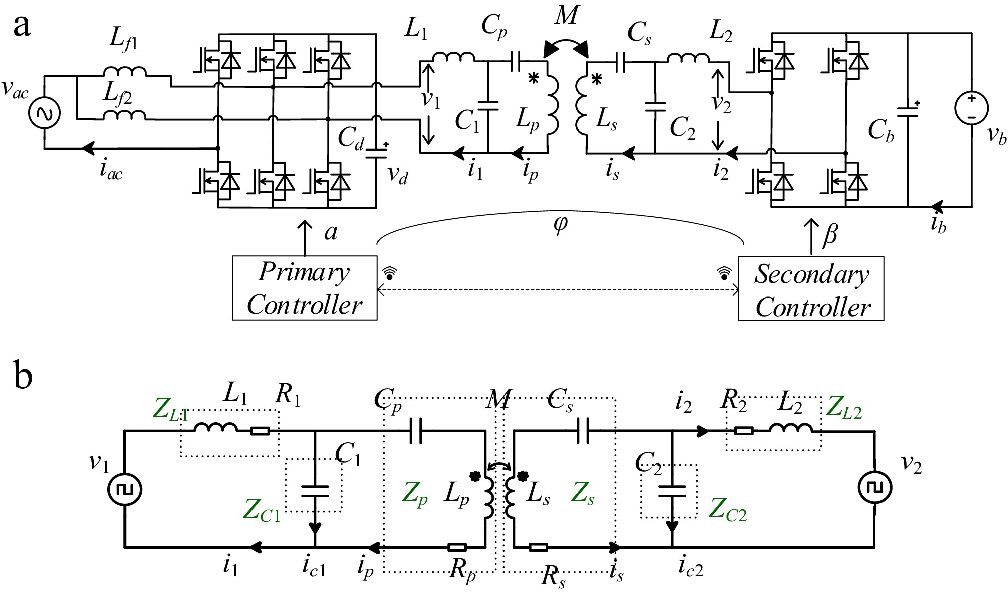
Figure 1.
Schematic of BWPT system. (a) BWPT circuit with totem converter. (b) Equivalent circuit with linear elements.
Table 1. Expression of impedance in passive network.
Symbol Concept Expression ZL1 Transmitter side filter inductor impedance $ {R_1} + j\omega M{L_1} $ ZC1 Transmitter side filter capacitor impedance $ {1 \mathord{\left/ {\vphantom {1 {j\omega {C_1}}}} \right. } {j\omega {C_1}}} $ Zp Transmitter side series impedance $ {R_p} + j\omega {L_p} + {1/{j\omega {C_p}}} $ Zs Receiver side series impedance $ {R_s} + j\omega {L_s} + {1 \mathord{\left/ {\vphantom {1 {j\omega {C_s}}}} \right. } {j\omega {C_s}}} $ ZL2 Receiver side filter inductor impedance $ {R_2} + j\omega M{L_2} $ ZC2 Receiver side filter capacitor impedance $ {1 \mathord{\left/ {\vphantom {1 {j\omega {C_2}}}} \right. } {j\omega {C_2}}} $ Figure 2a depicts the schematic diagram of the AC side voltage at the primary and secondary sides. This paper adopts a three-shift-ratio control mode, wherein the target control parameters are achieved by adjusting the internal phase shift of the primary side totem-pole converter (or called totem converter), the internal phase shift ratio of the secondary side active bridge, and the external shift ratio comparison between the primary and secondary side converters.
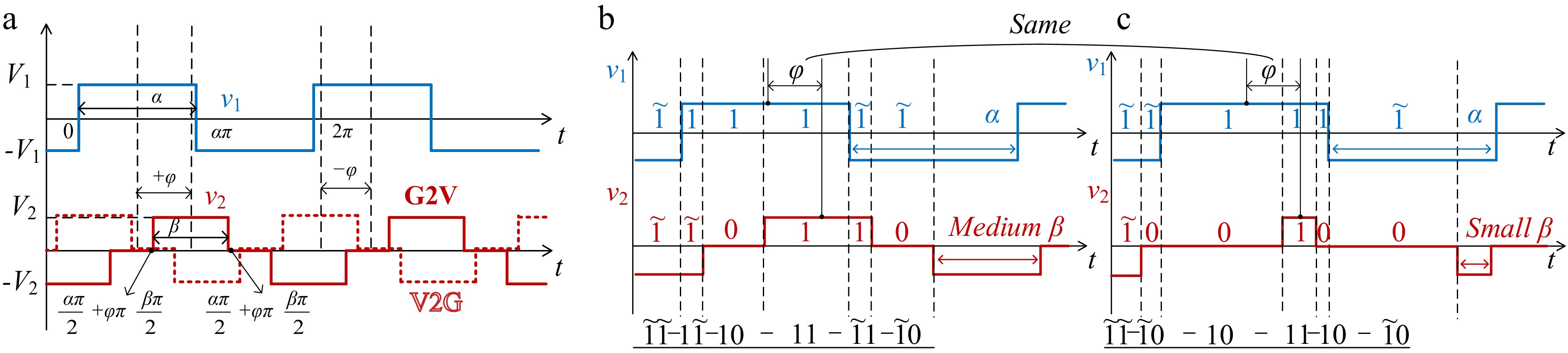
Figure 2.
Schematic of transmitter and receiver side voltage phase shift. (a) Bidirectional voltage phase delay schematic. (b) Medium β for the system. (c) Small β for the system.
Figure 2b, c explains why a time-domain only analysis method can't derive an accurate model for the single-stage BWPT system possessing phase shift delay. When β changes from medium to small, the voltage sequence between the primary side and the secondary side changes, resulting in the established model being completely rebuilt from scratch. Not to mention, the time-varying nature of the phase shift will also lead to inaccuracies in the frequency-domain TMH method due to the constantly changing phase difference.
In conclusion, they fail to capture various critical details during transient conditions. This includes the amplitudes of voltage and current, the soft switching states of the converter, and other dynamic behaviors.
To address these limitations and enable rapid predictions of the system's working state without reliance on simulation or experimental platforms, this paper proposes an FTDC method that balances between the frequency domain and time domain analysis.
First, the harmonics frequency AC side voltages v1 and v2 of the primary and secondary side can be expressed as:
$ \mathop {{v_{1,n}}(t)}\limits_{n = 1,3,5 \cdots } = \dfrac{4}{\pi }{V_d}\dfrac{1}{n}\cos \left( {n\omega t - \dfrac{{n\alpha }}{2}} \right)\sin \left( {\dfrac{{n\alpha }}{2}} \right) $ (1) $ \mathop {{v_{2,n}}(t)}\limits_{n = 1,3,5 \cdots } = \dfrac{4}{\pi }{V_b}\dfrac{1}{n}\cos \left( {n\omega t - \dfrac{{n\alpha }}{2} + n\varphi } \right)\sin \left( {\dfrac{\beta }{2}\pi } \right) $ (2) where, ɑ, β, and φ are three shift ratios of the primary and secondary side voltages. Vd and Vb are the steady values of the DC bus voltage of the primary and secondary converter of vd and vb, respectively. n is the order of harmonics. ω is the working frequency of the system, and the system generally works at the resonant frequency ωc.
$ {\omega _c} = \dfrac{1}{{\sqrt {{L_1}{C_1}} }} = \dfrac{1}{{\sqrt {{L_2}{C_2}} }} $ (3) $ {\omega _c} = \dfrac{1}{{\sqrt {\dfrac{{{L_p}\left( {{C_1} + {C_p}} \right)}}{{{C_1}{C_p}}}} }} = \dfrac{1}{{\sqrt {\dfrac{{{L_s}\left( {{C_2} + {C_s}} \right)}}{{{C_2}{C_s}}}} }} $ (4) FTDC analysis aims to theoretically represent the voltage and current waveforms of passive networks. According to Eqs (1) and (2), when employing the FHA method, only the fundamental voltage component is typically selected as the primary factor for calculations. However, it is essential to consider the higher-order harmonics of the voltage and current. The independent variable matrix x of the passive network can be expressed as:
$ {\boldsymbol{x}} = {\left[ {\begin{array}{*{20}{c}} {{v_{1,1}}}&{{i_{1,1}}}&{{i_{p,1}}}&{{i_{s,1}}}&{{i_{2,1}}}&{{v_{2,1}}} \\ {{v_{1,3}}}&{{i_{1,3}}}&{{i_{p,3}}}&{{i_{s,3}}}&{{i_{2,3}}}&{{v_{2,3}}} \\ \vdots & \vdots & \vdots & \vdots & \vdots & \vdots \\ {{v_{1,n}}}&{{i_{1,n}}}&{{i_{p,n}}}&{{i_{s,n}}}&{{i_{2,n}}}&{{v_{2,n}}} \end{array}} \right]^T} $ (5) According to the KCL and KVL equations, the nth harmonics coefficient matrix An can be expressed as:
$ {{\boldsymbol{A}}_n} = \left[ {\begin{array}{*{20}{c}} 1&{ - \left( {{Z_{L1,n}} + {Z_{C1,n}}} \right)}&{{Z_{C1,n}}}&0&0&0 \\ 1&{ - {Z_{L1,n}}}&{ - {Z_{p,n}}}&{jn\omega M}&0&0 \\ 0&0&{jn\omega M}&{ - {Z_{s,n}}}&{ - {Z_{L2,n}}}&{ - 1} \\ 0&0&0&{{Z_{C2,n}}}&{ - \left( {{Z_{L2,n}} + {Z_{C2,n}}} \right)}&{ - 1} \end{array}} \right] $ (6) $ {\boldsymbol{A}} = diag\left\{ {{{\boldsymbol{A}}_1},{{\boldsymbol{A}}_3},{{\boldsymbol{A}}_5}, \cdots {{\boldsymbol{A}}_n}} \right\} $ (7) $ {\boldsymbol{Ax}} = {{\boldsymbol{O}}_{4n \times n}} $ (8) If the square wave voltage is decomposed into its constituent sinusoidal high-order harmonics currents using the homogeneous theorem, the aforementioned frequency domain calculation method can be effectively applied during each complete cycle of operation. This approach allows for a more accurate representation of the system's behavior by considering the contributions of each harmonics component to the overall waveform, facilitating better analysis and design of passive networks.
Based on the homogeneous theorem, the voltage and current within the passive network can be decomposed into various harmonic components. With a specific number of harmonics considered, the passive impedance network will exhibit relevant characteristics at those corresponding frequencies. Each individual circuit can be analyzed in the frequency domain to satisfy the relationships defined by the state equations. This approach allows for the derivation of a new state equation that reflects the behavior of the network under the influence of these harmonics. Figure 3 is a schematic diagram of the phase of voltage and current in a passive network within a BWPT system. Taking G2V as an example, v1 leading i1 ensures one of the basic conditions for ZVS of the primary side converter. Regardless of how the phase shift φ changes, ip and v1, as well as is and v2, always maintain an almost π/2 phase difference.
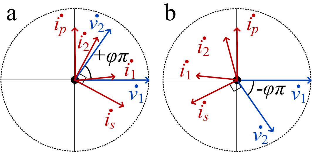
Figure 3.
Schematic diagram of voltage and current phases in a passive network. (a) G2V. (b) V2G.
Further derivation of Eq. (2) using the Trigonometric function[25]
$ {v_{2,n}}\left( t \right) = \dfrac{4}{\pi }{V_b}\dfrac{1}{n}\left( \begin{gathered} \cos \left( {n\omega t - \dfrac{{n\alpha }}{2}} \right)\cos \left( {n\varphi } \right) \\ - j\cos \left( {n\omega t - \dfrac{{n\alpha }}{2}} \right)\sin \left( {n\varphi } \right) \\ \end{gathered} \right)\sin \left( {\dfrac{{n\beta }}{2}} \right) $ (9) We can get
$ {v_{2,n}}\left( t \right) = \dfrac{4}{\pi }\left( {\cos \left( \varphi \right) + j\sin \left( \varphi \right)} \right)\cos \left( {n{\omega _s}t - \dfrac{{\alpha \pi }}{2}} \right)\sin \left( {\dfrac{{\beta \pi }}{2}} \right){V_b} $ (10) Through derivation, the secondary side current i2 can be expressed as:
$ {i_{2,n}} = \dfrac{{{Z_{C1,n}}}}{{{\Psi _{2,n}}}}{v_{1,n}} + \dfrac{{{\Psi _{1,n}}}}{{{\Psi _{2,n}}}}{v_{2,n}} $ (11) where,
$ \begin{gathered} {\Psi _{1,n}} = \dfrac{{jn\omega M}}{{{Z_{C2,n}}}}\left( {{Z_{L1,n}} + {Z_{C1,n}}} \right) - \\ \dfrac{1}{{jn\omega M}}\left( {{Z_{p,n}}\left( {{Z_{L1,n}} + {Z_{C1,n}}} \right) + {Z_{C1,n}}{Z_{L1,n}}} \right)\left( {\dfrac{{{Z_{s,n}}}}{{{Z_{C2,n}}}} + 1} \right) \\ \end{gathered} $ (12) $ \begin{split} {\Psi _{2(n)}} =\;& \dfrac{1}{{jn\omega M}}\left( {{Z_{p,n}}\left( {{Z_{L1,n}} + {Z_{C1,n}}} \right) + {Z_{C1,n}}{Z_{L1,n}}} \right)\left( \begin{gathered} \dfrac{{{Z_{L2,n}}}}{{{Z_{C2,n}}}}{Z_{s,n}} \\ + {Z_{s.n}} + {Z_{L2,n}} \\ \end{gathered} \right) \\& - jn\omega M\left( {\dfrac{{{Z_{L2,n}}}}{{{Z_{C2,n}}}} + 1} \right)\left( {{Z_{L1,n}} + {Z_{C1,n}}} \right) \\ \end{split} $ (13) $ {{\boldsymbol{\Psi }}_1} = diag\left\{ {{\Psi _{1,1}},{\Psi _{1,3}},{\Psi _{1,5}}, \cdots {\Psi _{1,n}}} \right\} $ (14) $ {{\boldsymbol{\Psi }}_2} = diag\left\{ {{\Psi _{2,1}},{\Psi _{2,3}},{\Psi _{2,5}}, \cdots {\Psi _{2,n}}} \right\} $ (15) The time-domain representation of matrix i2, which includes multiple harmonics, is as follows:
$ {{\boldsymbol{i}}_2}\left( t \right) = {{\boldsymbol{x}}_{:,5}}\left( t \right) = \left( {{{\boldsymbol{Z}}_{C1}}{{\boldsymbol{v}}_1}\left( t \right) + {{\boldsymbol{\Psi }}_1}{{\boldsymbol{v}}_2}\left( t \right)} \right){\boldsymbol{\Psi }}_{_2}^{ - 1} $ (16) $ {{\boldsymbol{i}}_2}\left( t \right) = {{\boldsymbol{x}}_{:,5}}\left( t \right) = {{\boldsymbol{Y}}_{21}}{{\boldsymbol{v}}_1}\left( t \right) + {{\boldsymbol{Y}}_{22}}{{\boldsymbol{v}}_2}\left( t \right) $ (17) where, Y21 and Y22 are the coefficient admittance matrix, corresponding to v1 and v2 respectively. Based on i2(n), other current expressions ip, i1, is in passive networks can be derived
$ {i_{p,n}} = \dfrac{1}{{jn\omega M}}\left( {\dfrac{{{i_{2,n}}{Z_{L2,n}} + {v_{2,n}}}}{{{Z_{C2,n}}}}{Z_{s,n}} + {i_{2,n}}({Z_{s,n}} + {Z_{L2,n}}) + {v_{2,n}}} \right) $ (18) $ {{\boldsymbol{i}}_p} = \left[ {\begin{array}{*{20}{c}} {{i_{p,1}}}&{{i_{p,3}}}& \cdots &{{i_{p,n}}} \end{array}} \right] $ (19) $ {{\boldsymbol{i}}_p}\left( t \right) = {{\boldsymbol{x}}_{:,3}}\left( t \right) = {{\boldsymbol{Y}}_{p1}}{{\boldsymbol{v}}_1}\left( t \right) + {{\boldsymbol{Y}}_{p2}}{{\boldsymbol{v}}_2}\left( t \right) $ (20) $ {i_{1,n}} = \dfrac{{{v_1}_{,n} + {i_{p,n}}{Z_{C1,n}}}}{{{Z_{L1,n}} + {Z_{C1,n}}}} $ (21) $ {{\boldsymbol{i}}_1} = \left[ {\begin{array}{*{20}{c}} {{i_{1,1}}}&{{i_{1,3}}}& \cdots &{{i_{1,n}}} \end{array}} \right] $ (22) $ {{\boldsymbol{i}}_1}\left( t \right) = {{\boldsymbol{x}}_{:,1}}\left( t \right) = {{\boldsymbol{Y}}_{11}}{{\boldsymbol{v}}_1}\left( t \right) + {{\boldsymbol{Y}}_{12}}{{\boldsymbol{v}}_2}\left( t \right) $ (23) $ {i_{s,n}} = \dfrac{{{i_{2,n}}{Z_{L2,n}} + {v_{2,n}}}}{{{Z_{C2,n}}}} + {i_{2,n}} $ (24) $ {{\boldsymbol{i}}_s} = \left[ {\begin{array}{*{20}{c}} {{i_{s,1}}}&{{i_{s,3}}}& \cdots &{{i_{s,n}}} \end{array}} \right] $ (25) $ {{\boldsymbol{i}}_s}\left( t \right) = {{\boldsymbol{x}}_{:,4}}\left( t \right) = {{\boldsymbol{Y}}_{s1}}{{\boldsymbol{v}}_1}\left( t \right) + {{\boldsymbol{Y}}_{s2}}{{\boldsymbol{v}}_2}\left( t \right) $ (26) where, Yp1 and Yp2, Y11 and Y12, Ys1 and Ys2, are the coefficient matrix corresponding to each current. The parameters of the BWPT system presented in this paper are detailed in Table 2. Figure 4a−d shows the amplitude-phase characteristic diagrams of the coefficient admittance matrix. At the fundamental frequency, which corresponds to the resonant frequency, i2 and is are independent of v1 and exhibit a high correlation with v2. Similarly, i1 and ip are independent of v1 and show a high correlation with v2. As the frequency increases to the 3rd, 5th, and higher harmonics, the amplitude attenuates, while the phase remains constant and exhibits a canceling effect.
Table 2. Example parameters of BWPT system.
Symbol Concept Expression L1/R1 Transmitter side filter inductor impedance / internal resistance 23 μH/0.02 Ω C1 Transmitter side filter capacitor impedance 152.43 nF Cp Transmitter side series capacitor 149.19 nF Lp/Rp Transmitter side series inductor / internal resistance 46.49 μH/0.02 Ω L2/R2 Receiver side filter inductor impedance / internal resistance 14 μH/0.02 Ω C2 Receiver side filter capacitor impedance 250.42 nF Cs Receiver side series capacitor 246.55 nF Ls/Rs Receiver side series inductor / internal resistance 29.73 μH/0.02 Ω fc Resonant frequency 85 kHz fl Grid frequency 50 Hz M Mutual Inductor 10.04 μH 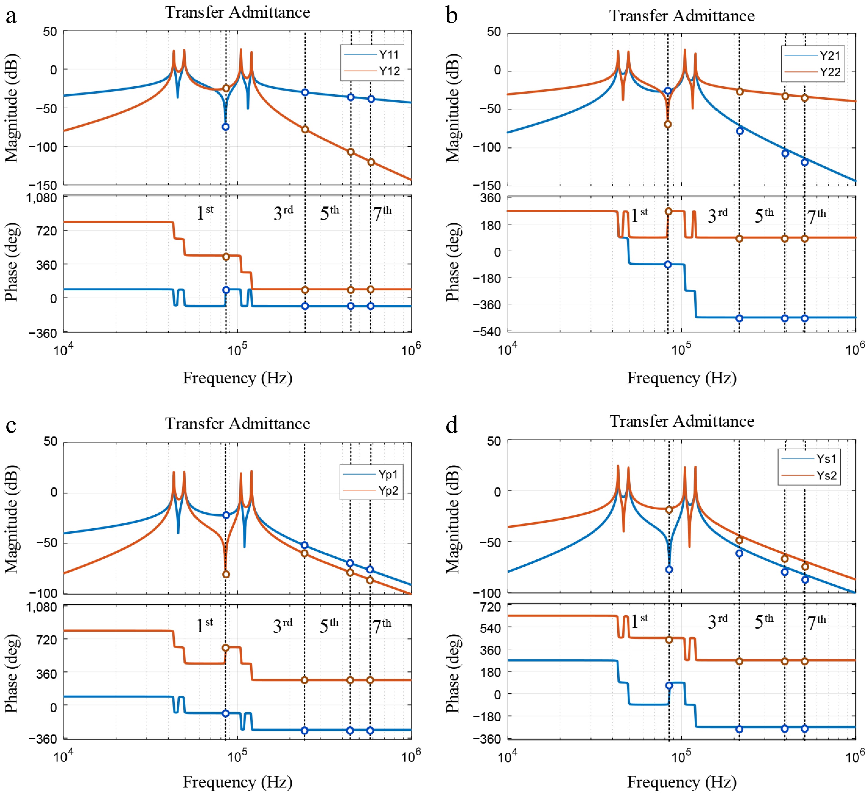
Figure 4.
Coefficient admittance matrix amplitude-phase characteristic diagram. (a) Y11 and Y12. (b) Y21 and Y22. (c) Yp1 and Yp2. (d) Ys1 and Ys2.
Figure 5 shows the FFT analysis of the currents in the passive network. It can be observed that the component of the receiving current i2 is less than 6% after the 3rd harmonic, thus higher-order harmonics can be ignored. Similarly, for the transmitting current i1, the component after the 7th harmonic is also below 5%, making further harmonics negligible. Based on this, the harmonic order for superposition is set to 7.
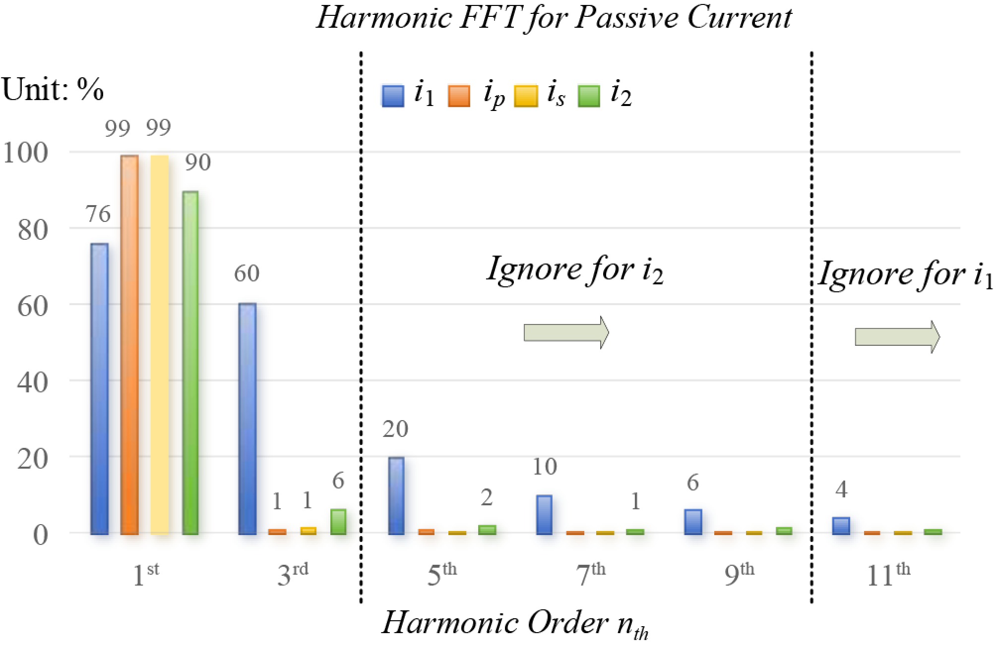
Figure 5.
Schematic diagram of the harmonics composition of each current.
$ {\hat i_{1\_\varpi }}\left( t \right) = \sum\limits_{j = 1}^n {{i_{1,j}}\left( t \right)} ,\; {\hat i_{p\_\varpi }}\left( t \right) = \sum\limits_{j = 1}^n {{i_{p,j}}\left( t \right)} ,\; n \in {\mathbb{Z}^ + } $ (27) $ {\hat i_{s\_\varpi }}\left( t \right) = \sum\limits_{j = 1}^n {{i_{s,j}}\left( t \right)} ,\; {\hat i_{2\_\varpi }}\left( t \right) = \sum\limits_{j = 1}^n {{i_{2,j}}\left( t \right)} ,\; n \in {\mathbb{Z}^ + } $ (28) The summation of the previous harmonics components is merely an expression in the frequency domain; the time domain and phase shift components need to be added. Voltage phase correction ratio φv1_nth、φv2_nth can be expressed as:
$ {\varphi _{v1\_nth}} = \dfrac{{\left( {n - 1} \right)\alpha \pi }}{2} ,\; {\varphi _{v2\_nth}} = \left( {n - 1} \right)\pi \left( {\dfrac{\alpha }{2} + \varphi } \right) $ (29) where, n equals to 1, 3, 5, 7, ···, based on the phase difference relationship between the voltages, the time-domain synthesis concept for the transmitting and receiving currents can be obtained through the previous frequency-domain superposition and subsequent phase correction, as shown in Fig. 6.
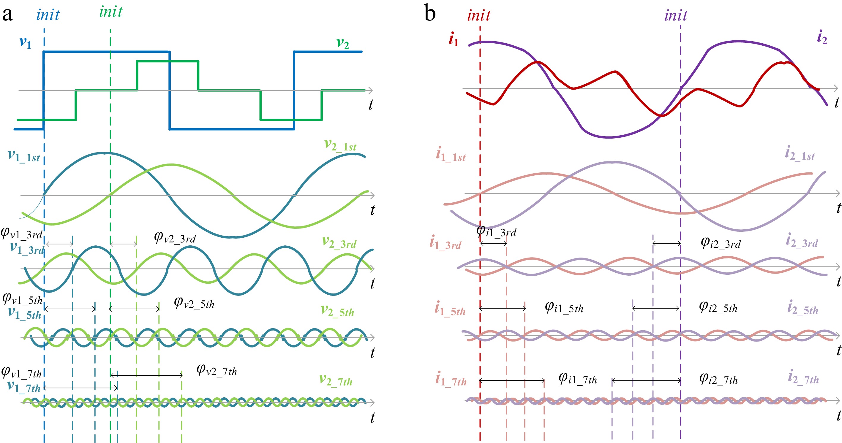
Figure 6.
Phase correction for passive network voltage and current. (a) Voltage v1 and v2. (b) Current i1 and i2.
The passive network current synthesis can be expressed as:
$ {\hat i_1}\left( t \right) = \Im \left( {{{\hat i}_{1\_\varpi }}\left( {t - \dfrac{{{\varphi _{i1\_nth}}}}{{{\omega _c}}}} \right)} \right) $ (30) $ {\hat i_2}\left( t \right) = \Im \left( {{{\hat i}_{2\_\varpi }}\left( {t - \dfrac{{{\varphi _{i2\_nth}}}}{{{\omega _c}}}} \right)} \right) $ (31) $ {\hat i_p}\left( t \right) = \Im \left( {{{\hat i}_{p\_\varpi }}\left( {t - \dfrac{\pi }{{2{\omega _c}}}} \right)} \right),{\hat i_s}\left( t \right) = \Im \left( {{{\hat i}_{s\_\varpi }}\left( {t + \dfrac{\pi }{{2{\omega _c}}}} \right)} \right) $ (32) where, current phase correction ratios φi1_nth, φi2_nth can be expressed as:
$ {\varphi _{i1\_nth}} = \left( {n - 1} \right)\pi \left( {\dfrac{\alpha }{4} - abs(\tilde \kappa \varphi )} \right) $ (33) $ {\varphi _{i2\_nth}} = \left( {n - 1} \right)\pi \left( {1 - \dfrac{\alpha }{4} + \beta - abs(\tilde \kappa \varphi )} \right) $ (34) where, n equals to 1, 3, 5, 7, ···, k is the correction factor used to eliminate the phase impact caused by higher-order harmonics. The current waveforms derived by the FTDC model are shown in Fig. 3 compared with the practical experiment waveforms.
-
In the bidirectional wireless charging system discussed in this paper, it is essential to implement the Power Factor Correction (PFC) function on the network side. This can be achieved by adjusting the inward shift ratio β of the secondary converter. By doing so, the current on the network side can effectively align with the network side voltage, as illustrated in Fig. 7.
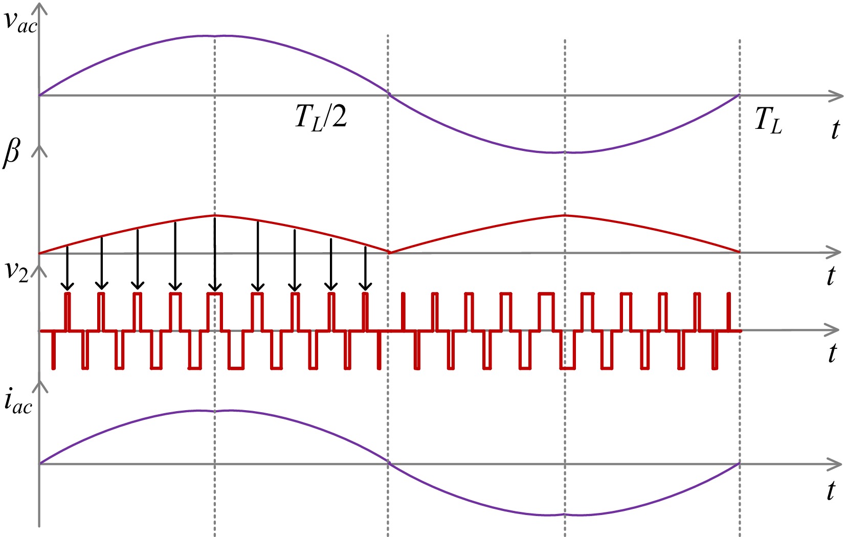
Figure 7.
Waveforms of PFC control using the β regulation method.
The grid side current iac can be obtained by the fundamental wave approximation method[6]
$ {i_{ac}} = \dfrac{{16}}{{{\pi ^2}}}{V_b}\dfrac{M}{{{\omega _0}{L_1}{L_2}}}\sin \left( {\dfrac{\alpha }{2}\pi } \right)\sin \left( {\dfrac{\beta }{2}\pi } \right)\sin \left( {\varphi \pi } \right) $ (35) The control method in this paper is three-shift-ratio regulation control, in which ɑ is 1 as the internal phase shift of the transmitter converter, to ensure that the transmitter converter works in a wide range of Zero Voltage Switching (ZVS). β realizes the PFC function of the system, φ is adjusted to realize the forward and reverse transmission of energy and power regulation.
Figure 8a−c shows the modeling comparison of the BWPT system when φ = 0.5. In Fig. 8a, the voltage and current under FHA are pure sine waves, which cannot be used in the field of accurate modeling; In Fig. 8b, although the TMH modeling has made breakthroughs in current amplitude and voltage shape, there are still problems of phase missing and peak gap. Under TMH, the model is always symmetrical about the center, which does not match the actual current waveform in Fig. 8d, and it is also impossible to accurately calculate the zero-crossing points and amplitude. In Fig. 8c, the FTDC method can ensure the consistency of the amplitude even when vac changes through phase correction, and can achieve good restoration from the perspective of amplitude and phase.per.
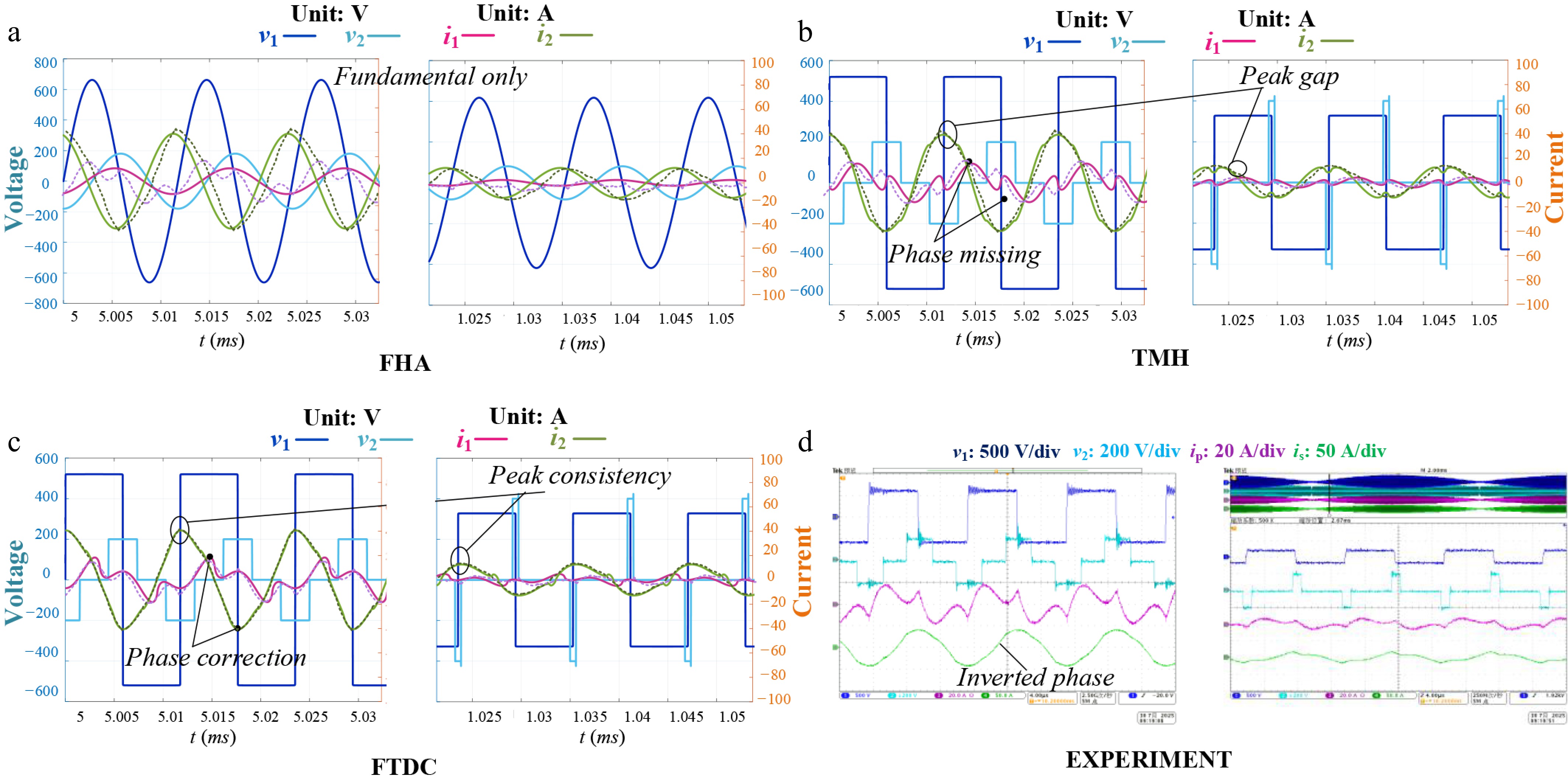
Figure 8.
Theory derivation comparison under φ = 0.5 for G2V (left: max grid voltage vac; right: low grid voltage vac). (a) FHA. (b) TMH. (c) FTDC. (d) Experiment.
The theoretical voltage and current waveforms illustrated in Fig. 9 can be derived using the FTDC analysis method. In Fig. 9a−d, the left figures depict the transient voltage and current waveforms of the passive network when the network side voltage is at its maximum. Conversely, the right figures show the corresponding waveforms when the grid side voltage is low.
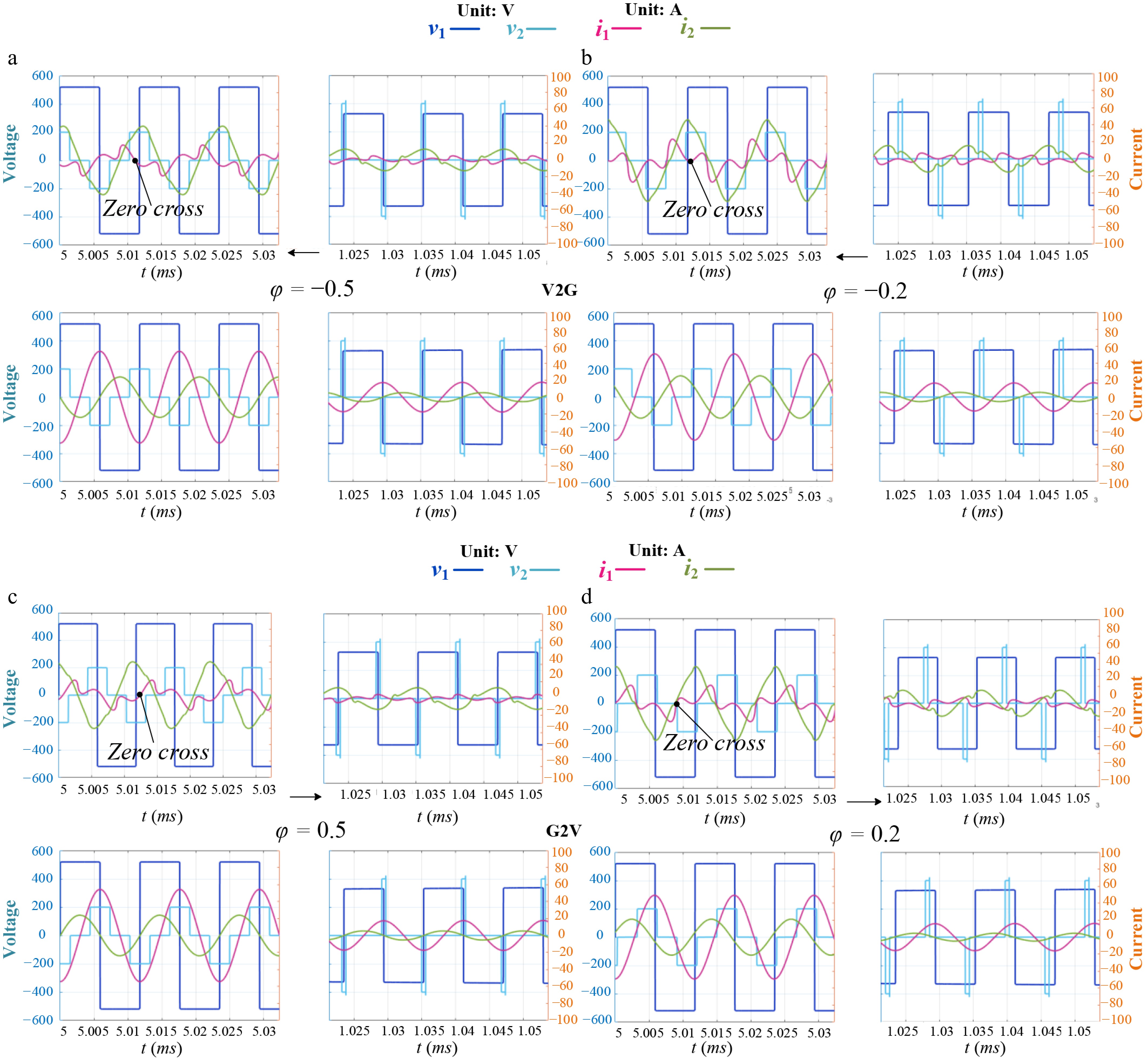
Figure 9.
Theory derivation of voltage and current in steady state (left: max vac; right: low vac). (a) φ = −0.5 for V2G. (b) φ = −0.2 for V2G. (c) φ = 0.5 for G2V. (d) φ = 0.2 for G2V.
The coil currents ip and is are sinusoidal, making it straightforward to extract their amplitude and phase information. Based on the theoretical data, key parameters such as the peak-to-peak value, effective value, and zero-crossing points of ip and is can be easily calculated. While i1 is equivalent to i2, it is important to note that due to the unique characteristics of the LCC compensation network, i1 and i2 are non-sinusoidal. However, the waveform reconstructed using the FTDC method still closely resembles the expected shape. In addition to the amplitude, the zero-crossing points are clearly identifiable, and the effective value of the current can be computed using discrete integration.
$ {\hat X_{pos\_RMS}} = \sqrt {\dfrac{1}{T}} \sum {\hat x_{pos}^2(t)} {t_{step}} $ (36) $ {\hat X_{pos\_Ap}} = \max (abs({\hat x_{pos}}(t))) $ (37) $ {\hat T_{zero}} = Solve({\hat x_{pos}}(t) = 0) $ (38) where, xpos represents i1, i2, ip, and is. Root Mean Square (RMS) value Xpos_RMS, amplitude value Xpos_Ap, zero crossing point Tzero can be represented by Eqs (36)–(38). T is the period, and tstep is the time step. At the same time, according to the above data, the soft switching state of the converter can also be judged. For example, the relationship between v1 and i1 indicates that the primary side converter works in ZVS state.
-
Figure 10 shows the BWPT system experiment test bench based on the single-stage totem pole AC-AC converter.
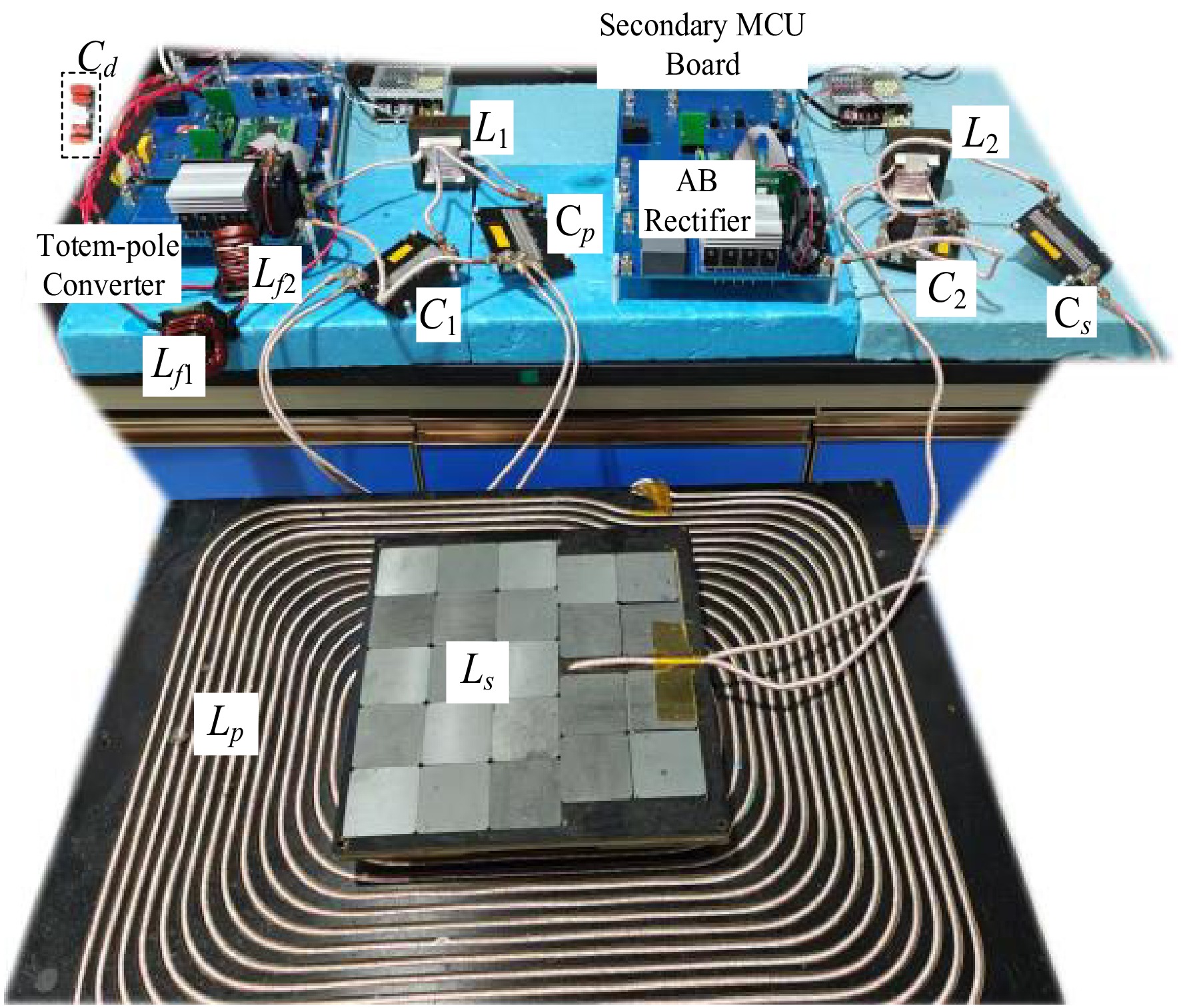
Figure 10.
BWPT system experiment test bench.
Figure 11a and b illustrate the voltage and current waveforms at the network side, as well as the voltage waveforms at the primary and secondary sides of the passive network. The primary side input voltage v1 varies in response to the grid side voltage, while the amplitude of the secondary side voltage v2 is influenced by the load voltage.
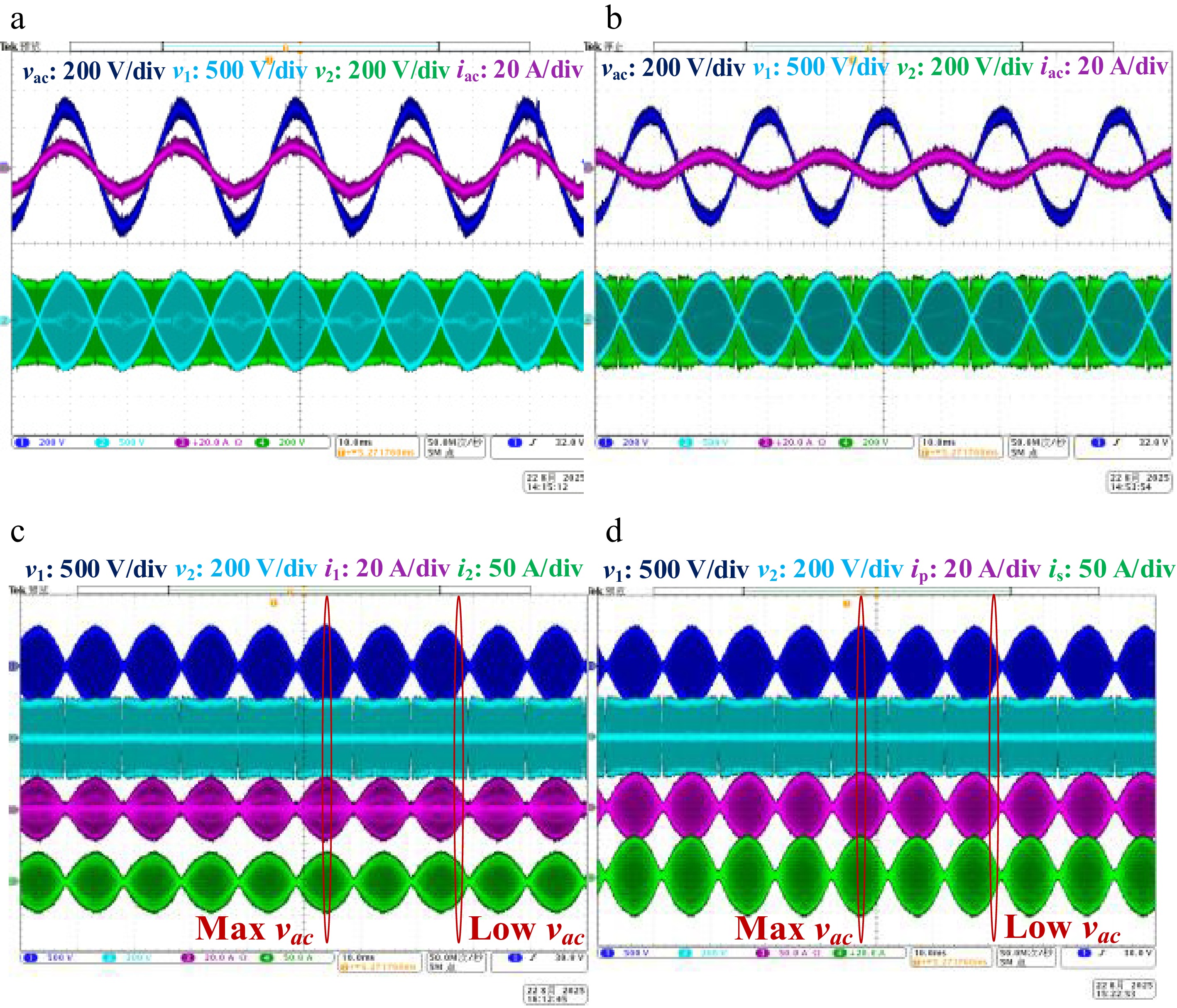
Figure 11.
Specific experiment waveforms of BWPT system. (a) φ = 0.5 for G2V. (b) φ = −0.3 for V2G. (c) Steady-state waveforms with i1 and i2. (d) Steady-state waveforms with ip and is.
Figure 12 corresponds to Fig. 9a, Fig. 13 to Fig. 9b, Fig. 14 to Fig. 9c, and Fig. 15 to Fig. 9d. The dashed lines '---' in Figs 12−15 are depicted from the theoretical results in Fig. 9. The phase difference between the primary and secondary side voltages v1 and v2 is represented by a shift of φ. The left images correspond to the passive network waveforms when the grid voltage vac is at its maximum, while the right images represent the waveforms when the grid voltage vac is low.
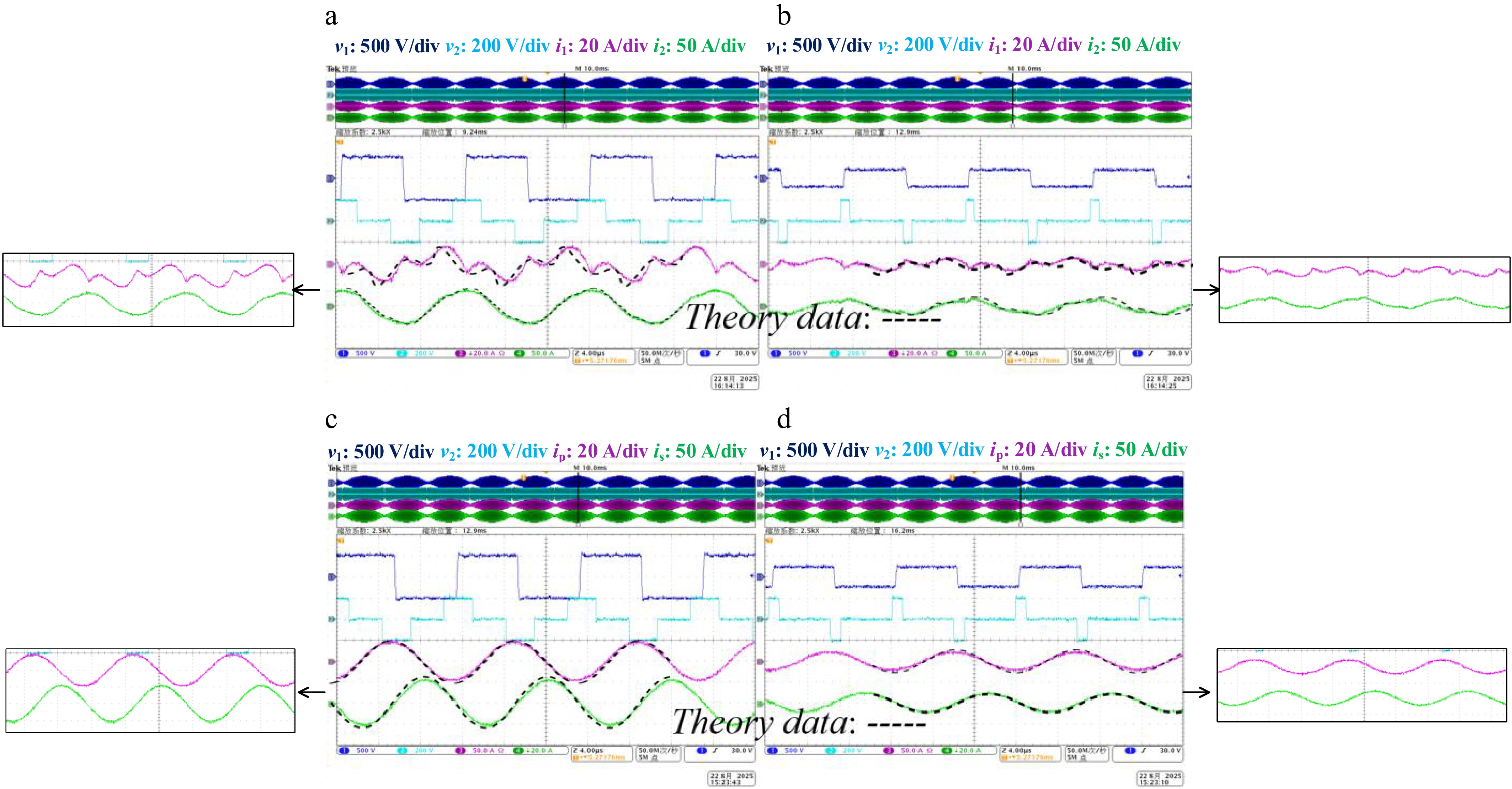
Figure 12.
Experiment validation of φ = −0.5 for V2G. (a) Maximum vac with i1 and i2. (b) Low vac with i1 and i2. (c) Steady-state waveforms with ip and is. (d) Low vac with ip and is.
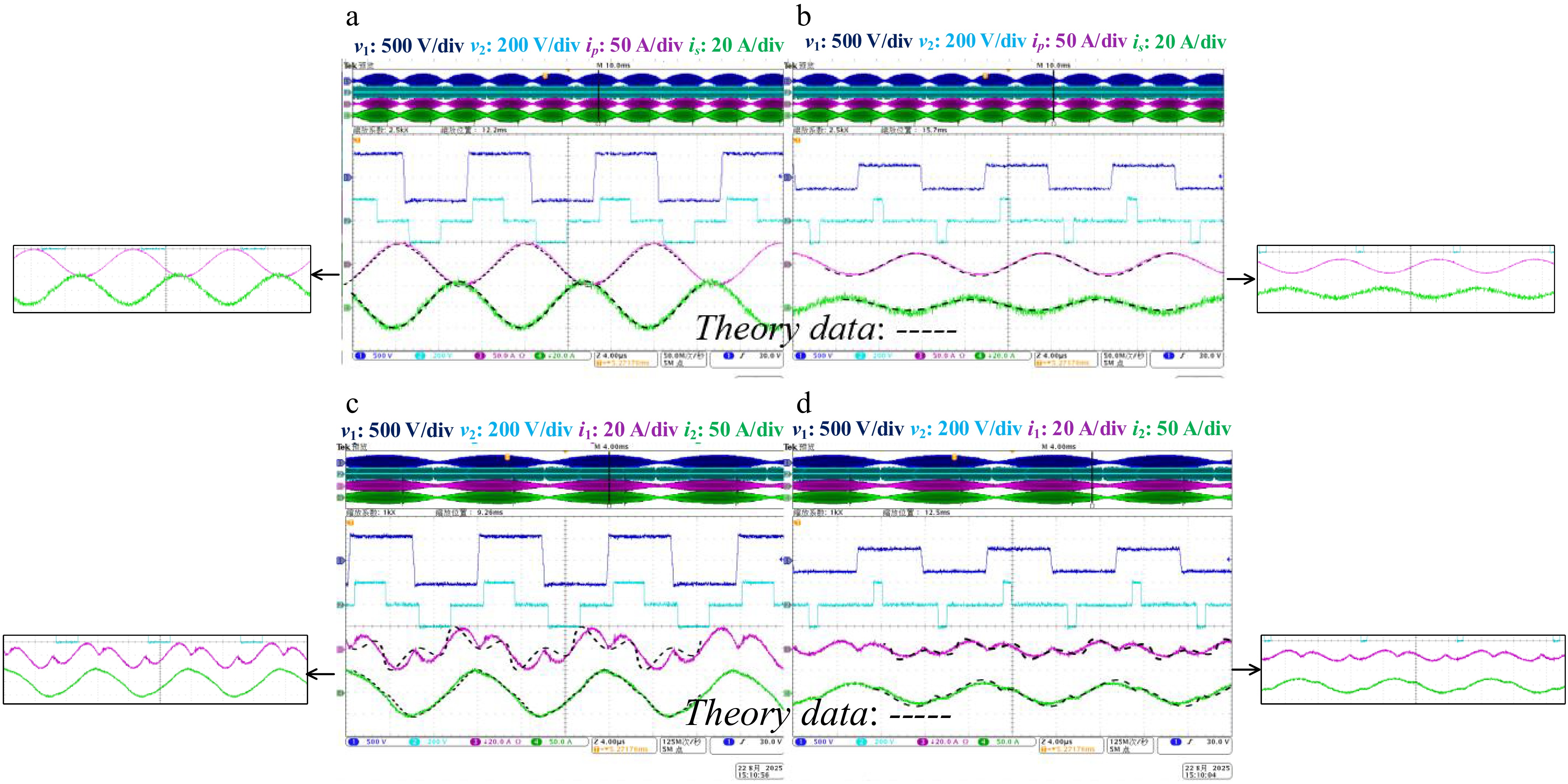
Figure 13.
Experiment validation of φ = −0.2 for V2G. (a) Maximum vac with i1 and i2. (b) Low vac with i1 and i2. (c) Maximum vac with ip and is. (d) Low vac with ip and is
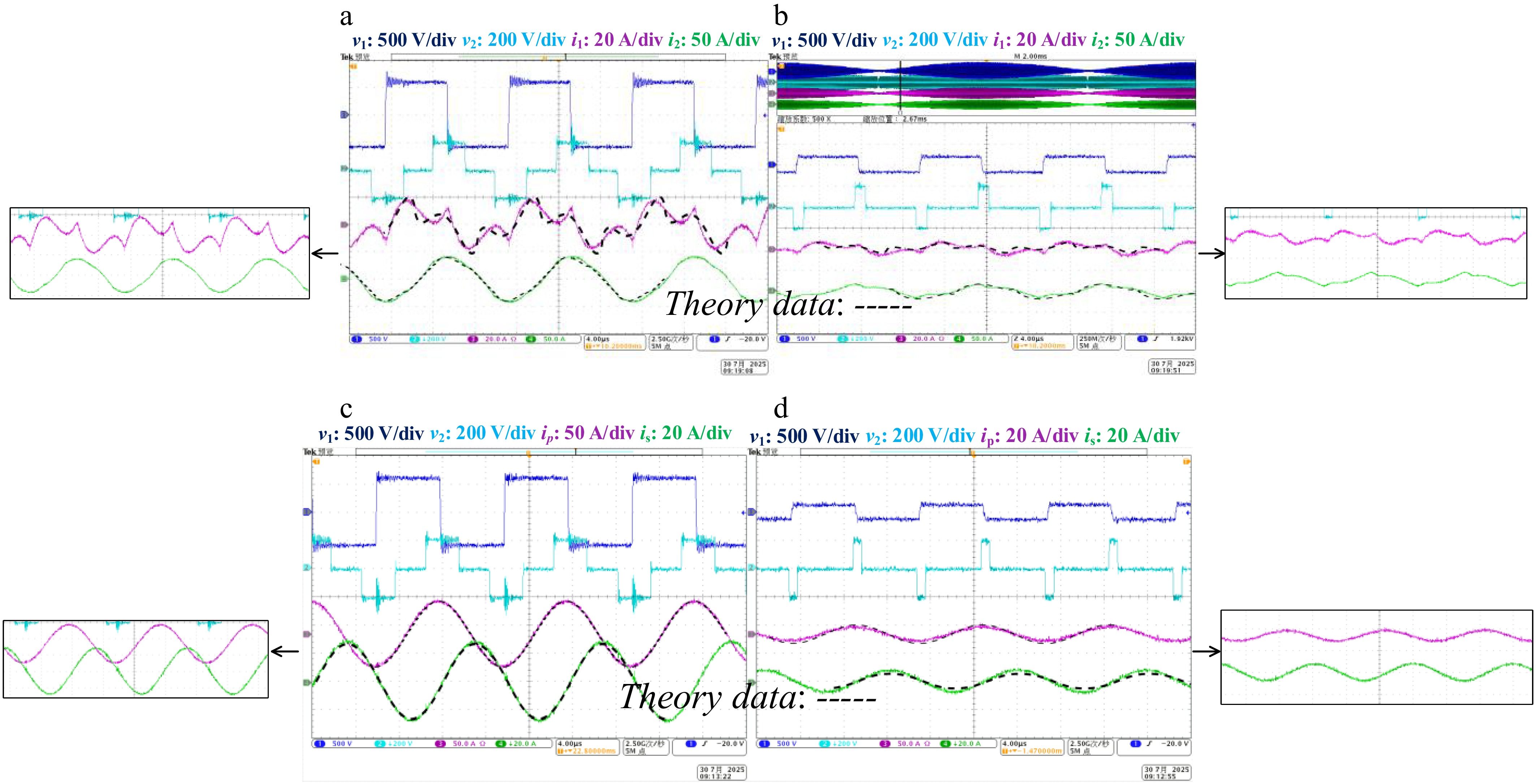
Figure 14.
Experiment validation of φ = 0.5 for G2V. (a) Maximum vac with i1 and i2. (b) Low vac with i1 and i2. (c) Maximum vac with ip and is. (d) Low vac with ip and is.
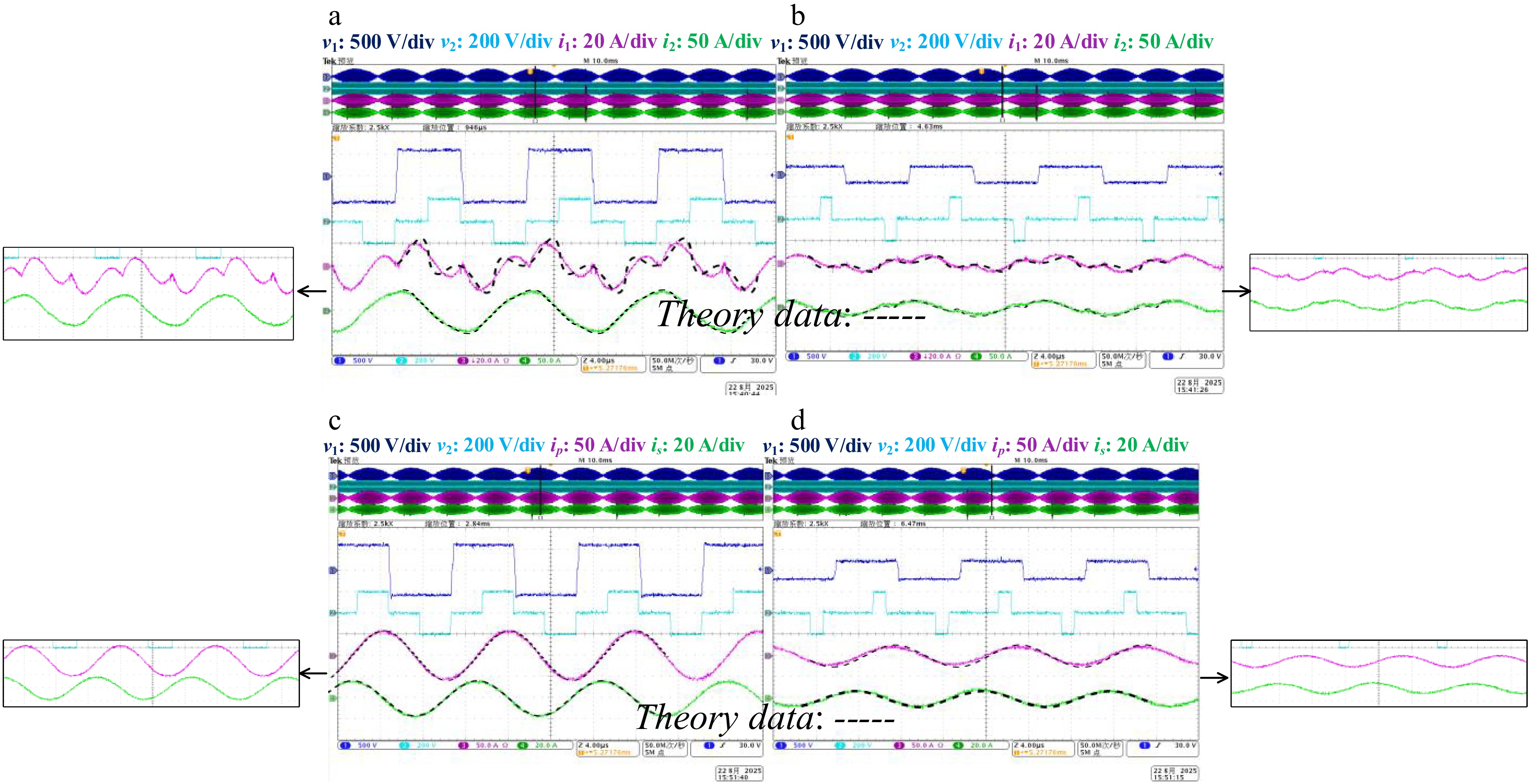
Figure 15.
Experiment validation of φ = 0.2 for G2V. (a) Maximum vac with i1 and i2. (b) Low vac with i1 and i2. (c) Maximum vac with ip and is. (d) Low vac with ip and is.
The displayed waveforms demonstrate that the waveforms obtained through the FTDC theory (shown as dashed lines) closely align with those derived from actual experiments across a wide range of operating points. The primary input current i1 exhibits a slight deviation in shape; this discrepancy arises from the interplay between the frequency and time domains, where the derivation of frequency domain impedance is the primary consideration. Consequently, it becomes challenging to accurately capture the waveform variations within a single cycle. Nonetheless, the final amplitude, effective value, and zero-crossing points show strong agreement with experimental results, thereby validating the effectiveness of the FTDC method.
The FTDC method integrates both time-domain and frequency-domain analysis techniques. Essentially, the final voltage and current waveforms are derived by superimposing sinusoidal waves over the complete period of each harmonic. As a result, there may be slight discrepancies in shape when compared to experimental waveforms. However, in terms of amplitude, phase, effective value, and zero-crossing points, the FTDC method proves to be more suitable for experimental applications. However, under the TMH method, the calculation of the peak has a significant deviation, not to mention the FHA method. As the phase shift ratio φ decreases, the gap between the theoretical value and the actual value becomes larger.
Figure 16 shows the comparison between theoretical and experimental current error data when the grid-side voltage vac reaches its maximum. The current error err is defined as:
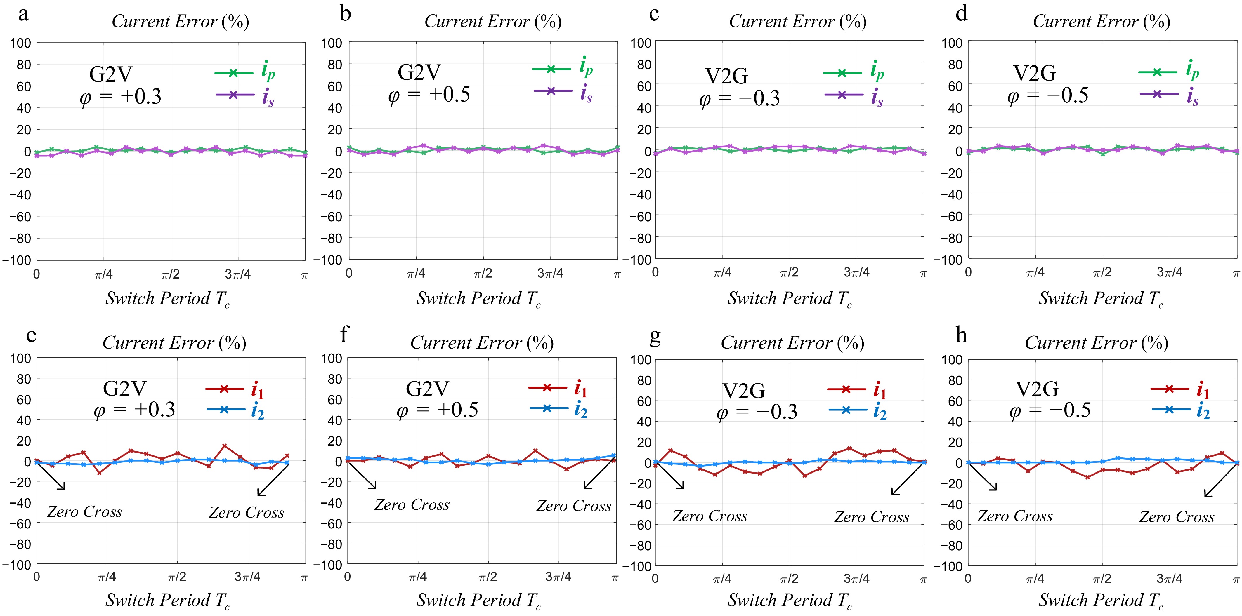
Figure 16.
The error of passive network currents under different phase shifts and different power transfer directions. (a) ip and is for φ = +0.3. (b) ip and is for φ = +0.5. (c) ip and is for φ = −0.3. (d) ip and is for φ = −0.5. (e) i1 and i2 for φ = +0.3. (f) i1 and i2 for φ = +0.5. (g) i1 and i2 for φ = −0.3. (h) i1 and i2 for φ = −0.5.
$ err = \dfrac{{{i_{exp}} - {i_{thy}}}}{{{i_{pp\_exp}}}} \times 100{\text{%}} $ (39) where, iexp is experiment current, ithy is theoretical calculation current, ipp_exp is peak-peak experiment current.
The current errors of i2, ip, is are guaranteed to stay within 5%, reflecting the accuracy of the FTDC analysis method. However, the error for i1 is relatively larger. This is mainly due to a phase shift between the peak value and the actual comparison. Nevertheless, the error remains within 20%, and the zero-crossing errors for both i1 and i2 can be kept within 5%. Therefore, based on these theoretical results, the soft-switching status of the switch tubes can be accurately determined.
The results above can also be validated by Fig. 17, which demonstrates that the results from the FTDC theory closely reflect the experimental outcomes, thus effectively achieving the goal of waveform prediction.
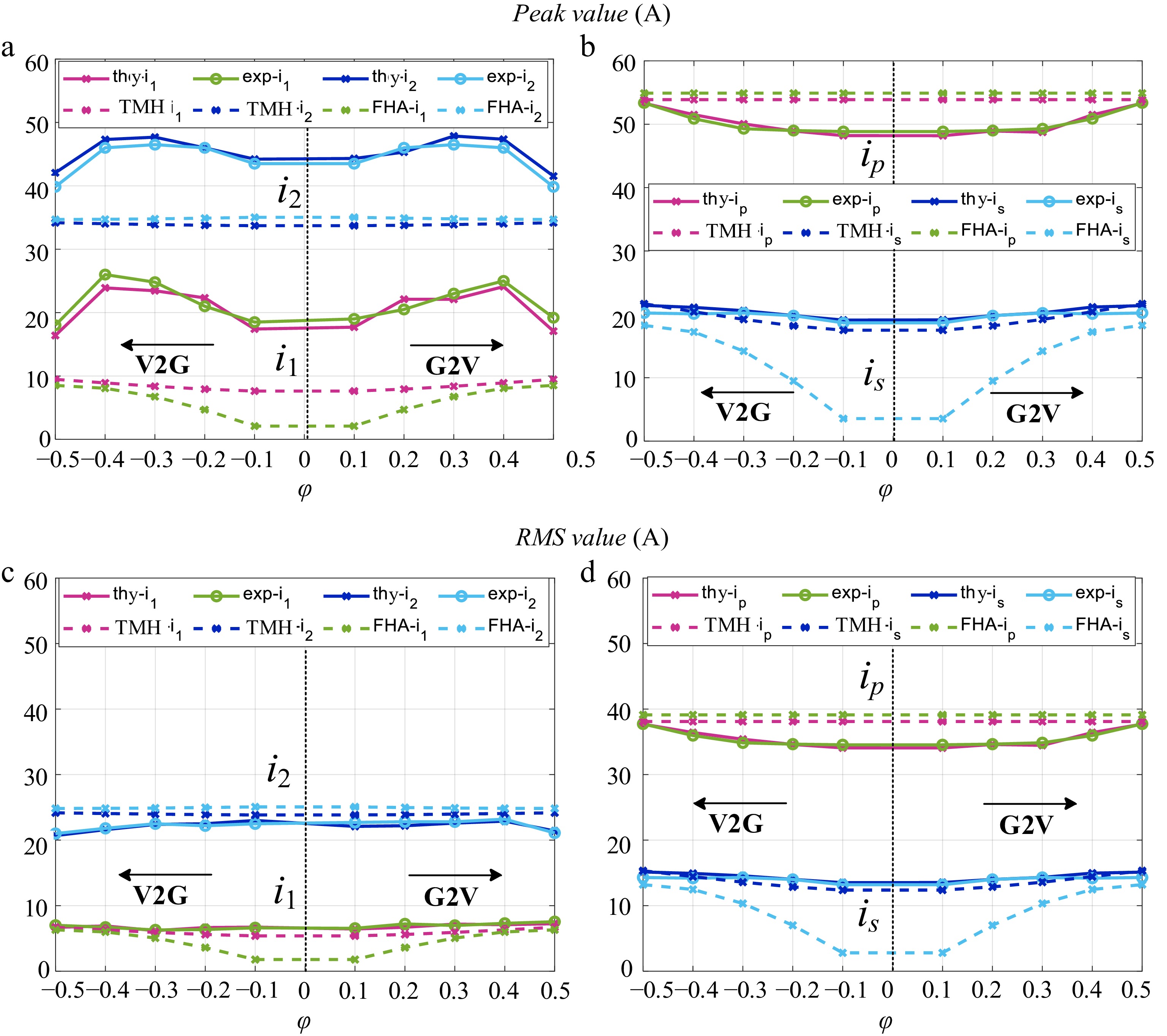
Figure 17.
Experiment validation data ('thy' for 'theory', 'exp' for 'experiment'). (a) i1 and i2 for amplitude. (b) ip and is for amplitude. (c) i1 and i2 for RMS value. (d) ip and is for RMS value.
Tables 3 and 4 present detailed data of FTDC calculation and experiment from Figs 16 and 17 with φ = +0.5 and φ = −0.1.
Table 3. Detailed data of FTDC calculation and experiment with φ = +0.5.
Method type Peak value (A) RMS value (A) Mean value of current error i1 i2 ip is i1 i2 ip is i1 i2 ip is FHA 9.1 34.8 55.8 17.6 7.6 25.1 39.8 13.3 / / / / TMH 9.8 34.4 55.5 20.9 8.2 24.6 38.5 15.6 / / / / thy(FTDC) 17.7 42.0 55.3 20.9 8.3 20.6 38.4 15.5 7.8% 2.1% 1.2% 1.9% exp(Experiment) 19.6 39.9 55.3 20.0 8.3 20.6 38.4 14.7 Table 4. Detailed data of FTDC calculation and experiment with φ = −0.3.
Method type Peak value (A) RMS value (A) Mean value of current error i1 i2 ip is i1 i2 ip is i1 i2 ip is FHA 4.8 35 55.8 14.2 5.8 24.9 39.8 10.2 / / / / TMH 9.2 34.7 54.9 19.3 6.2 23.6 37.9 13.6 / / / / thy(FTDC) 23.3 47.9 50.0 20.3 6.3 22.8 35.5 14.8 12.2% 2.3% 1.7% 1.8% exp(Experiment) 24.8 46.1 49.7 20.2 6.2 22.8 35.3 14.7 Table 5 presents a comparison of different WPT modeling methods. FHA, Generalized Space-State Averaging (GSSA), TMH, and sample-data model[11] all focus on obtaining the average state of the system, with ample-data model being applicable only to Series-Series (SS) topologies and unidirectional energy transfer applications. Methods of time-domain analysis[12−13] employ complex frequency domain analysis, with discrete-time model[13] specifically designed for DLCC systems but not supporting BWPT systems. The approach outlined in this paper, however, not only models the system characteristics in both G2V and V2G directions but also achieves a lower-order representation, ensuring both a manageable computational load and accurate results.
Table 5. Comparison between various methods in WPT application.
Method type Amount of calculation Number of order n BWPT
supportComputational complexity Compensation network Three feature outputs Accuracy (for
feature outputs)FHA Small 1 Yes Simple Unrestricted Average only Low GSSA Large Infinite Yes Very complex Unrestricted Average only High TMH analysis[18−20] Medium Not mentioned No Medium Unrestricted All Medium Sample-data model[21] Large Infinite No Complex SS Average only Very high harmonics-considered
time-domain model[22]Small Not mentioned No Medium Unrestricted All Medium Discrete-time model[23] Very large 9 No Complex DLCC All Very high Proposed FTDC Medium 3, 9 Yes Medium Unrestricted All High -
To address the result deviation caused by primary-secondary phase difference when using the TMH method, this paper presents an FTDC analysis prediction method for the BWPT system using a single-stage totem-pole AC-AC converter. First, it analyzes the harmonics composition of the input and output voltage and current within the passive network, providing expressions for each component of the passive impedance like the TMH method. Then, the harmonics reconstruction based on the phase correction of the voltage and current variables are derived using the homogeneous and superposition theorems. Theoretical expressions and waveforms for voltage and current are then obtained by combining both frequency-domain and time-domain methods. Experimental results are used to validate the consistency between the theoretical and measured waveforms. Additionally, the paper investigates deviations in current amplitude, effective value, phase, and zero-crossing points compared to experimental data, confirming the accuracy of the proposed analytical method. Finally, for the complex system of a single-stage AC-AC converter in the BWPT setup, the FTDC analysis method effectively provides accurate theoretical results across various operating points.
-
The authors confirm contribution to the paper as follows: study conception and design: Zhang X, Zhang Q, Wu H, Dong S; data collection: Zhang X; software: Zhang X; validation: Zhang X, Zhang Q; analysis and interpretation of results: Zhang X, Zhang Q, Wu H, Dong S; draft manuscript preparation: Zhang X, Zhang Q, Wu H, Dong S; supervision: Zhang Q. All authors reviewed the results and approved the final version of the manuscript.
-
All data that support the findings of this study are available upon reasonable request from the corresponding author.
-
The authors declare that they have no conflict of interest.
- Copyright: © 2025 by the author(s). Published by Maximum Academic Press, Fayetteville, GA. This article is an open access article distributed under Creative Commons Attribution License (CC BY 4.0), visit https://creativecommons.org/licenses/by/4.0/.
-
About this article
Cite this article
Zhang X, Zhang Q, Wu H, Dong S. 2025. Frequency-time domain combined analysis method for bidirectional wireless power transfer system based on single-stage AC-AC converter. Wireless Power Transfer 12: e033 doi: 10.48130/wpt-0025-0032 

Frequency-time domain combined analysis method for bidirectional wireless power transfer system based on single-stage AC-AC converter
- Received: 31 July 2025
- Revised: 08 September 2025
- Accepted: 08 October 2025
- Published online: 25 December 2025
Abstract: The First-Harmonic Approximation (FHA) analysis method is widely utilized in Bidirectional Wireless Power Transfer (BWPT) systems, providing simplified input and output characteristics. However, in complex systems and varying operating conditions, such as those involving a single-stage AC-AC converter, the FHA method falls short, leading to significant calculation deviations that fail to accurately represent the system's working state, as the same as Traditional Multi-harmonics methods (TMH), and time-domain only derivation methods. This paper introduces a novel Frequency-Time Domain Combined (FTDC) analysis prediction method that enhances the precision of the system's operational analysis through theoretical calculations. The proposed method integrates frequency domain analysis with time domain analysis to reconstruct the system's voltage and current waveforms via data deduction and iteration. Notably, this approach outperforms simulation software by rapidly yielding the steady-state waveform and directly providing essential data, including Root Mean Square (RMS) values, amplitude values, and zero-crossing points. This efficiency aids in the expedited and improved design of the entire BWPT system. Finally, the accuracy and practicality of the proposed method are validated through a combination of theoretical analysis and experimental results.
-
Key words:
- BWPT /
- Single-stage /
- FHA /
- TMH /
- Prediction