-
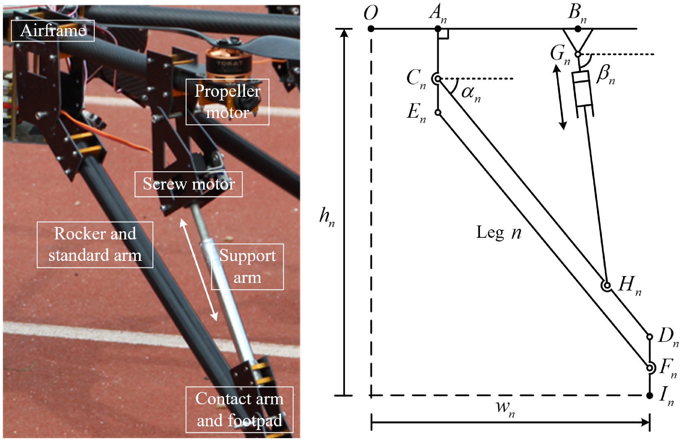
Figure 1.
Single rocker-actuated landing leg.
-
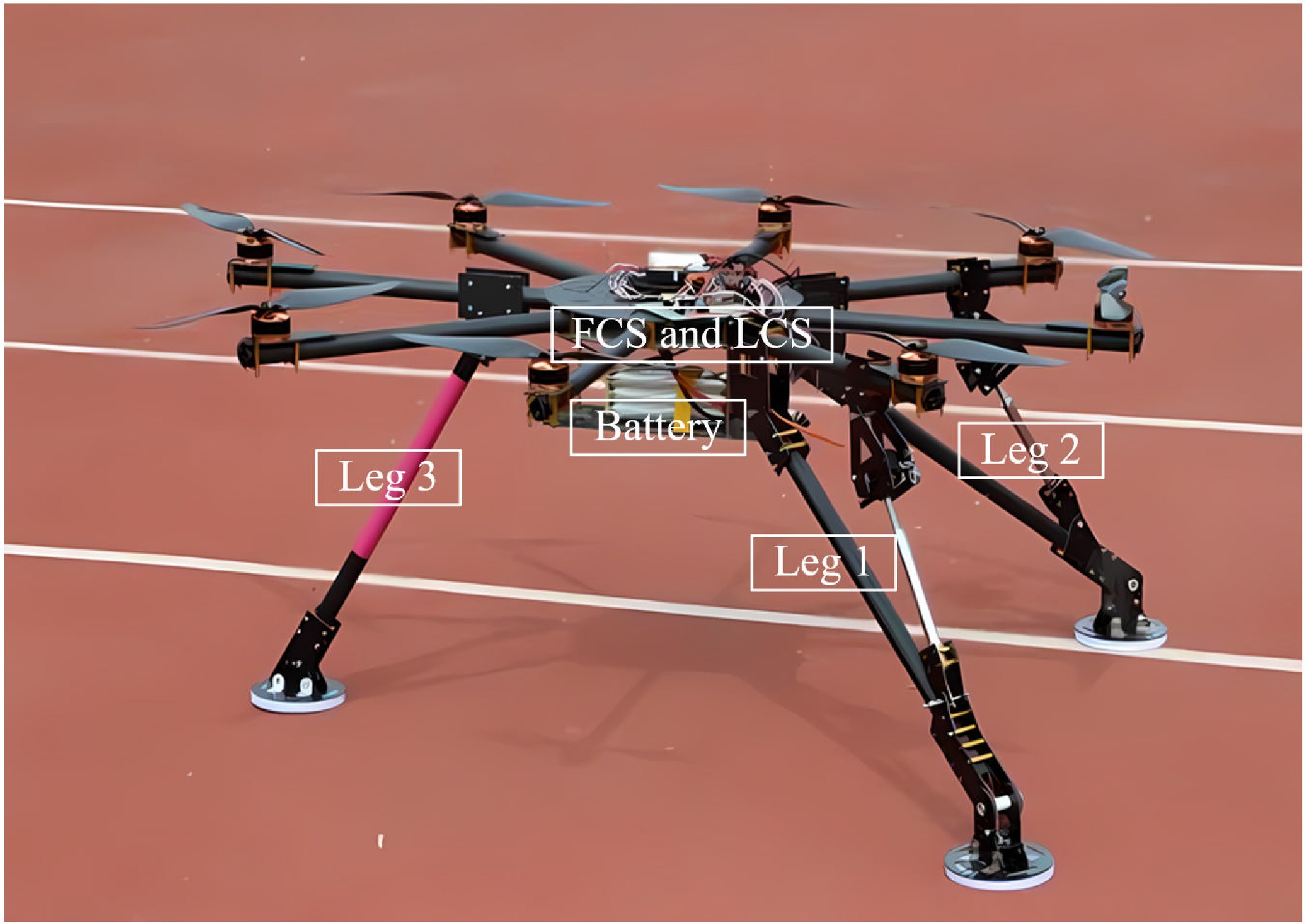
Figure 2.
Movable legs (Nos. 1−2, black) and fixed leg (No. 3, red).
-
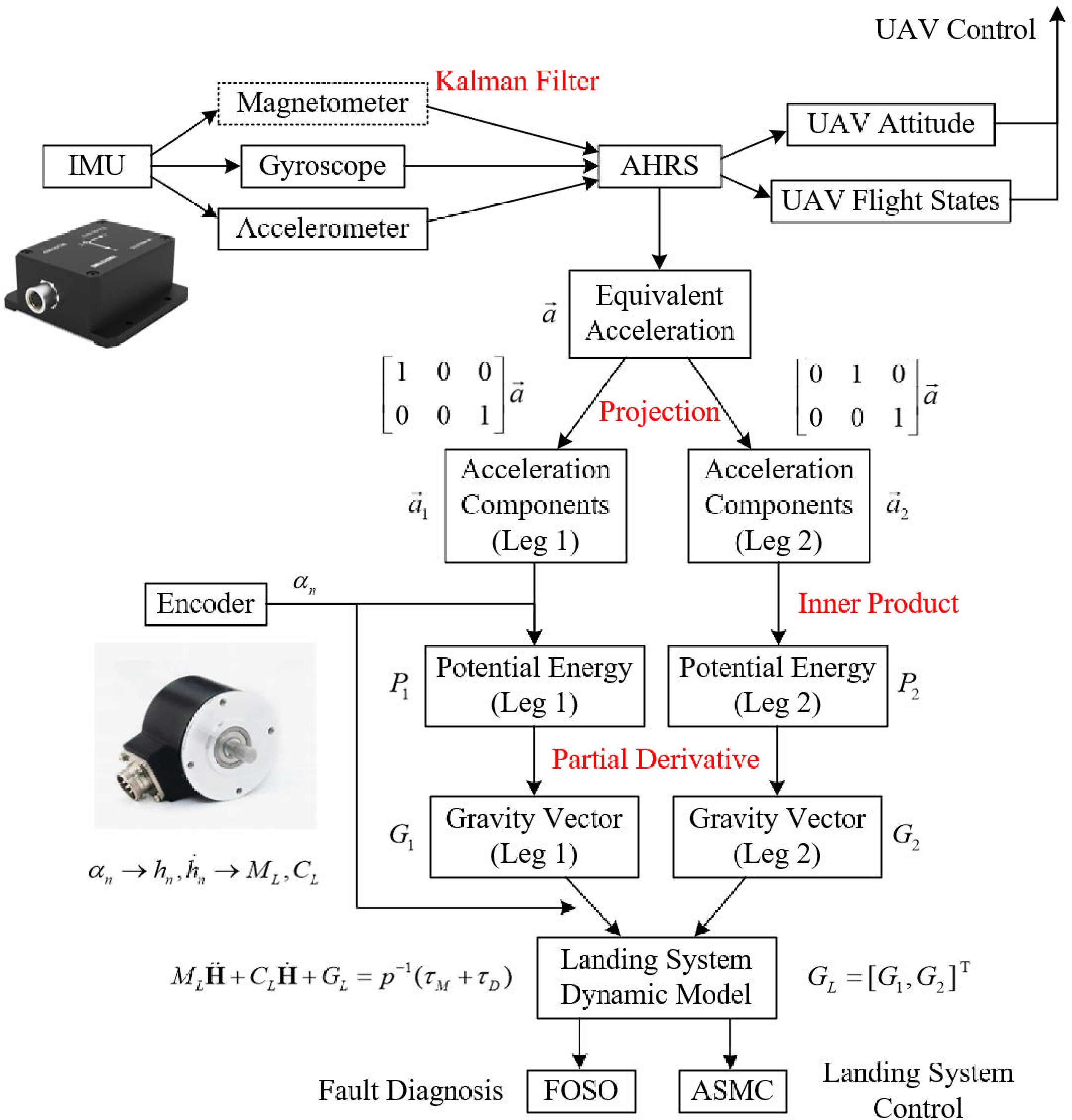
Figure 3.
Dynamic model solution for the landing system.
-
Figure 4.
Dynamic perception strategy for the landing model.
-
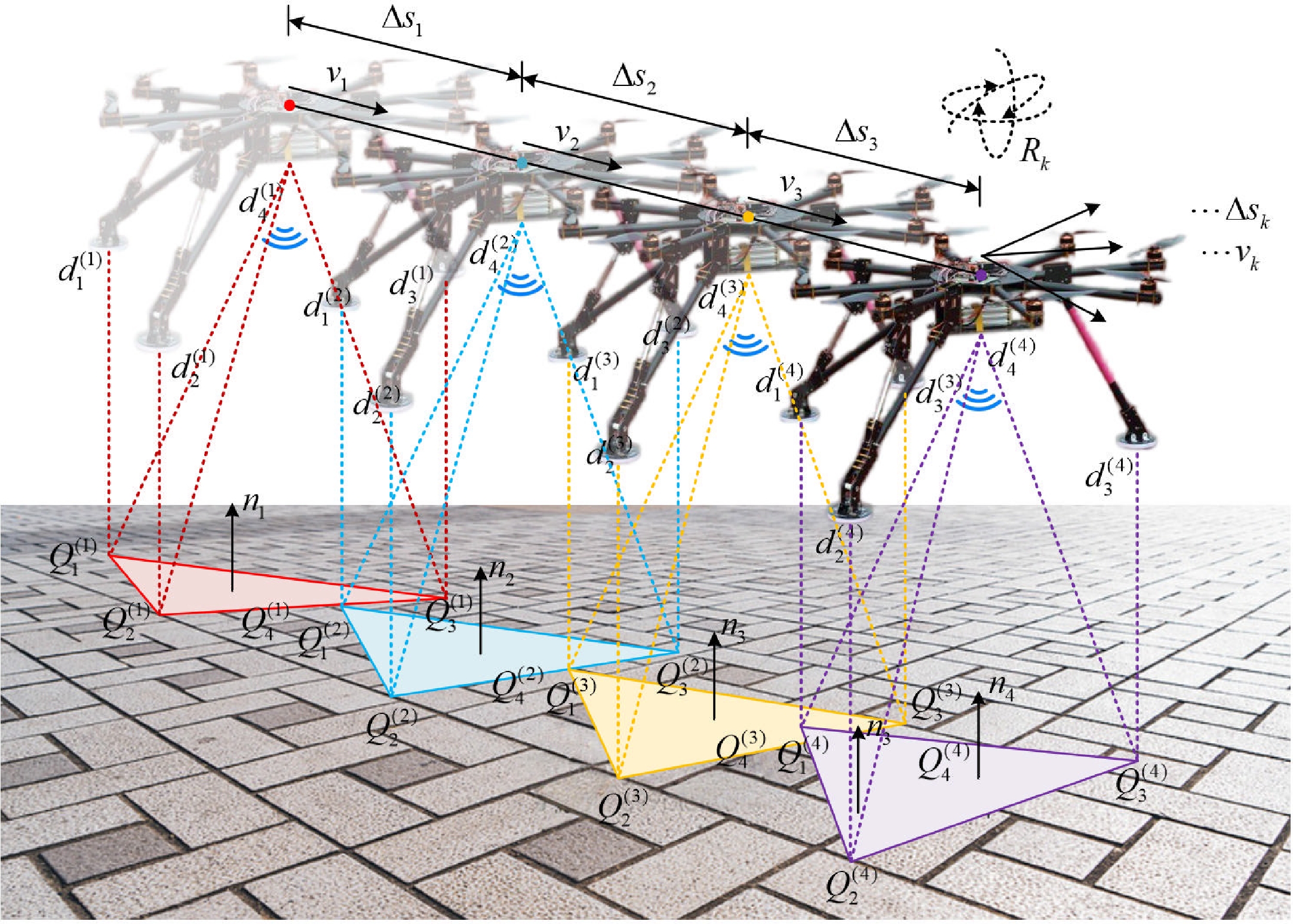
Figure 5.
Schematic diagram of the DTFSF method.
-
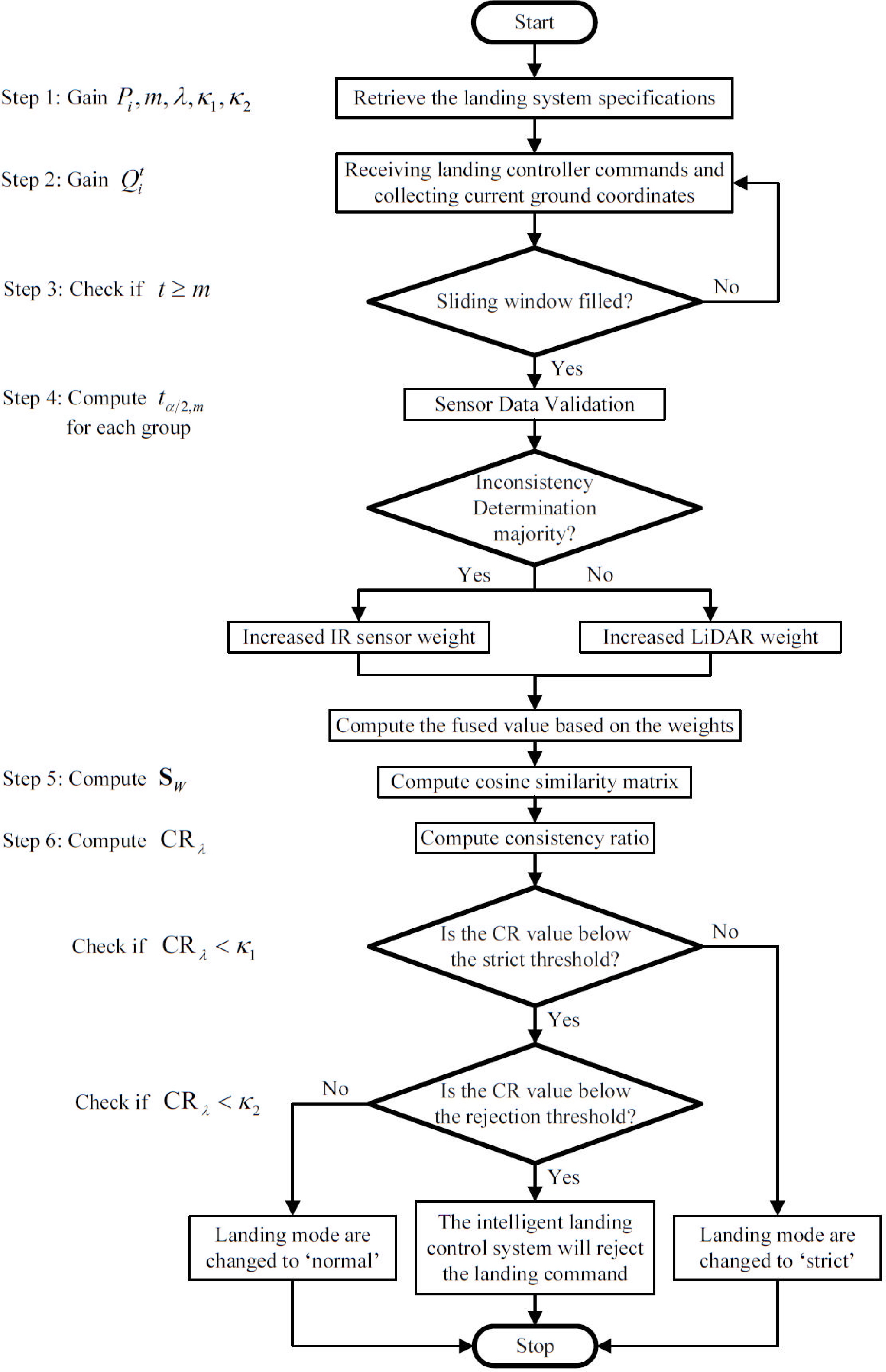
Figure 6.
Flowchart of the DTFSF method.
-
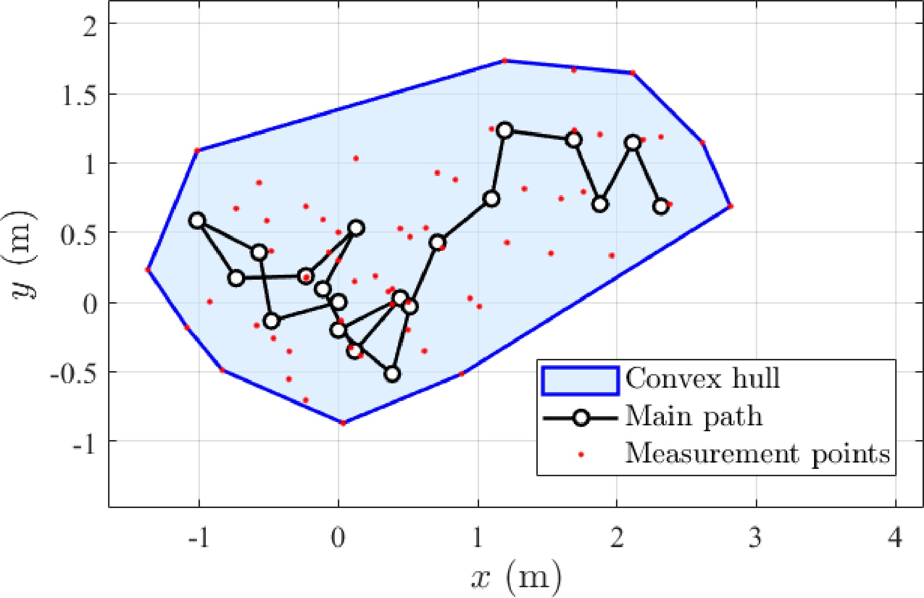
Figure 7.
Illustration of a randomized path (m = 20).
-
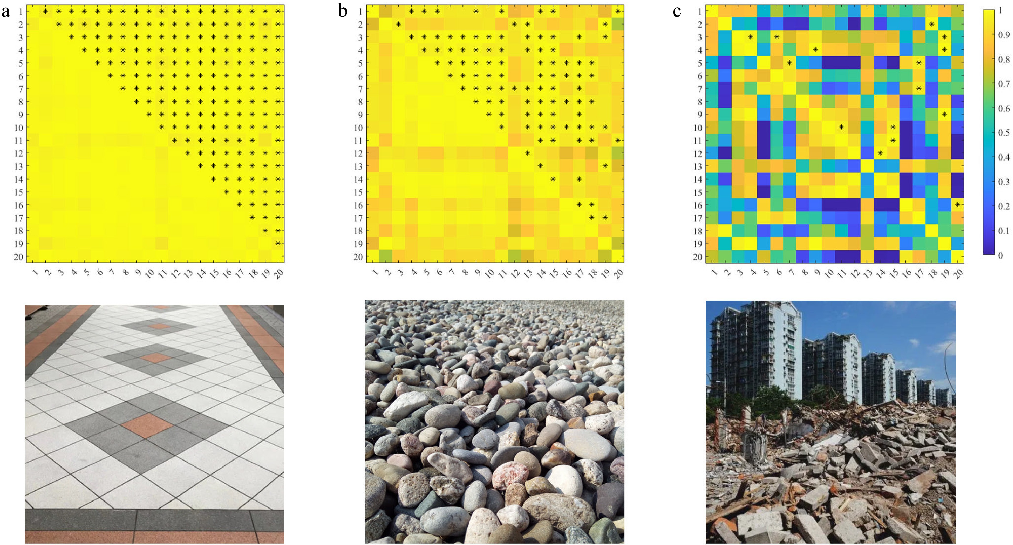
Figure 8.
Landing terrain types and the corresponding CSM: (a) Basic, (b) obstacle, and (c) extreme.
-
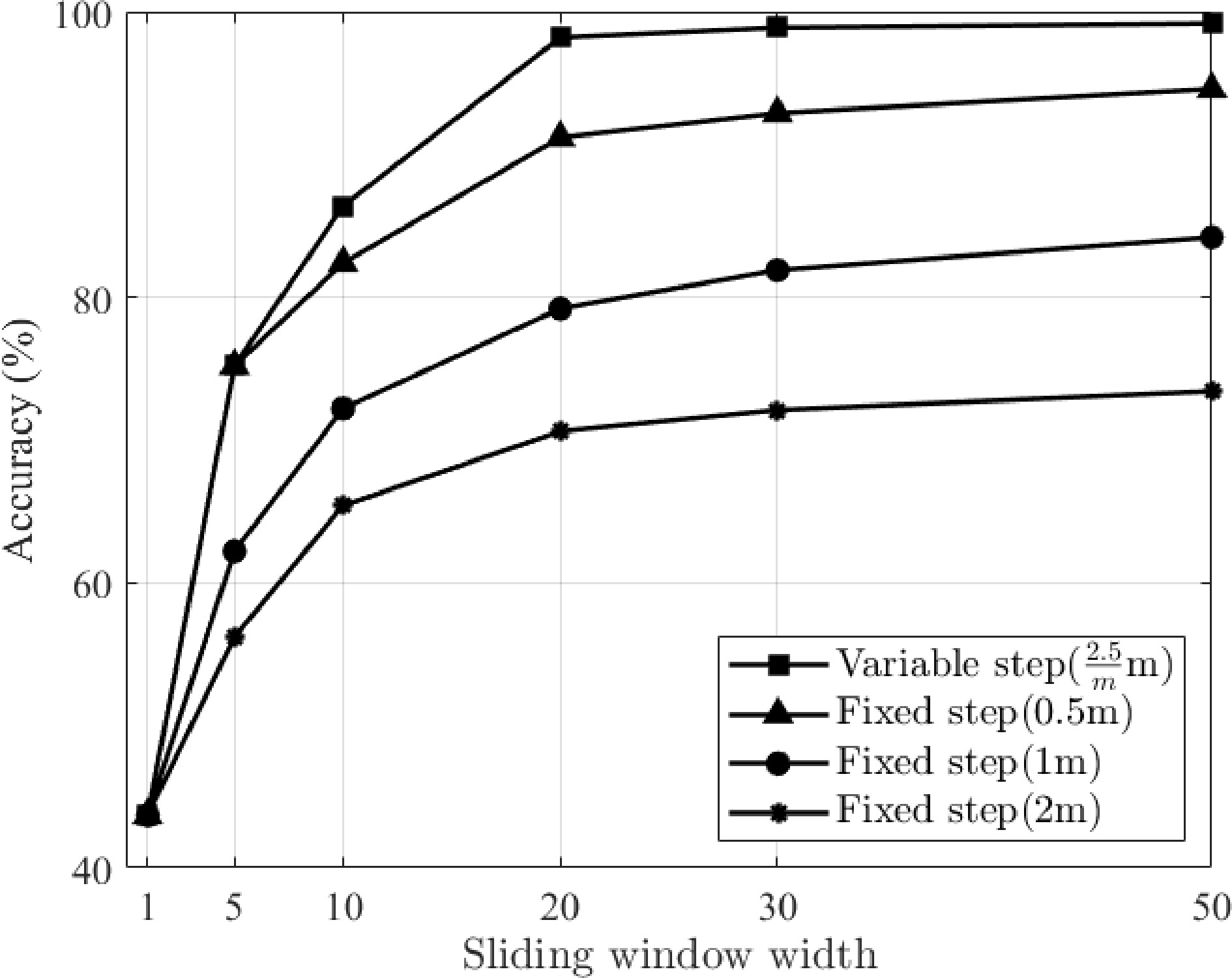
Figure 9.
Recognition accuracy at different step sizes.
-
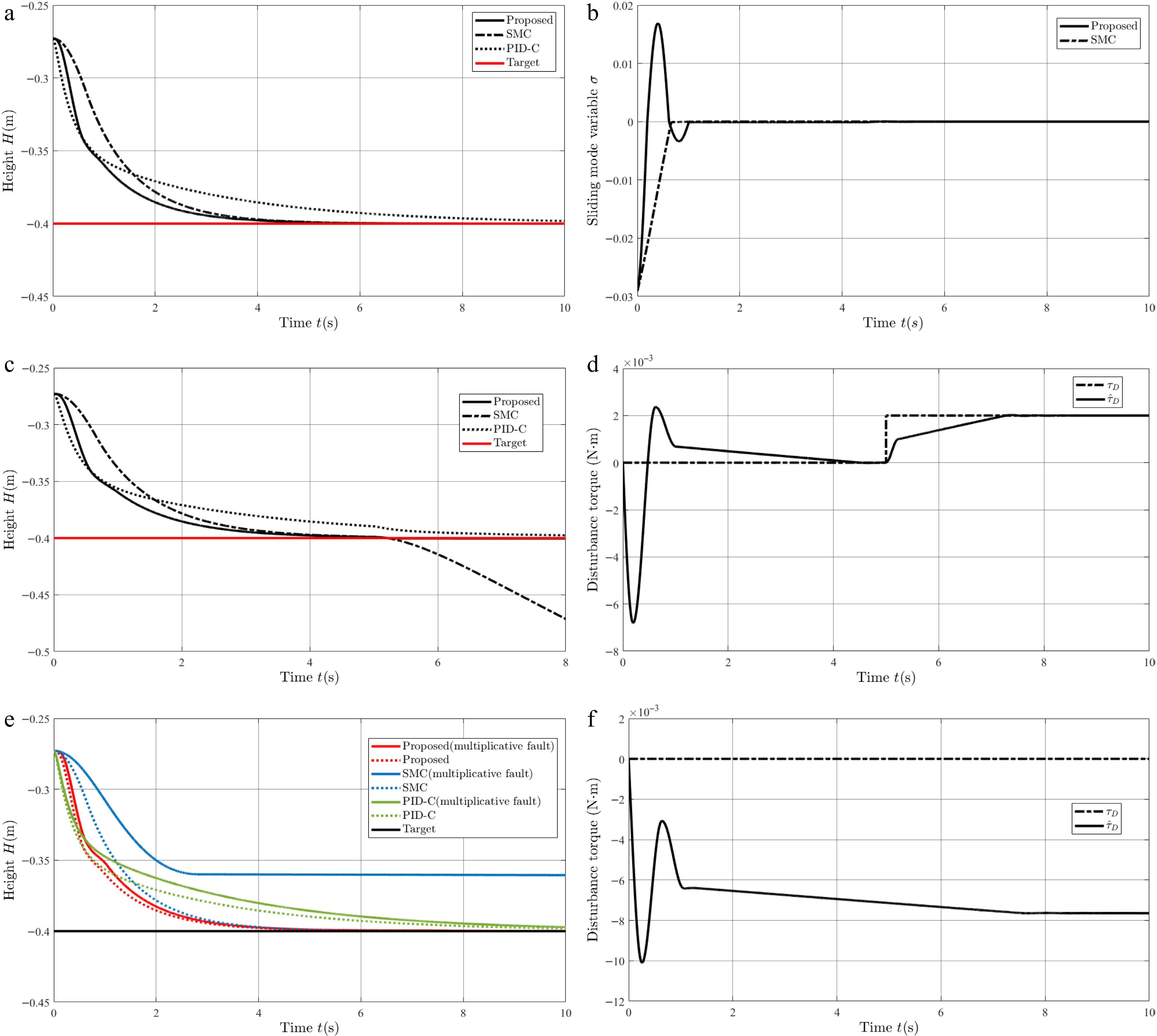
Figure 10.
Simulation results: (a) H for Case 1; (b)
$ \sigma $ $ {\hat{\tau }}_{D} $ $ {\hat{\tau }}_{D} $ -
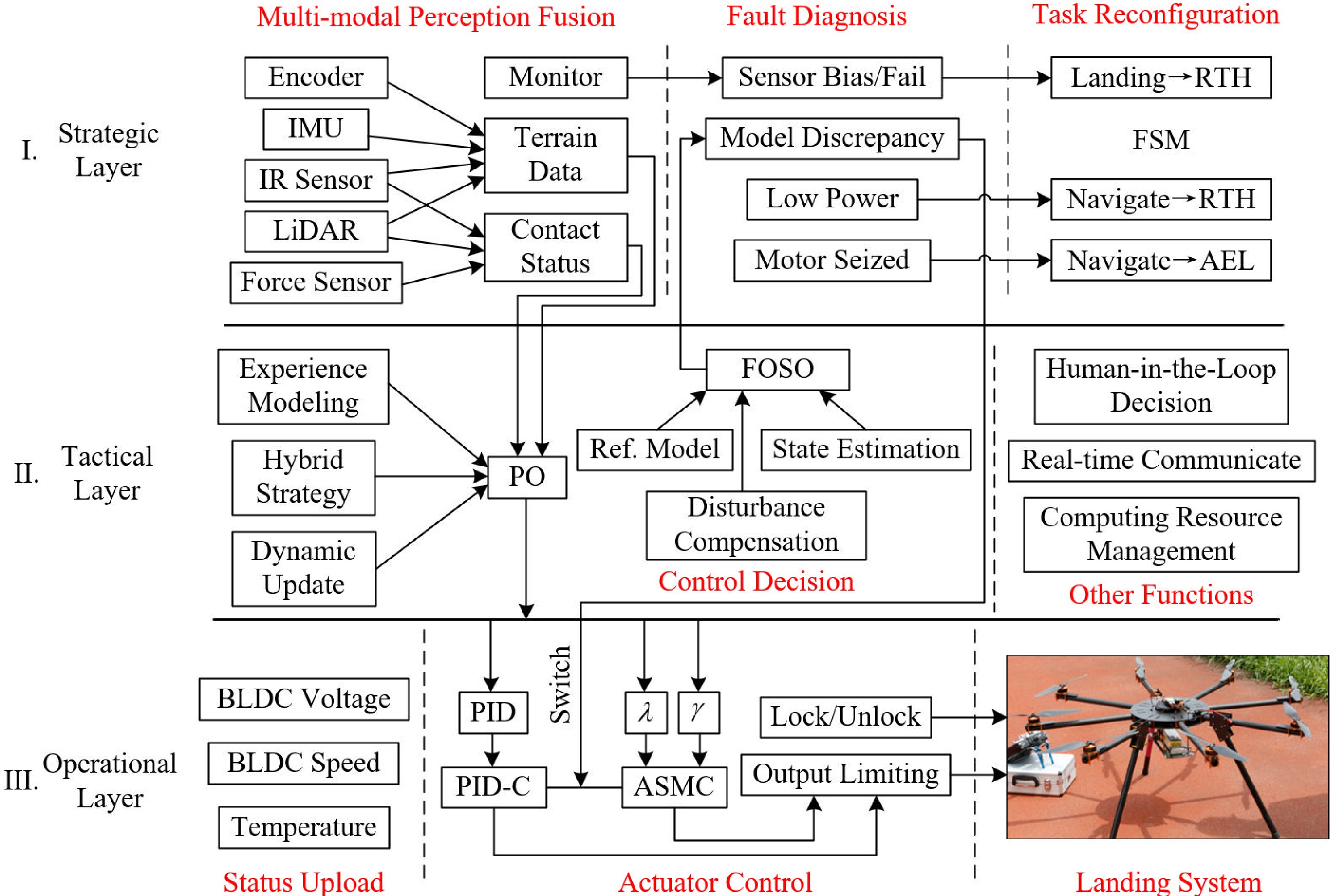
Figure 11.
Diagram of the adaptive hierarchical control framework.
-
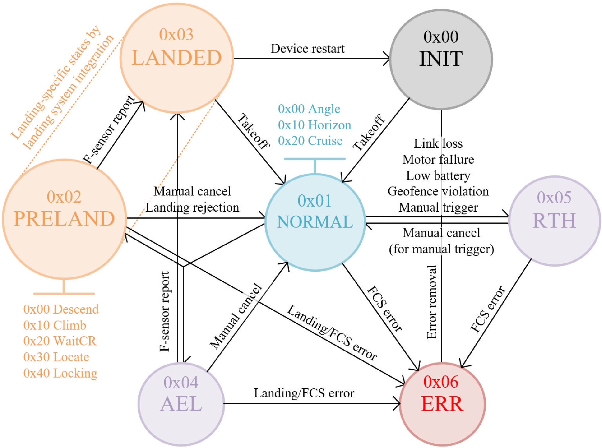
Figure 12.
Basic finite state machine framework for an intelligent multirotor UAV.
-
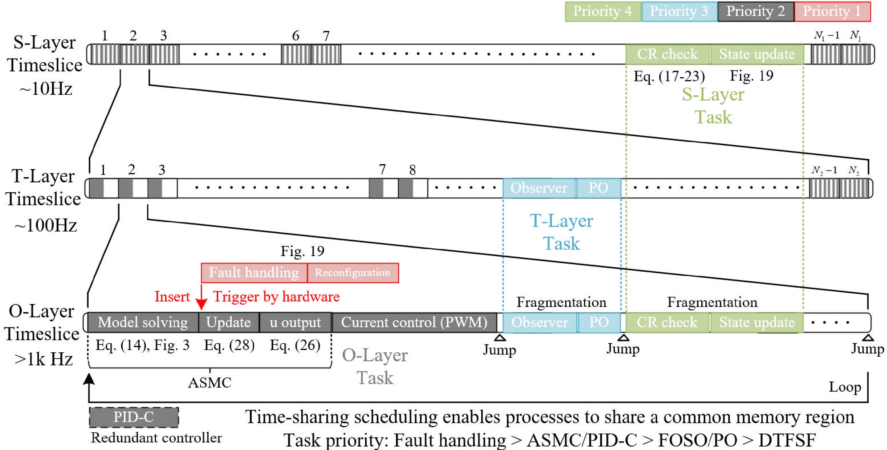
Figure 13.
Diagram of the AHCF's time synchronization with task priority.
-
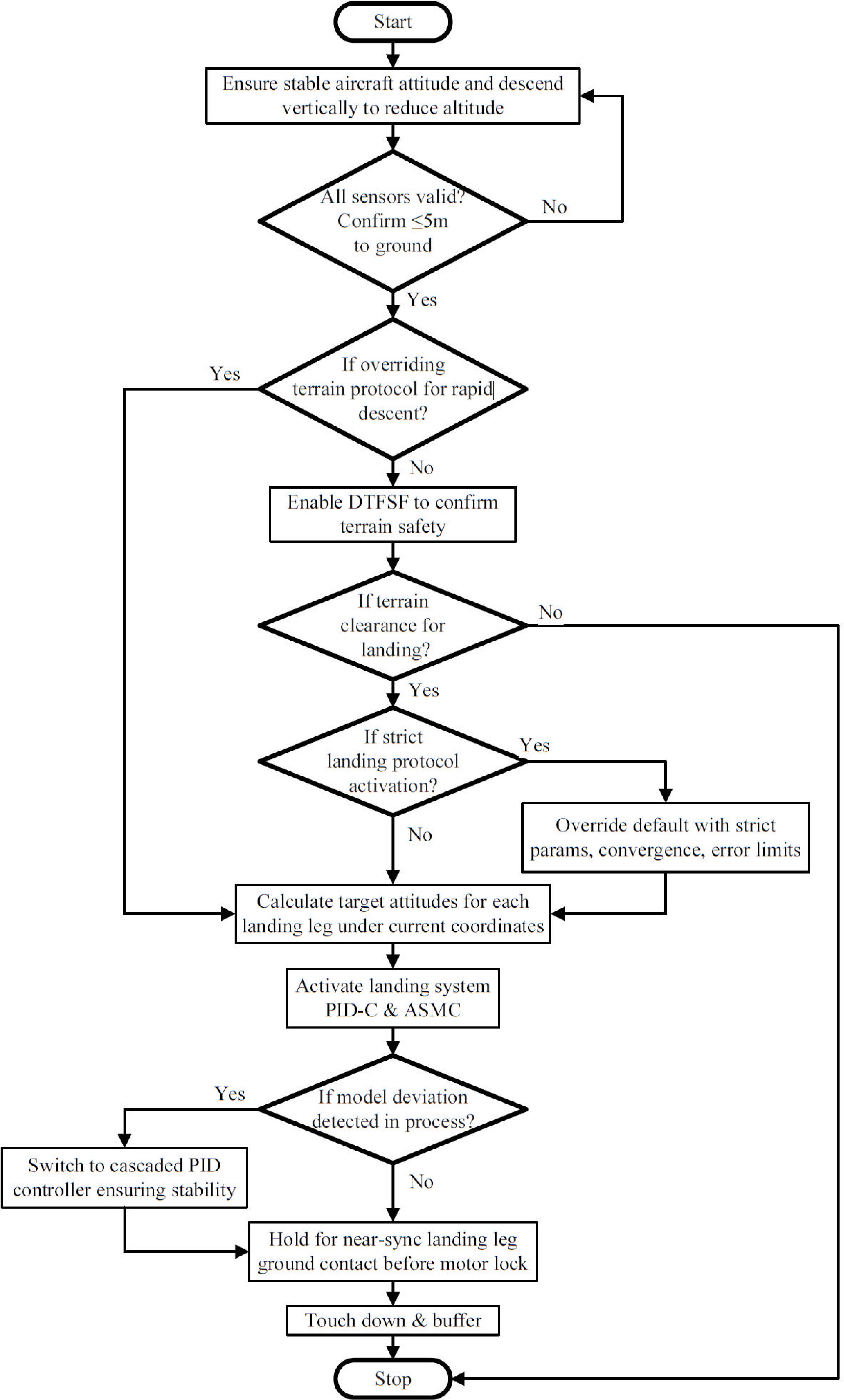
Figure 14.
Working principles and flowchart of the landing process.
-
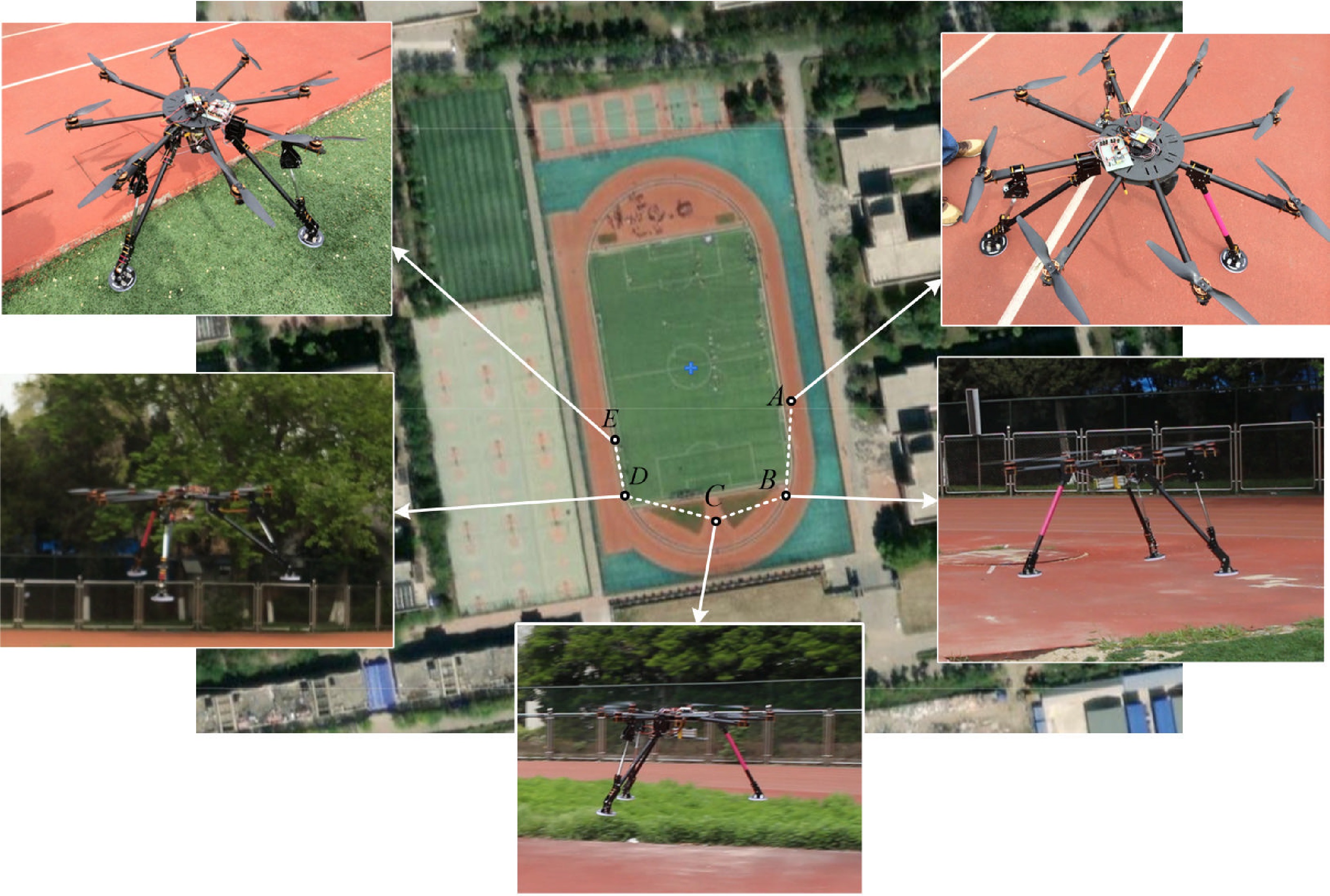
Figure 15.
Landing procedure in a real environment.
-
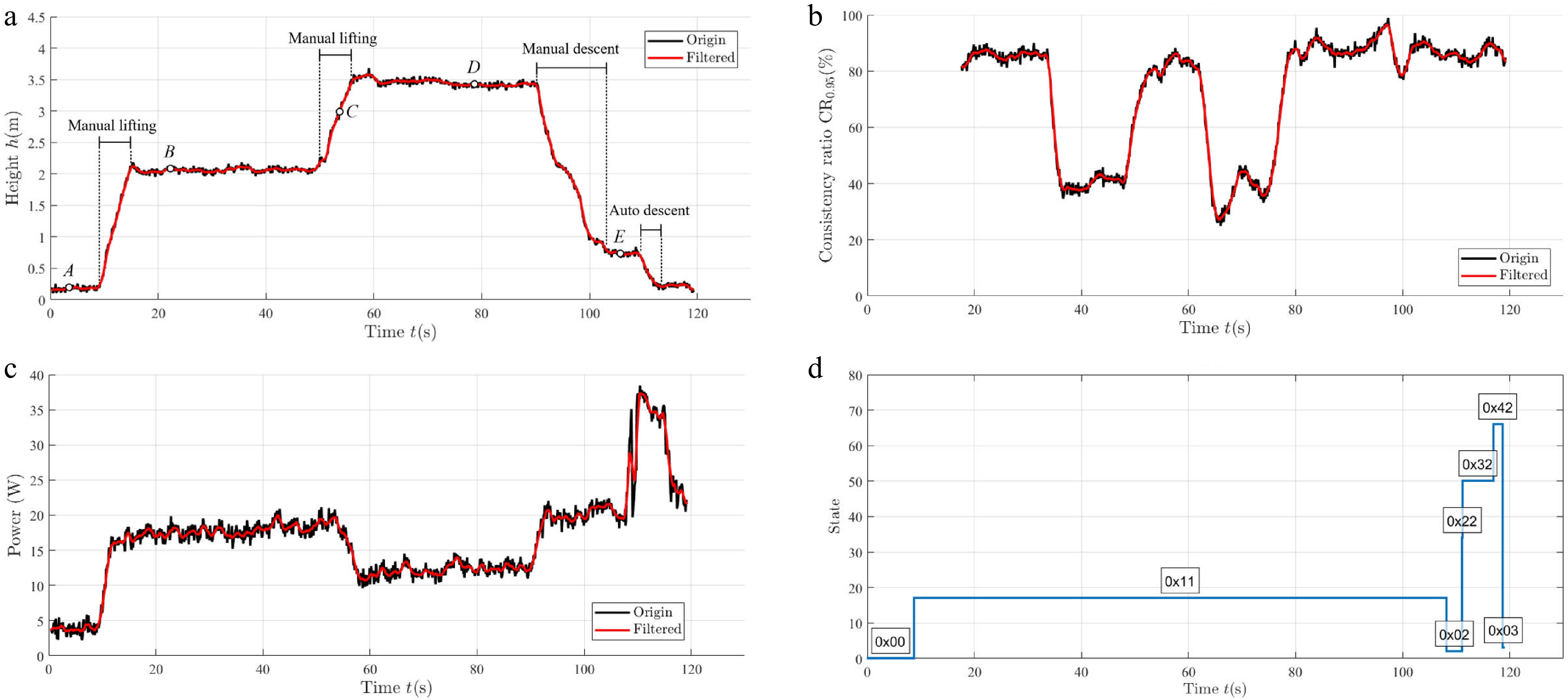
Figure 16.
Data from the entire process from INIT to LANDED. (a) Flight; (b) perception; (c) power; (d) status.
-
Terrains Landing feasibility 10 Random CR0.95 (%) Basic Flat ○ 100.00, 97.89, 96.84, 94.74, 100.00,
98.95, 100.00, 100.00, 100.00, 99.47Slope ○ 89.47, 91.05, 96.32, 82.63, 93.16,
82.11, 95.26, 94.74, 82.63, 94.74Obstacle Discrete ○ 66.84, 77.89, 55.79, 76.84, 73.68,
64.74, 60.00, 57.89, 60.53, 77.89Continuous ○ 61.58, 57.37, 71.58, 55.79, 50.53,
68.95, 55.26, 50.53, 52.11, 64.74Extreme Urban debris × 11.05, 7.37, 4.74, 5.79, 4.74, 16.84,
5.79, 10.53, 7.37, 8.42Planetary analog × 12.11, 12.68, 10.53, 12.63, 10.00,
12.11, 12.11, 9.47, 12.63, 14.21Table 1.
Quantitative evaluation of the terrains' CR.
-
Metric Full batch DTFSF Computational complexity $ \text{O}({k}^{2}) $ $ \text{O}({m}^{2}) $ Real-time performance Latency: $ {T}_{\text{delay}}=k\Delta t $ Bounded latency: $ {T}_{\text{delay}}=m\Delta t $ Memory footprint Requires storage of an $ \text{O}({k}^{2}) $ $ \text{O}(k) $ Fixed storage: $ \text{O}({m}^{2}) $ $ \text{O}(m) $ Robustness to noise Susceptible to historical noise caused by global averaging. Enhanced robustness via dynamic window updates and localized outlier rejection. Hardware compatibility Requires high-performance processors (e.g., Graphics Processing
Unit [GPU]) for large$ k $ Executable on microembedded systems (e.g., ARM
Cortex-M4) with constrained resources.Table 2.
Comparative analysis: Full batch vs. DTFSF.
-
Metric Units Proposed (1) SMC (2) PID-C (3) $ {p}_{12} $ $ {p}_{13} $ RMSE‡ 10−3 m 6.79, 0.162 8.31, 0.244 29.5, 1.52 <0.001* <0.001* IAE‡ 10−2 m·s 2.91, 0.138 3.90, 0.213 18.6, 1.94 <0.001* <0.001* ISE‡ 10−4 m2·s 4.61, 0.218 6.95, 0.380 87.2, 9.10 <0.001* <0.001* ITAE‡ 10−2 m·s2 2.89, 0.098 4.13, 0.253 42.7, 1.94 <0.001* <0.001* ITSE‡ 10−4 m2·s2 2.03, 0.0859 4.09, 0.311 76.5, 4.36 <0.001* <0.001* CE‡ 10−2 N·m·s 36.5, 1.10 35.7, 1.52 35.7, 0.917 0.998* >0.999* * Significant group difference (proposed vs. SMC and PID-C). † A battery of multiple univariate one-tailed t-tests (with Holm–Bonferroni correction) was conducted to compare the proposed controller with the two baseline controllers on all six performance indices (n = 50 trials per group, α = 0.01 with the total number of tests set to 10). ‡ RMSE is defined as $ \sqrt{\dfrac{1}{T}\int\nolimits_{0}^{T}{e}^{2}dt} $ $ \int\nolimits_{0}^{T}\left| e\right| dt $ $ \int\nolimits_{0}^{T}{e}^{2}dt $ $ \int\nolimits_{0}^{T}t\left| e\right| dt $ $ \int\nolimits_{0}^{T}t{e}^{2}dt $ $ \int\nolimits_{0}^{T}\left| {\tau }_{M}\right| dt $ Table 3.
Statistical comparison of landing performance metrics (Case 4).
-
Sensor Primary role Advantages Limitations IMU Attitude estimation High update rate, low latency Attitude drift, vibration sensitivity GPS Global positioning High accuracy, no drift, wide coverage Low update rate, signal occlusion Barometer Relative altitude Low cost, power-efficient Thermal drift, airflow disturbance IR/ultrasonic Low-altitude sensing A mm-level resolution without light Short range, rain/fog attenuation Stereo vision Terrain mapping SLAM capability, rich data High computation, lighting-dependent LiDAR Precision ranging Electromagnetic Interference (EMI)-resistant, cm-level accuracy, long range High power, rain/fog attenuation Force Detecting collisions Fast response, power efficient Affected by vibration Table 4.
Sensors potentially required for the landing phase
-
Stages Flight
MCUDTFSF Landing
MCULiDAR IR Force Cruise (>3 m) 100 MHz 10 kHz 48 MHz 5 Hz OFF OFF Near ground (<3 m) 100 MHz 10 kHz 480 MHz 10 Hz 1 kHz 1 kHz Table 5.
MCU and sensor duty cycling.
-
Modules Frequency Cycle CPU
usageOptimization Hardware
dependencyDTFSF 10 Hz 2.4 ms 2.4% CMSIS-DSP ART accelerator
+ I-cacheFOSO 100 Hz 320 μs 3.2% CMSIS-DSP FPU + DSP ASMC 1 kHz 140 μs 14% FPU-accelerated Double-precision
FPUPID-C 1 kHz 12 μs 1.2% − − Covering the key modules and the system's components. Time data were measured using Keil Microcontroller Development Kit (MDK) optimization compilation (-O3) and the on-board Discrete Wavelet Transformation (DWT) counter. Table 6.
Analysis of the core algorithm's execution time
Figures
(16)
Tables
(6)