An adaptive hierarchical control and sensor fusion strategy for an intelligent multirotor UAV landing system

The development of adaptive landing gear for rotorcraft has gained increasing interest, motivated by the demand for safer operations in dynamic environments. The initial designs concentrated on passive systems such as spring dampers, which are simple and low-cost yet cannot adjust to varying terrains. Subsequent semiactive systems, including magnetorheological dampers, improved energy dissipation but still offered limited real-time adaptability. Fully active systems using hydraulic or pneumatic actuation enabled in-flight adjustments, though they often required high energy and complex control architectures.

Internationally, research has drawn inspiration from the leg structures of birds and insects to design landing systems for unmanned aerial vehicles (UAVs) operating in complex terrain. For example, the Defense Advanced Research Projects Agency (DARPA) in the US developed a multijoint robotic leg that adjusts the leg angles in real time using tactile sensors, allowing the body to remain level on a 20° slope^[1]. However, such designs remain vulnerable to lateral impacts. Similarly, bio-inspired leg and claw mechanisms have been developed at Stanford University^[2], Skolkovo Institute^[3], the University of Tokyo^[4], Eidgenössische Technische Hochschule (ETH) Zurich^[5], and the University of Edinburgh's Napier University^[6]. A recurring limitation across these systems is their structural vulnerability under lateral forces. Integrating buffering components could help distribute the impact loads, but current research has not sufficiently addressed the dynamic interaction between the landing mechanisms and complex terrains. Most systems have been validated only on flat surfaces, limiting their applicability in unstructured environments.

Multisensor fusion has become a key enabler for improving reliability and environmental adaptability^[7]. The related research approaches fall into three main categories: Deep learning-based feature fusion, adaptive fault-tolerant control^[8], and real-time processing techniques.

In deep learning-driven fusion, efforts focus on integrating multimodal data and advanced feature extraction. Yang et al.^[9] introduced a local–global fusion architecture using sparse transformers to handle limited training samples. Xu et al.^[10] combined Principal Component Analysis (PCA)-based sensor fusion with spiking neural networks. Parsons et al.^[11] designed a dual-channel convolutional neural network (CNN) for light detection and ranging (LiDAR), and red–green–blue (RGB) data, improving object detection robustness. Lv et al.^[12] proposed a hierarchical residual long short-term memory (LSTM) with dynamic attention. Though such neural network methods capture intricate data patterns, their computational demands often hinder real-time performance in UAV landing applications.

In fault-tolerant control, Sun et al.^[13] developed an adaptive tracking control framework using historical data-driven weighting to counteract sensor faults and disturbances. Wu et al.^[14] integrated adaptive control with sensor fusion in a variable-weight Model Predictive Control (MPC) structure. However, many methods treat sensor errors as disturbances and may fail if the controller becomes unstable, highlighting the need for modular designs.

For real-time processing, researchers have emphasized computational efficiency and noise suppression. Hussain et al.^[15] compared fusion methods for space target tracking, showing a balance between accuracy and speed. Wang et al.^[16] proposed a distributed multirate fusion algorithm using sequential Weighted Minimum Mean Square Error (WMMSE) estimation to handle unknown noise correlations. Xu et al.^[17] incorporated state saturation and the sensors' resolution into a covariance intersection framework. These optimization methods perform well with limited data and improve systems' efficiency.

Recent perception-driven landing strategies combine vision, LiDAR, and Inertial Measurement Unit (IMU) data to improve landing precision. Ban et al.^[18] fused camera, LiDAR, and IMU data with green feature mapping and point cloud fusion. Sestras et al.^[19] integrated LiDAR and photogrammetric data for robust terrain modeling. Liu et al.^[20] developed a semantic Simultaneous Localization and Mapping (SLAM) framework with object-level clustering. Saldiran et al.^[21] created a LiDAR-based grid-processing system for emergency landings under critical failures. Chen et al.^[22] implemented multisensor SLAM for parafoil UAVs in complex terrains. Jiao et al.^[23] achieved real-time centimeter-accurate semantic mapping via LiDAR–visual–inertial fusion. Despite these advances, such methods lack the adaptive hierarchical control needed to balance the computational load and precision across dynamic landing scenarios.

For rotorcraft landing systems requiring high tracking accuracy and speed, linear control methods^[24] may be inadequate. Sliding mode control (SMC) has gained attention, as it combines the simplicity of proportional–integral–derivative (PID) control with bounded error and exponential convergence. SMC drives a system's states to a predefined sliding surface in finite time and offers robustness against disturbances and parameter variations.

Although SMC for linear systems has been widelystudied^[25,26], its application to nonlinear systems like rotorcrafts' landing gear remains challenging, mainly because of chattering—high-frequency oscillations caused by discontinuous control actions. Recent studies have proposed techniques for mitigating chattering. Labbadi et al.^[27] applied backstepping to derive error dynamics and designed switching laws to suppress chattering^[28,29]. Irfan et al.^[30] developed chattering-free SMC for a twin-rotor UAV. Robust SMC schemes can handle complex nonlinear dynamics^[31], and saturation-constrained SMC is suitable for mechanical systems^[32]. A fast integral terminal SMC has also been proposed for robotic systems^[33]. Though innovative, such methods still lack the speed and reliability needed for landing systems' decision-making.

In summary, a significant research gap persists in unifying robust mechanical designs, real-time perception, and adaptive control into a cohesive system capable of handling uncertainties in complex landing scenarios. To address this, the present study introduces the following:

(1) A bio-inspired linkage-based landing mechanism with a tri-leg configuration that simplifies control, ensures redundancy, and favors axial loading for improved terrain adaptation;

(2) A sliding-window terrain perception algorithm, known as the dynamic terrain flatness scanning and fusion (DTFSF) model, using LiDAR/infrared sensors and IMU for real-time, noise-resistant terrain identification on embedded platforms;

(3) A Lyapunov-stabilized adaptive sliding mode controller (ASMC) robust to model the uncertainties, partial actuator failures, and external disturbances;

(4) An adaptive hierarchical control framework (AHCF) that integrates mechanical, perception, and control layers to enable autonomous landing in complex environments.

In large aircraft, the landing gear is categorized into three types depending on the shock absorbers' position and the load-bearing mode: Strut-type, semilevered, and levered. In levered landing gear, the shock absorber withstands axial forces only. This configuration enhances the resistance to forward impact loads, improves ground taxiing stability, reduces bushing friction, decreases wear, and improves the sealing performance. However, it is relatively heavy and requires more space for retraction.

Considering the trade-off between weight and flexibility, we developed a rocker-actuated adaptive landing gear for an octocopter UAV (Fig. 1). Inspired by levered landing gear, a servo-driven lead screw actuator adjusts the landing legs' angle. The drive mechanism withstands axial forces only and forms a stable triangular configuration with the airframe and landing legs. A single landing leg can be simplified into a planar two-bar constrained structure, with only one constraint equation (Eq. [1]), thus resulting in one degree of freedom (DoF).

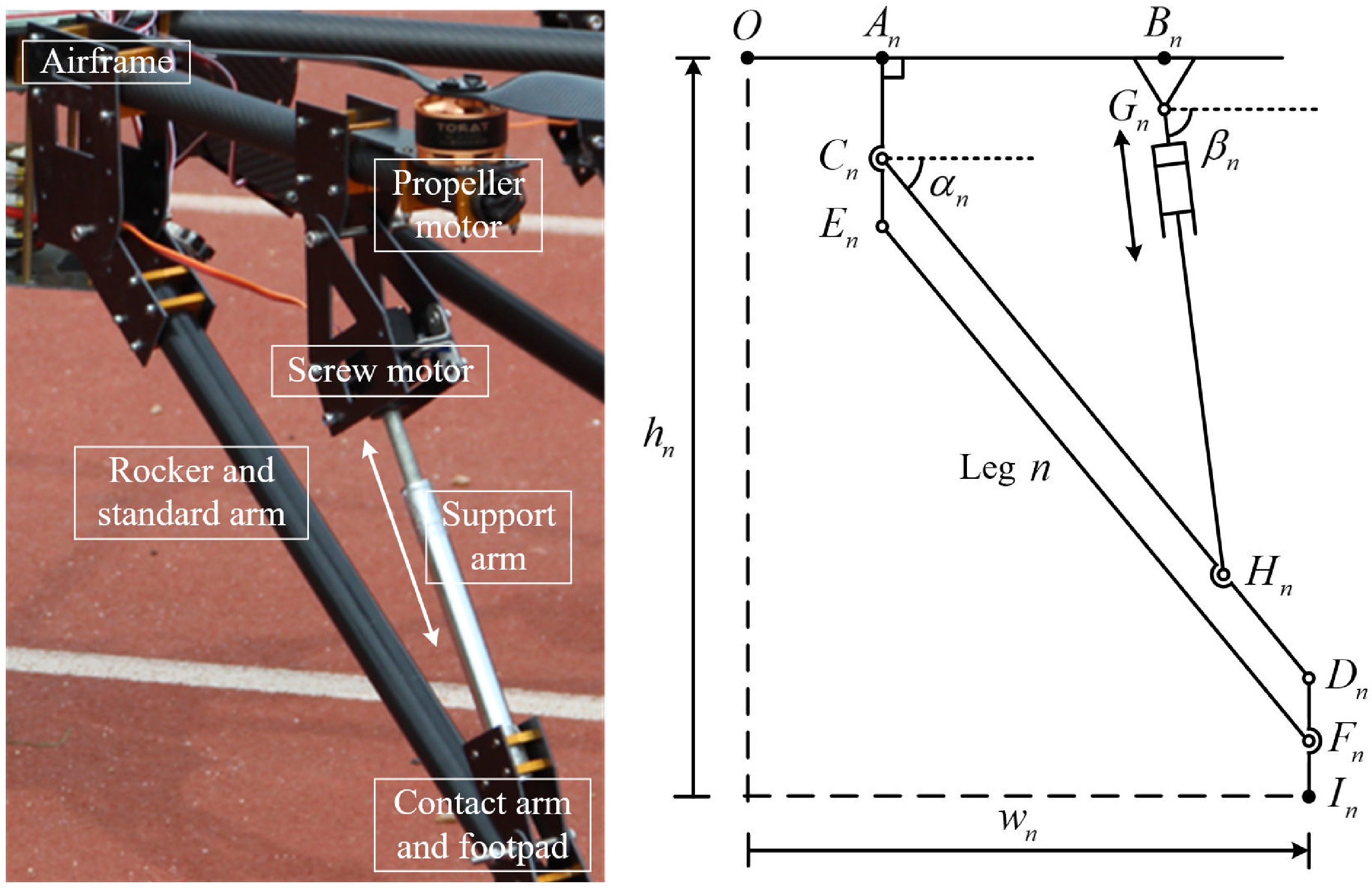
Figure 1. 

Single rocker-actuated landing leg.

The entire landing system consists of two rocker-actuated landing leg and one fixed landing leg (see Fig. 2), arranged in a triangular formation when viewed from the vertical direction. This configuration ensures that the system contacts the ground at three different heights, allowing the rotorcraft to achieve a stable landing on certain complex terrains. Under these conditions, the number of control variables in the system is reduced to two, thereby minimizing the weight of the motors and increasing the payload capacity of the rotorcraft. The system exhibits high flexibility, as the fixed landing leg can be removed, leaving three rocker-actuated landing legs. This ensures that the system can still land on complex terrains even if one leg fails, providing robustness.

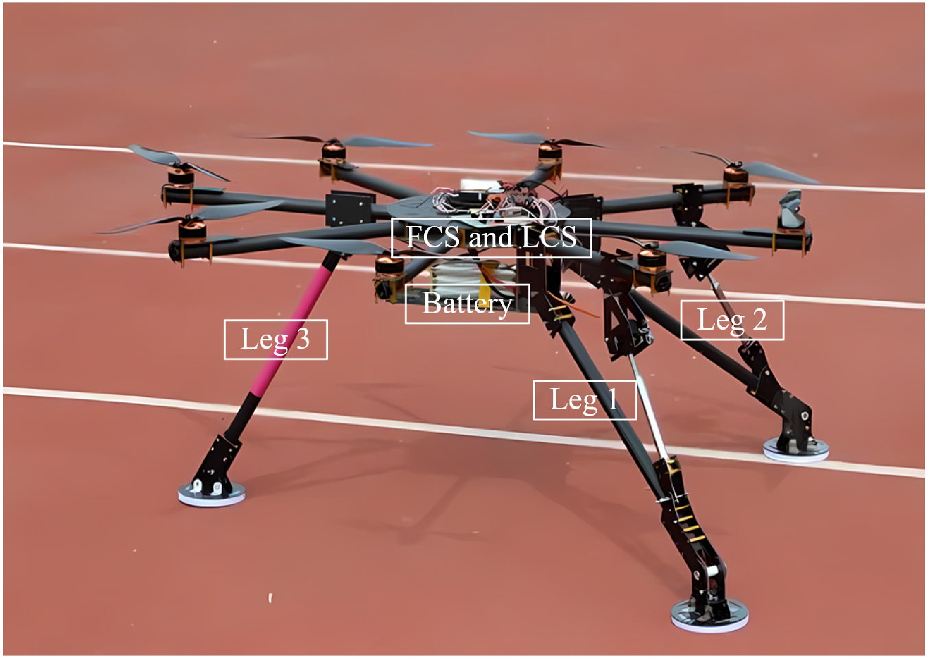
Figure 2. 

Movable legs (Nos. 1−2, black) and fixed leg (No. 3, red).

Based on the mechanism schematic shown in Fig. 1, the kinematic equations (Eqs. [1]−[4]) relating the motor's rotation to the terminal horizontal/vertical motion of the rocker-actuated landing leg can be derived. The angles α_n, β_n represent the angles between the rocker arm C_nD_n and the support arm G_nH_n, respectively, and the drone's horizontal plane. The distances w_n, h_n denote the width and height of the landing leg tip, measured with respect to the drone's center axis as the zero point. L with a subscript represents the length of the arm.

Here, n = 1, 2 denotes the index of the movable landing leg. The support arm is designed with a right-handed thread. In this configuration, the elongation of the support arm is determined by the rotation angle of the motor r(t) (in radians) and the pitch p, satisfying Eq. (5). When viewed from above the drone, the rotation is defined as positive when the motor turns counterclockwise.

When the mechanical structure changes over time, the velocity kinematics equation for a landing leg system is given by Eqs. (6) and (7). The single-motor actuation scheme inherently induces a coupling relationship between the terminal horizontal dw_n and vertical velocities dh_n.

Dynamic modeling

To facilitate the derivation of the dynamic model while preserving the fundamental characteristics of the system, the following standard assumptions are adopted:

(1) Rigid body assumption: All components are rigid; elastic deformations are neglected.

(2) Lumped parameter model: The system's properties (mass, damping, stiffness) are concentrated at discrete points.

(3) Ideal joints: The joints are frictionless, without backlash or hysteresis.

(4) Idealized actuators: The actuators are perfect sources of torque or force sources; the internal dynamics are neglected.

(5) Uniform gravity: A constant gravitational field is assumed for consistent potential energy reference.

These assumptions yield a deterministic, time-invariant, nonlinear model, forming the basis for the controller's design and stability analysis. Though it is simplified, it captures the dominant dynamics that are essential for evaluating this work's core contributions.

The landing leg's dynamic model is derived using Lagrangian mechanics, a framework that is ideal for constrained systems with multiple degrees of freedom. This energy-based approach enables a systematic derivation of the equations of motion, simplifying the analysis of complex systems like the landing leg by avoiding direct force calculations.

The length of the arm G_nH_n, as the variable s_n, is selected as the independent coordinate to compute the kinetic and potential energy of the entire landing leg. The dynamics of a landing leg are primarily constituted by the following four active linkages: the rocker arm C_nD_n, the standard arm E_nF_n, the support arm G_nH_n, and the contact rod D_nI_n. The kinetic energy K_n, the potential energy P_n, the generalized forces, and the Lagrange equation of a single landing leg are described in Eqs. (8)−(11), where m with an arm's name as the subscript represents the mass of the arm.

The dynamic parameter with s_n, $ {\dot{s}}_{n} $ as the variables is denoted M_n, C_n, G_n. The Lagrangian equation for the n-th landing leg simplifies to:

By substituting the independent variable s_n with h_n and updating the dynamic parameters to $ {{{M}^{\prime}}}_{n},\;{{{C}^{\prime}}}_{n},\;{{{G}^{\prime}}}_{n} $, the dynamic equation of height (Eq. [13]) for a single landing leg is derived. Subsequently, by synthesizing the dynamics of both landing legs, the multibody dynamic equation (Eq. [14]) for the landing system is obtained.

where, $ {M}_{L}\in {\mathbb{R}}^{n\times n} $ is the mass matrix, $ {C}_{L}\in {\mathbb{R}}^{n\times n} $ contains the Coriolis and centrifugal terms, and $ {G}_{L}\in {\mathbb{R}}^{n} $ is the gravity vector, which incorporates the inertia and gravitational effects of the entire landing system. Under low-speed operation of the landing legs, the influence of higher-order terms (unmodeled dynamics) of State $ \mathbf{H } $ on the system is negligible. The conservative and nonconservative forces within the system originate from the motor's actuation, ground contact, and joint–motor friction.

According to the static analysis, the support arm bears the primary compressive force. Because of the unique characteristics of the lead screw transmission, the angle of the compressive force acting on the screw thread exceeds the friction angle of the contact surface, resulting in a self-locking phenomenon. This indicates that the energy cannot propagate into the system, and thus its impact is disregarded until full landing is achieved. The combined friction is aggregated into a single term and operates in the same channel as the motor control input.

A model for the dynamic perception of landing

To enhance the model's accuracy, the landing system's potential energy is dynamically adjusted on the basis of the aircraft's six-axis attitude (Figs. 3, 4). The method involves the following.

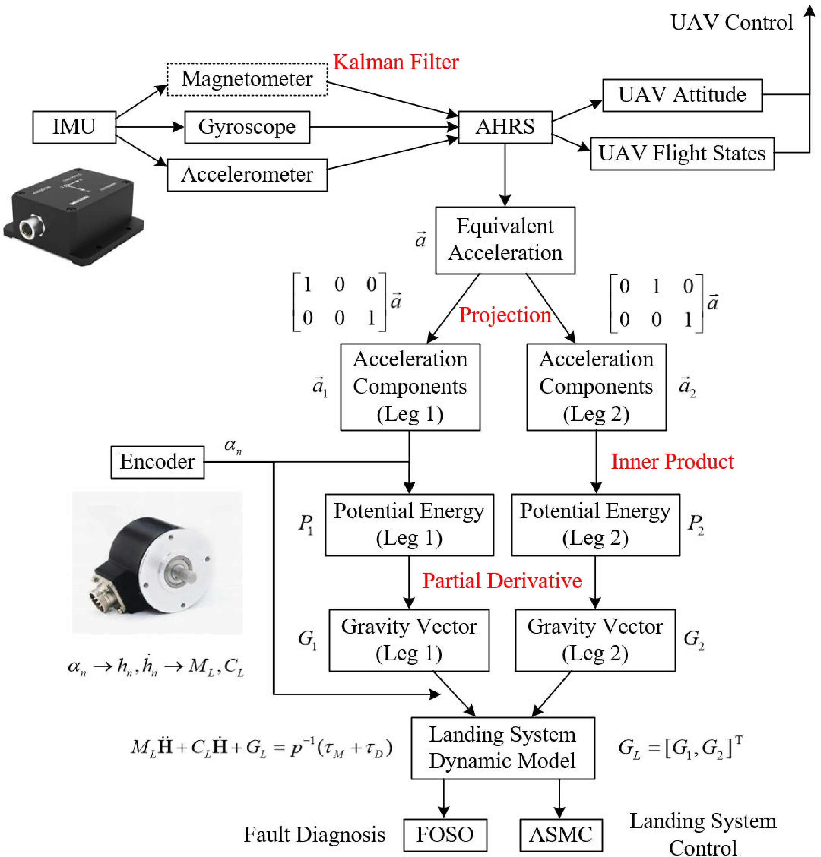
Figure 3. 

Dynamic model solution for the landing system.

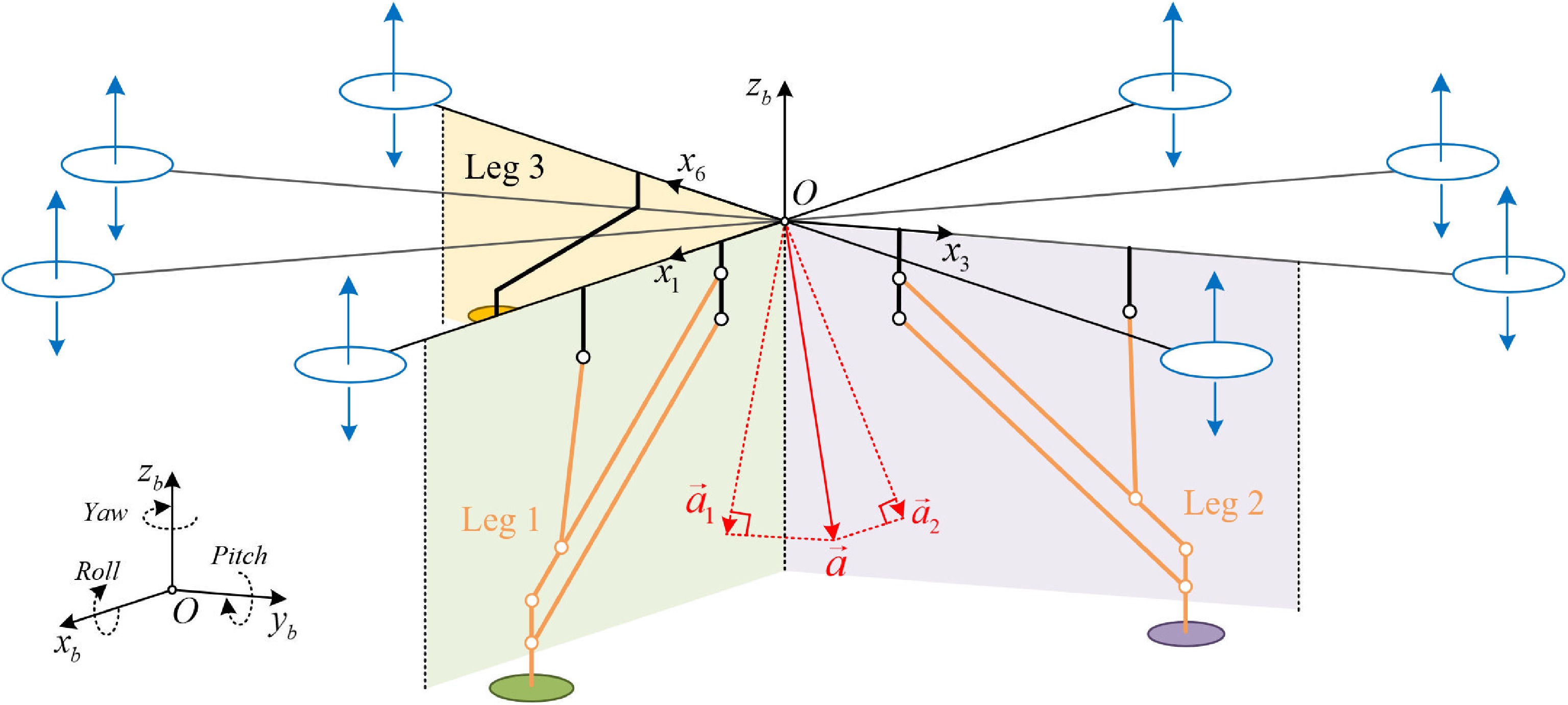
Figure 4. 

Dynamic perception strategy for the landing model.

Acquisition of the gravity vector: The equivalent gravity in the inertial frame is obtained from accelerometers or an attitude and heading reference system (AHRS) by extracting the low-frequency gravitational component.

Transformation and projection of the coordinates: Gravity is transformed to the airframe and projected onto two orthogonal planes ($ O{x}_{1}z,O{x}_{3}z $) to get the components $ {\overrightarrow{a}}_{1} $ and $ {\overrightarrow{a}}_{2} $. A leg extension angle is acquired via an encoder.

Calculation of potential energy: Taking the UAV's center O as the zero point, the leg's potential energy is computed by summing the inner products of the gravity components and linkage vectors in their respective planes.

According to Eq. (13), the system's matrices M_L, C_L, and G_L and are nonlinear functions of the leg's height or velocity. Real-time parameter updates make the dynamic model converge toward the actual physics. This refined model drives the ASMC controller and initializes the full-order state observer (FOSO). The observer runs in parallel, providing states for verifying the ASMC's stability.

This model reveals that the two legs, though driven independently, exhibit low coupling because of the numerical correlations between the gravity components. Thus, they can be treated as decoupled, independent systems. Distributed parallel computing via Microprocessor Unit (MPU) communication halves the computation time while maintaining precision.

The DTFSF algorithm uses data from at least four ranging sensors and one attitude sensor to perform terrain detection, classification, and error correction during low-altitude UAV flight. It incorporates a sliding window mechanism to ensure the data's timeliness and efficient Microcontroller Unit (MCU) memory use, enabling intelligent landing on compact embedded devices (the process is shown in Fig. 5).

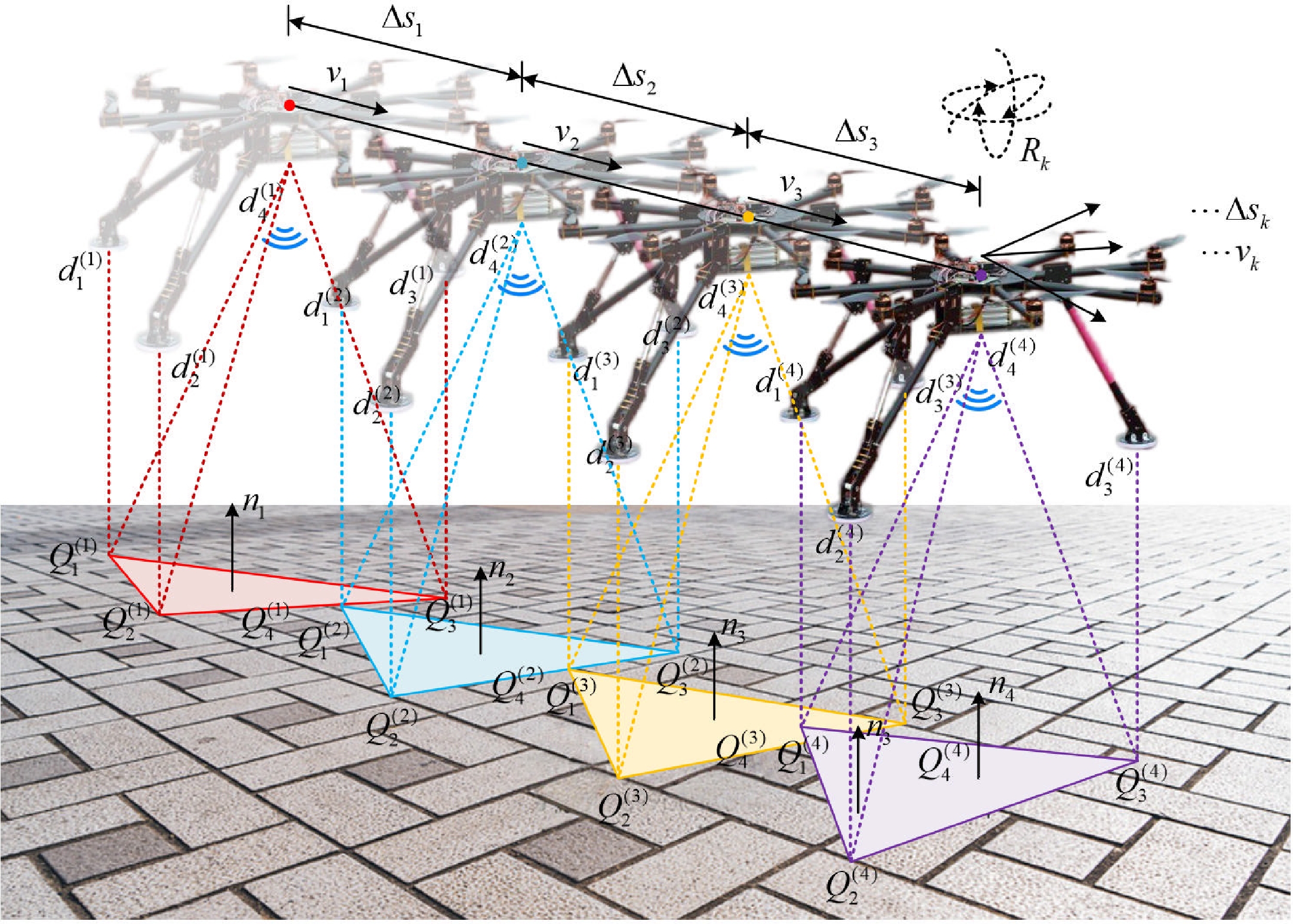
Figure 5. 

Schematic diagram of the DTFSF method.

Although the current ranging sensors operate at 300−1,000 Hz, traditional point cloud processing methods are too computationally expensive for small embedded systems. DTFSF overcomes this by replacing complex classifiers with optimized geometric primitives, achieving real-time terrain assessment in just 1 ms on microcontrollers like the STM32H7 (50× faster than PCA). It maintains high recognition accuracy for typical terrains with minimal data. Crucially, for landing, UAVs only need to detect local flatness within the landing zone, not map the entire area, enabling a rapid touchdown.

Step 1. The system's setup

Three ranging sensors are mounted on the three legs' endpoints and on one LiDAR system at the airframe center. Let the positions of sensors in the airframe be $ {P}_{1},{P}_{2},{P}_{3}\in {\mathbb{R}}^{3} $ (mounted on the three legs) and $ {P}_{0}\in {\mathbb{R}}^{3} $ (the center of the airframe). $ {P}_{i} $ is determined from the installation position of the landing leg and the kinematic equation, that is:

To ensure full coverage of all landing legs by the center LiDAR's point cloud prior to touchdown, the vertical field of view (FOV) $ {\theta }_{v} $ must satisfy the following:

where, s_min denotes the minimum permissible length of the support strut.

Step 2. IMU-based ground point acquisition

At each movement step t < k, the UAV moves by $ \Delta {s}_{t} $ along a direction v_t. The ground contact points are directly computed in the airframe as follows:

where, $ {\hat{z}}_{b}={(0,0,1)}^{ \text{T}} $ is the vertical unit vector of the airframe, $ d_{i}^{(t)} $ represents the filtered ranging result of the i-th infrared (IR) sensor of step $ t $, $ {R}_{t}\in {\mathbb{R}}^{3\times 3} $ is the roll–pitch–yaw (RPY) rotation matrix of the rotor UAV's airframe at the current position relative to the initial point (t = 0).

Note: Certain LiDAR models directly output relative coordinates, enabling one to bypass the coordinate transformation steps.

Step 3. Sliding window initialization

Define a sliding window covering the latest $ m $ movement steps as follows:

Step 4. LiDAR–ranging sensor fusion

Fault detection leverages hardware redundancy and a statistical consistency check (a two-sample t-test) between the measurements of LiDAR and the ranging sensor over the sliding window. If significant inconsistency is detected for a single leg, that ranging sensor's confidence is downweighted. If inconsistencies occur on two or more legs, the LiDAR's confidence is downweighted instead.

Step 5. Local and global normal vector

For each $ t\in {W}_{k} $, compute the plane normal vector using three noncollinear points as follows:

Construct the normal vector matrix $ {\mathbf{N}}_{W} $ for the window as follows:

Compute the following cosine similarity matrix (CSM) $ {\mathbf{S}}_{W}\in {\mathbb{R}}^{m\times m} $:

Step 6. Dynamic flatness decision

Define the thresholds λ (angular tolerance) and κ₁, κ₂ (0 < κ₂ < κ₁ < 1) (consistency ratio). Here, $ {\mathbf{S}}_{u,v} $ is the element in the u-th row and v-th column of the matrix $ {\mathbf{S}}_{W} $, where 1 ≤ u, v ≤ m. The landing mode will be changed to "strict" if

where, $ {\mathbb{I}}_{\{*\}} $ is a logical operator that outputs 1 when the statement * in the brace is true, and 0 otherwise. The intelligent landing control system (LCS) will reject the landing command if

This indicates that CR_λ serves as a critical indicator reflecting the terrain's flatness.

Figure 6 presents a flowchart summarizing Steps 1 to 6. To ensure that each displacement vector generates useful ground information, the direction v_t and distance Δs_t are determined by the rotorcraft's path planning algorithm (boustrophedon, genetic algorithm [GA] or particle swarm optimization [PSO]), such that all sampling points are uniformly distributed within the prelanding area. The size of this area is typically determined by the horizontal dimensions of the UAV, and it is generally set to 3−5 times the UAV's size.

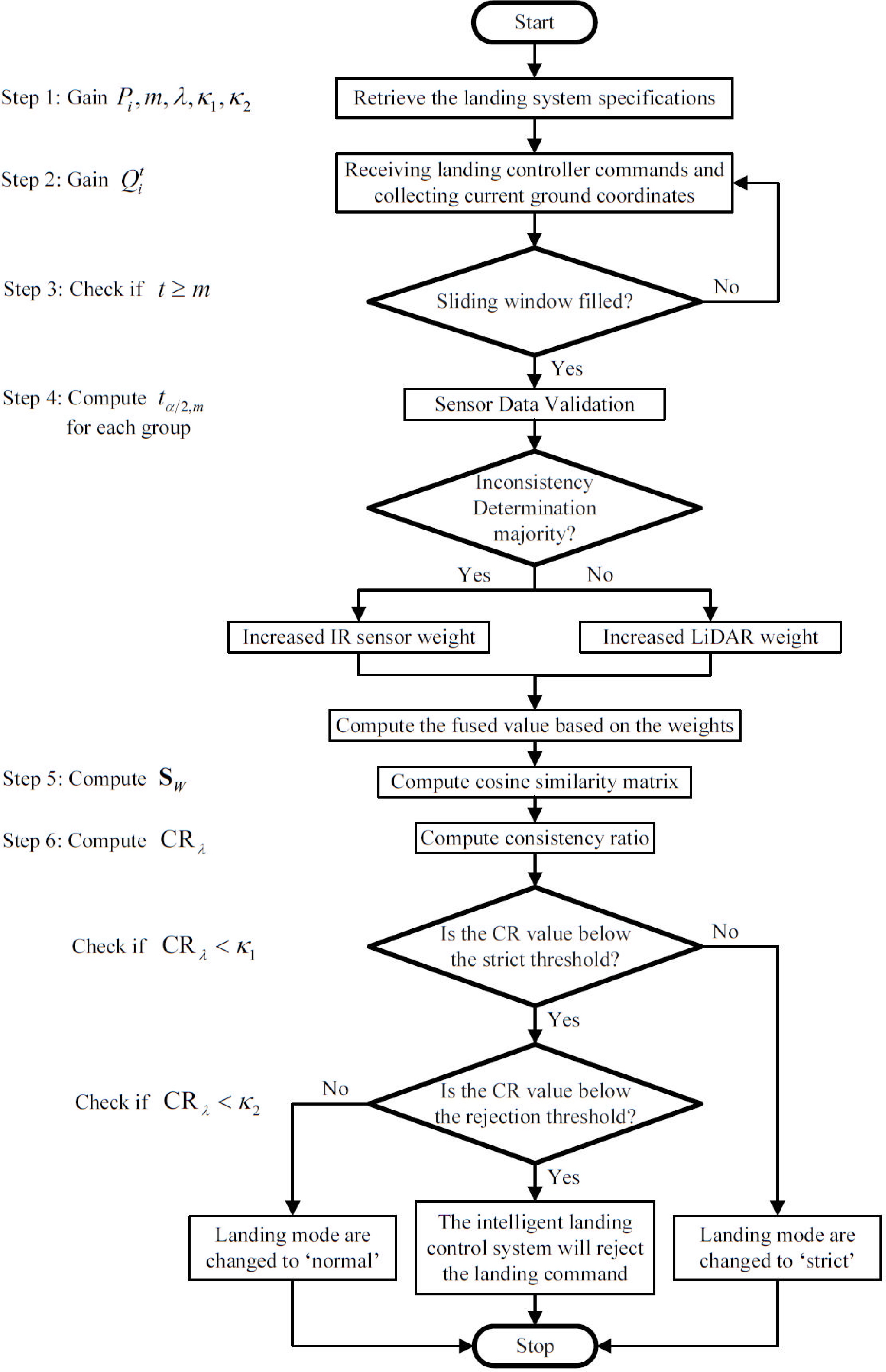
Figure 6. 

Flowchart of the DTFSF method.

Multiterrain simulation

To validate the effectiveness of the algorithm, we utilized real terrain data to compute the CR_0.95. The terrains included basic terrains (flat and slope), obstacle terrains (rocks, trenches, and staircases), and extreme terrains (urban debris or planetary analogs) to ensure diversity. For the aforementioned terrains, a dedicated terrain model was implemented in for simulations with the DTFSF algorithm. Paths were generated with complete randomness at step sizes below the maximum leg span (0.5–0.8 m in this study) to ensure full coverage of all triangular facets. The sliding window width was empirically set to 20. Gaussian functions (μ = 0, σ = 0.02 m = measurement accuracy) modeled potential ranging sensor errors. Each terrain underwent 10 randomized path simulations, with representative paths visualized in Fig. 7. The black lines depict the trajectories of the UAV's center, the red points indicate ground projections of the ranging sensors (approximating the measurement locations), and the blue-shaded regions represent convex hulls encompassing all measurement points.

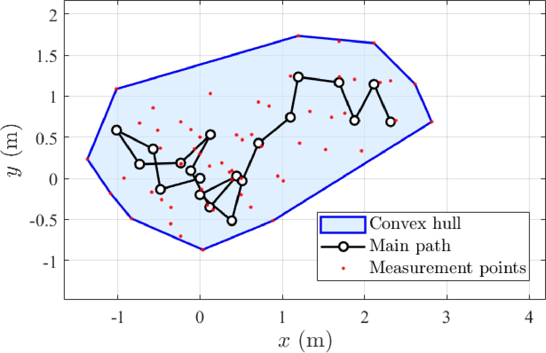
Figure 7. 

Illustration of a randomized path (m = 20).

The visualization of the landing terrain's CSM is shown in Fig. 8. The performance metrics are quantified in Table 1.

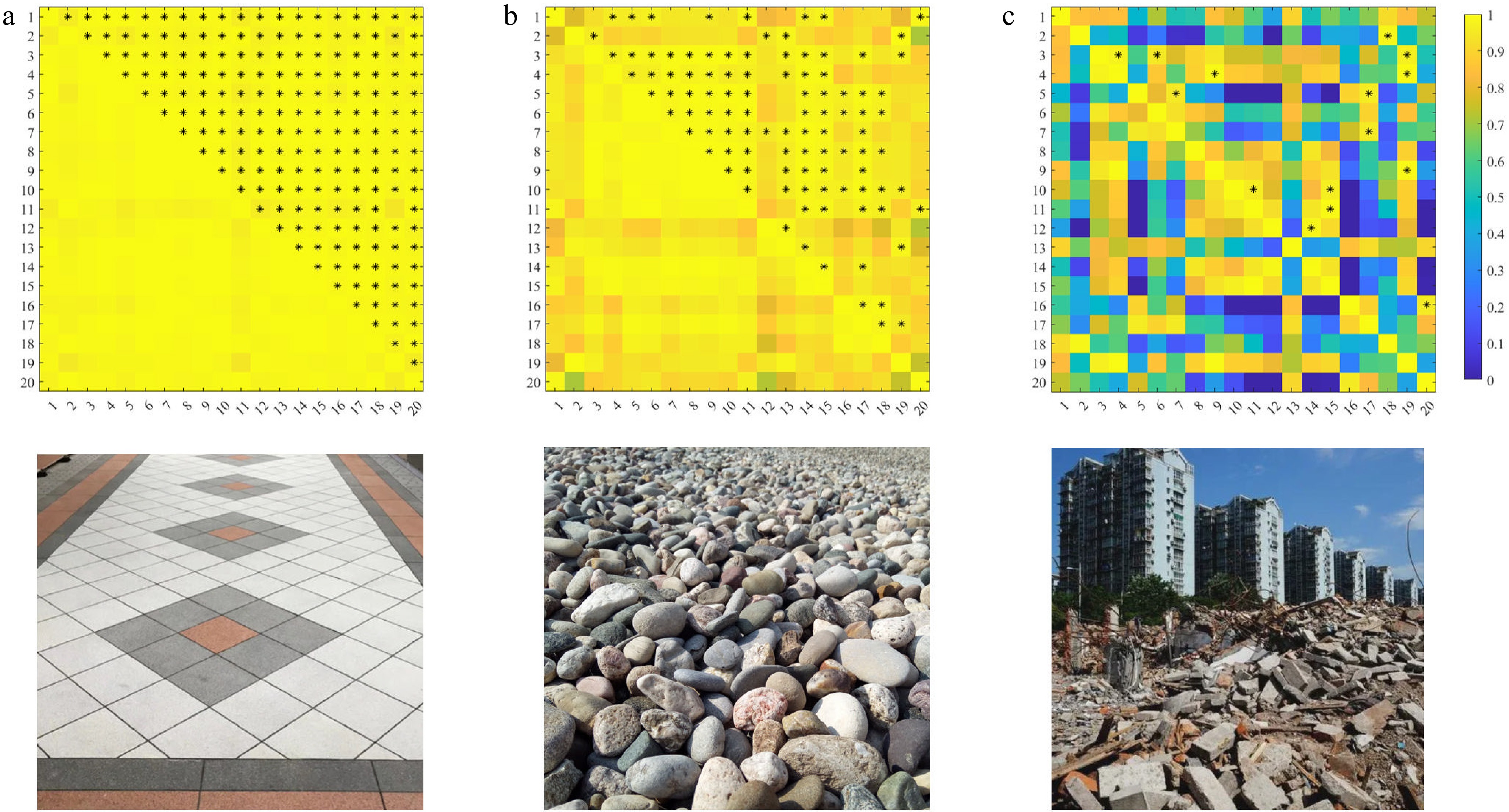
Figure 8. 

Landing terrain types and the corresponding CSM: (a) Basic, (b) obstacle, and (c) extreme.

As one can see in Table 1, the experimental results demonstrate a statistically significant correlation between the terrain's complexity and the CR_0.95 metric, validating the efficacy of the DTFSF algorithm in dynamic terrain assessment. Flat terrain exhibited near-optimal CR_0.95 values (mean: 98.7%, range: 95%–100%), indicating minimal terrain-induced risks and suitability for autonomous landing. In contrast, sloped terrain showed moderate degradation (mean: 90.2%, range: 82%–96%), necessitating adaptive control strategies to mitigate slope-induced uncertainties. Obstacle terrains, particularly continuous obstacles (mean: 58.8%, range: 51%–72%) and extreme terrains, including urban debris (mean: 8.3%, range: 4%–17%) and planetary analog terrains (mean: 11.8%, range: 9%–14%), exhibited near-zero CR_0.95 values, aligning with their inherent structural irregularities and reinforcing the necessity of preemptive landing cancellation. Our simulation results across diverse terrains (Table 1) demonstrate that CR_0.95 effectively distinguishes optimally flat terrain, slopes, and obstructed terrains, providing a robust safety margin while maintaining practical applicability. The hierarchical CR_0.95 thresholds (> 80%: safe; 50%–80%: strict; < 50%: reject; i.e. κ₁ = 0.8, κ₂ = 0.5), effectively operationalize terrain-driven decision-making, underscoring the algorithm's robustness in diverse real-world scenarios.

The selection of specific λ thresholds for high-confidence safe landing was determined through an extensive empirical analysis of the trade-off between the ability to discriminate the terrain and operational safety. A higher threshold would excessively restrict landing opportunities on undulating yet safe terrains, leading to unnecessarily aborted landings and reducin the system's utility. Conversely, a lower threshold would compromise the acquisition of terrain information within the sliding window and increase the risk of accepting areas with potential localized hazards, thereby affecting the landing's stability.

Analysis and comparison of the DTFSF algorithm

In the DTFSF algorithm, both the step size and sliding window width critically influence the terrain assessment metrics. Intuitively, smaller step sizes and wider windows increase the measurement density within local regions, theoretically improving the accuracy of the analyses. We sampled 120 datasets (20 per terrain type across six terrains). For window sizes {1, 5, 10, 20, 30, 50}, each dataset's CR_0.95 output was classified into three terrain types: Extreme (0%−50%), obstacle (50%−80%), and basic (80%−100%).

Four sampling strategies were implemented:

(1) Variable step: inversely proportional to the gradient;

(2) Fixed step: Below the sensors' spacing, approximately equal to the sensors' spacing, or exceeding the sensors' spacing.

The results of classification accuracy are shown in Fig. 9.

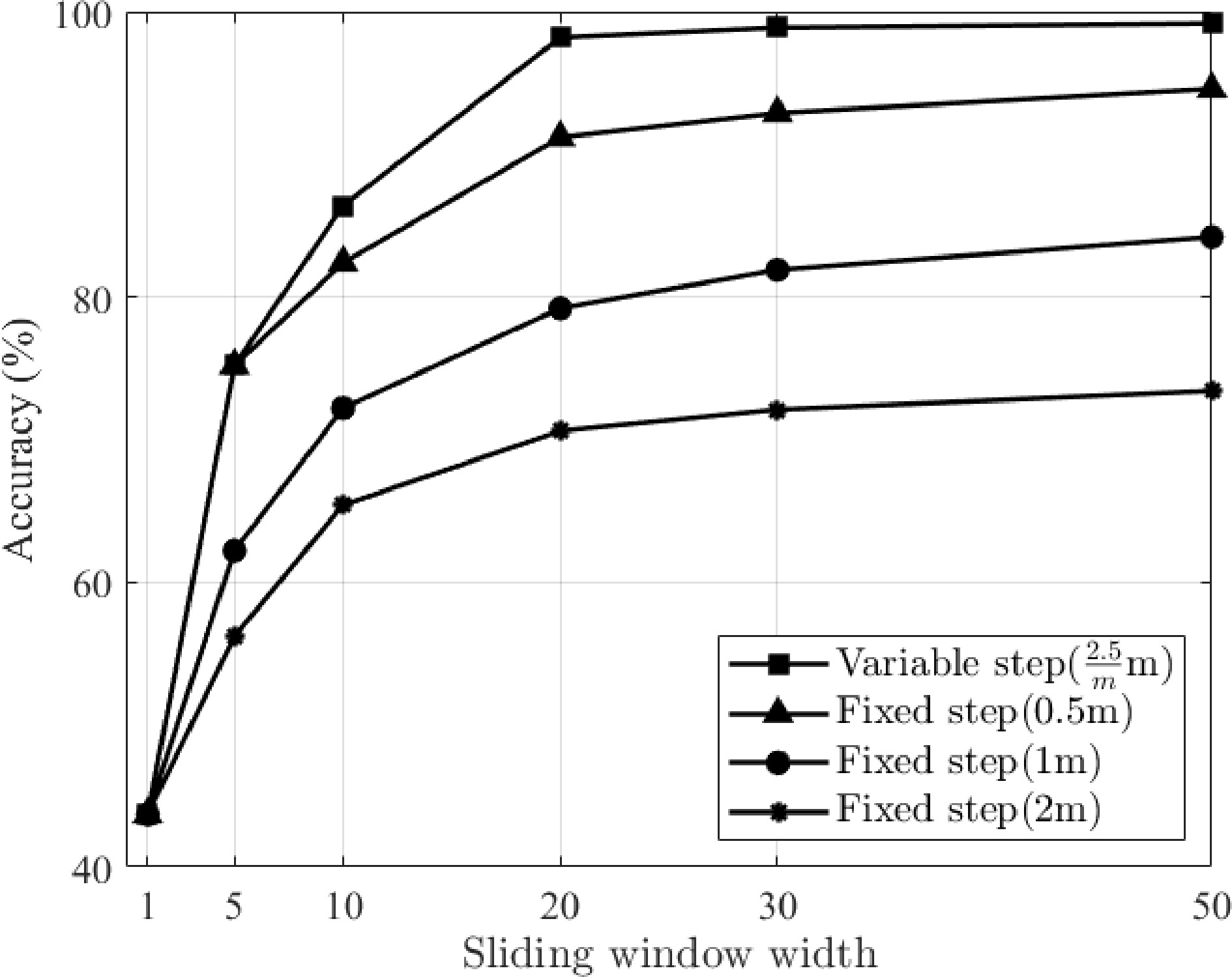
Figure 9. 

Recognition accuracy at different step sizes.

As the sliding windows' width m increases and the step size Δs decreases, it effectively captures localized and short-term terrain information around the intended landing site, demonstrating enhanced data reliability.

The results of the simulation indicate that terrain classification achieves optimal efficiency (accuracy > 96%) with a step size of 0.125 m and a sliding window width of 20. Increasing the width to 50 incurs approximately sixfold computational overhead while improving the accuracy by less than 2%. Consequently, the experimental configuration uses a step size of 0.1 m and a window width of 20 to balance real-time performance with classification accuracy.

Compared with the full-batch analysis that requires one to acquire and analyze the complete set of $ 4k $ data points (full batch), the DTFSF method exhibits the advantages summarized in Table 2. For resource-constrained UAVs navigating quasistatic yet evolving environments, this method strikes an optimal balance between adaptability and efficiency, a feat that cannot be achieved with traditional full-batch techniques.

Based on the dynamic response estimation and structural characteristics of the controlled plant, the sliding surface equation $ \mathbf{\Omega } $ and control law $ u $ are proposed:

where, $ \mathbf{\Lambda } $ is the coefficient of the linear sliding surface, and $ \mathbf{K } $ and $ \mathbf{\Phi } $ are the gain matrix of the control law. The terms $ {u}_{\text{eq}},\;{u}_{\text{sw}} $ denote the equivalent control input and switching control input, respectively.

According to Eq. (25), the motor control torque is obtained as follows:

where, $ \delta $ is the boundary layer's thickness. Let $ S\subseteq \left\{1,2,\ldots ,n\right\} $ denote the set of indices where $ \left| {\sigma }_{i}\right| \gt \delta $, and the saturation function is defined as follows:

The adaptive disturbance estimation $ {\hat{\tau }}_{D} $ complies with the following update law:

Here, $ \mathbf{\Gamma } $ is the gain matrix of the adaptive law, and $ {\hat{\tau }}_{D} $ is used to estimate the real constant disturbance $ {\tau }_{D} $, as the disturbance magnitude can be considered to be bounded and constant during the short landing period, i.e.

where, D is the disturbance bound.

Main results

Construct a quadratic Lyapunov function incorporating the sliding surface σ and the adaptive parameter estimation error $ {\tilde{\tau }}_{D}={\hat{\tau }}_{D}-{\tau }_{D} $ as follows:

The derivative of the Lyapunov function is obtained as follows:

From Eqs (14), (24), and (26), it follows that

The skew-symmetric property $ {x}^{\text{T}}({\dot{M}}_{L}-2{C}_{L})x=0,\;\forall x\in {\mathbb{R}}^{n} $, is a fundamental characteristic of Lagrangian mechanical systems. This property arises from the energy conservation structure of the Euler–Lagrange equations, where $ {C}_{L}(\dot{\mathbf{H }},\ddot{\mathbf{H }}) $ is defined such that $ {\dot{M}}_{L}-2{C}_{L} $ is skew-symmetric. Physically, it implies that the internal forces do not network on the system, thereby preserving the system's passivity. Mathematically, this property is derived by differentiating $ {M}_{L}(\dot{\mathbf{H }},\ddot{\mathbf{H }}) $ and constructing $ {C}_{L}(\dot{\mathbf{H }},\ddot{\mathbf{H }}) $ via the Christoffel symbols of the first kind^[34].

By substituting Eq. (32) into Eq. (31) and simplifying, we obtain

Theorem 1.

Consider the following Lyapunov function derivative:

where, $ x\in {\mathbb{R}}^{n} $, $ A\in {\mathbb{R}}^{n\times n} $, $ B\in {\mathbb{R}}^{n\times n} $, and $ \varepsilon \gt 0 $. The derivative $ \dot{V} $ is seminegative definite if the matrix $ A $ is a diagonal semipositive definite matrix and $ B $ is a semipositive definite matrix.

Proof

Let $ \xi =\text{sat}(x/\varepsilon ) $. The saturation function preserves the sign of $ {\xi }_{i} $, i.e., $ {\xi }_{i}{x}_{i}\geq 0 $ and $ 0\leq \left| {\xi }_{i}\right| \leq 1 $. Define two regions as follows:

Linear region: $ \left| {x}_{i}\right| \leq \varepsilon \Rightarrow {\xi }_{i}={x}_{i}/\varepsilon $;

Saturated region: $ \left| {x}_{i}\right| \gt \varepsilon \Rightarrow {\xi }_{i}=\mathrm{sgn}({x}_{i}) $.

Case 1: All components in the linear region

If $ {\left| x\right| }_{\mathrm{\infty }}\leq \varepsilon $, then $ \xi =x/\varepsilon $. Substituting into $ \dot{V} $, we have

For $ \dot{V}\leq 0 $, $ {x}^{\text{T}}(A/\varepsilon +B)x\geq 0 $ must hold for all $ x\neq 0 $. This requires $ A/\varepsilon +B $ to be semipositive definite. The satisfaction of the condition is a direct consequence of the known information.

Case 2: Partial or full saturation

Assume that some components of $ x $ are saturated. In this case

Since $ {x}_{i}\mathrm{sgn}({x}_{i})=\left| {x}_{i}\right| \geq 0 $, the diagonal term satisfies $ {x}_{i}{A}_{ii}{\xi }_{i}\geq 0 $ if $ {A}_{ii}\geq 0 $.

Combining both cases above, the proof is completed.

This indicates that the system's sliding mode kinetic energy decays to zero, causing tracking errors to vanish near-exponentially. Similar to adaptive PID-C, this ASMC strategy offers robustness against disturbances. Although its boundary layer reduces chattering, it slightly increases the tracking error. Timely controller switching or parameter adjustment can boost the response speed and minimize residuals.

The developed control law provides adaptive compensation against unknown disturbances, achieving full robustness against in-channel disturbances and partial robustness to unmodeled dynamics. Unlike existing SMCs, our design incorporates multiple dedicated tuning parameters for the tracking velocity $ \mathbf{\Lambda } $, transient dynamics $ \mathbf{K } $, steady-state error $ \delta $, system stability $ \mathbf{\Phi } $, and robustness $ \mathbf{\Gamma } $. Crucially, it operates without predefined trajectories, enabling seamless real-time path integration with fast convergence. As a model-specific robust controller, it can be combined with observers for enhanced stability. Future work may explore making its fixed parameters adaptive.

A drawback is potential control signal saturation from large initial errors, requiring clamping of the motor voltage. For the decoupled 2-DoF landing system, the controller is computationally lightweight, sustaining a 1,000-Hz frequency on embedded systems for high-precision real-time landings.

Numerical simulation

Although existing multirotor landing systems for 1−12 articles predominantly rely on hierarchical PID-C architectures, this work implements an ASMC scheme grounded in Lagrangian mechanics for the underactuated landing gear dynamics, with comparative simulations designed to rigorously quantify its nonlinear compensation capabilities against conventional linear control paradigms. This system is simulated with four scenarios:

(1) Case 1 (without disturbance): $ {\tau }_{D}=0 $;

(2) Case 2 (static disturbance): $ {\tau }_{D}=\begin{cases} 0 & t \lt 5\;\text{s}\\0.002 & t\geq 5\;\text{s}\end{cases} $;

(3) Case 3 (multiplicative fault): $ {\tau }_{M}=0.8u $;

(4) Case 4 (dynamic disturbance): $ {\tau }_{D} $ is Gaussian white noise with 0 mean and 0.001 variance.

In order to apply the proposed method, the parameters of the ASMC and PID-C are selected as follows:

THe initial height, initial velocity, and target height are

The initial disturbance estimation is

The PID-C parameters are tuned according to the ASMC framework. When the matrix $ \mathbf{\Lambda } $ is the identity matrix, $ {K}_{P}/{K}_{D} $ are set to 1. The system's stability is achieved by adjusting $ {K}_{P} $ to 0.5. To eliminate the steady-state error, $ {K}_{I} $ is set to 0.2, which achieves a good balance between response speed and stability.

Four scenarios with their corresponding results shown in Figs. 10−12 and Table 3.

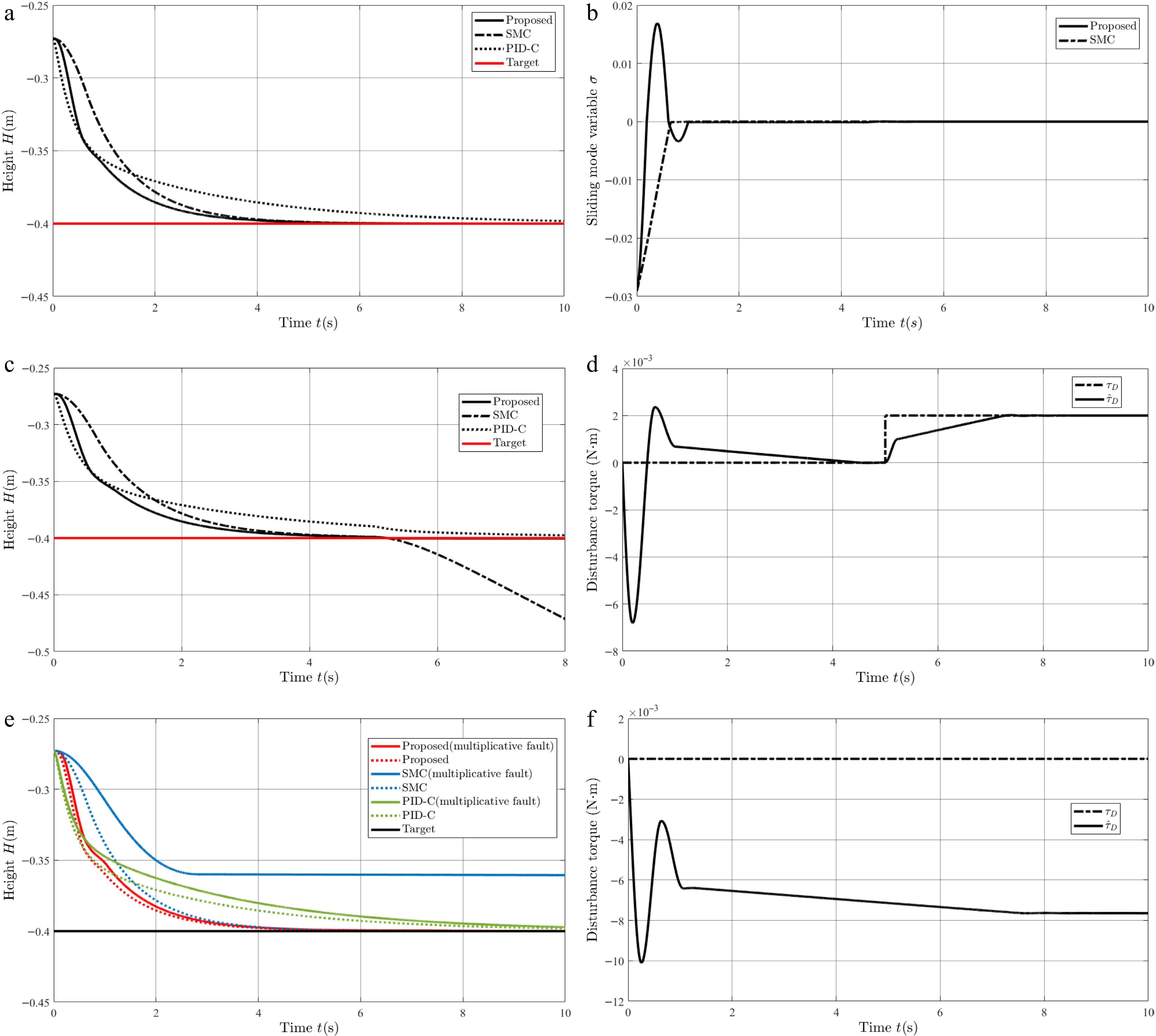
Figure 10. 

Simulation results: (a) H for Case 1; (b) $ \sigma $ for Case 1; (c) H for Case 2; (d) $ {\hat{\tau }}_{D} $ for Case 2; (e) H for Case 3; (f) $ {\hat{\tau }}_{D} $ for Case 3.

Under ideal disturbance-free conditions, the curves in Fig. 10a demonstrate exponential convergence behavior in trajectory tracking for all three controllers. The ASMC achieves the fastest convergence rate, whereas PID-C exhibits slower convergence to ensure stability. Figure 10b confirms that both ASMC and SMC ensure convergence to the sliding manifold under ideal conditions, driving the system's states along the manifold with mitigated chattering.

When subjected to instantaneous constant load disturbances (Fig. 10c), SMC fails to reject the disturbance because of its limited robustness and lack of adaptability, resulting in trajectory divergence. Other controllers maintain their performance. Figure 10d validates the adaptive estimation $ {\hat{\tau }}_{D} $ and convergence of the disturbance torque $ {\tau }_{D} $.

Under multiplicative actuator faults (Fig. 10e), SMC exhibits significant steady-state errors. Both ASMC (adaptive compensation) and PID-C (integral compensation) resolve this issue, with ASMC demonstrating superior fault tolerance.

The proposed method represents an evolved form of PID-C, combining its rapid response with enhanced precision. Conventional SMC proves to be unsuitable for physical implementations because of its limited robustness. ASMC excels in noncontact applications (e.g., positioning in mechanical systems). PID-C remains effective in contact-mode operations involving complex disturbances (e.g., shock absorption control of a helicopter's landing gear during touchdown).

As shown in Table 3, we used six metrics—root mean square error (RMSE), integrated absolute error (IAE), integrated squared error (ISE), integrated time-weighted absolute error (ITAE), integrated time-weighted squared error (ITSE), and control energy (CE)—to comprehensively evaluate the controller's steady-state error, convergence speed, energy consumption, and robustness. For each metric, the first value represents the group mean, and the second value represents the group's standard deviation.

The proposed method achieved significant improvements in the first five metrics. Across all 50 simulation tests, the controller maintained consistently lower errors, outperforming SMC by 18.3%, 25.4%, 33.7%, 30.0%, and 50.4%, and surpassing PID-C by 77.0%, 84.4%, 94.7%, 93.2%, and 97.3%, respectively, for RMSE, IAE, ISE, ITAE, ITSE, and CE. Statistical analysis confirmed the superiority of the proposed method across all valid metrics (all p < 0.001 after Holm–Bonferroni correction). The low standard deviations indicate strong robustness against disturbance uncertainties, whereas the significantly lower p-values verify statistically meaningful improvements over both SMC and PID-C in terms of steady-state error and convergence speed.

Notably, these performance gains were achieved with only a 2.2% increase in energy output according to the CE metric. This implies that ASMC improved all key metrics by over 18% with nearly unchanged energy consumption—an outcome of considerable value for the design of controllers in onboard energy-limited systems.

This simulation required MATLAB/Simulink (Version R2024a). The computational platform was a desktop computer equipped with an AMD Ryzen 5 5600X central processing unit. The ode45 (Dormand–Prince) solver was used, with a relative tolerance of 1 × 10⁻³ to ensure the solution's accuracy.

Conventional control frameworks often used fixed hierarchies and parameters, which can lead to performance degradation or failure in dynamic environments where the terrain's geometry, disturbances, or task objectives change unpredictably. To address this limitation, we propose an adaptive hierarchical control framework (AHCF) that enables cross-layer adaptation through real-time sensor fusion and context-aware policy switching. The AHCF integrates a three-tier strategic–tactical–operational (STO) management system, as illustrated in Fig. 11.

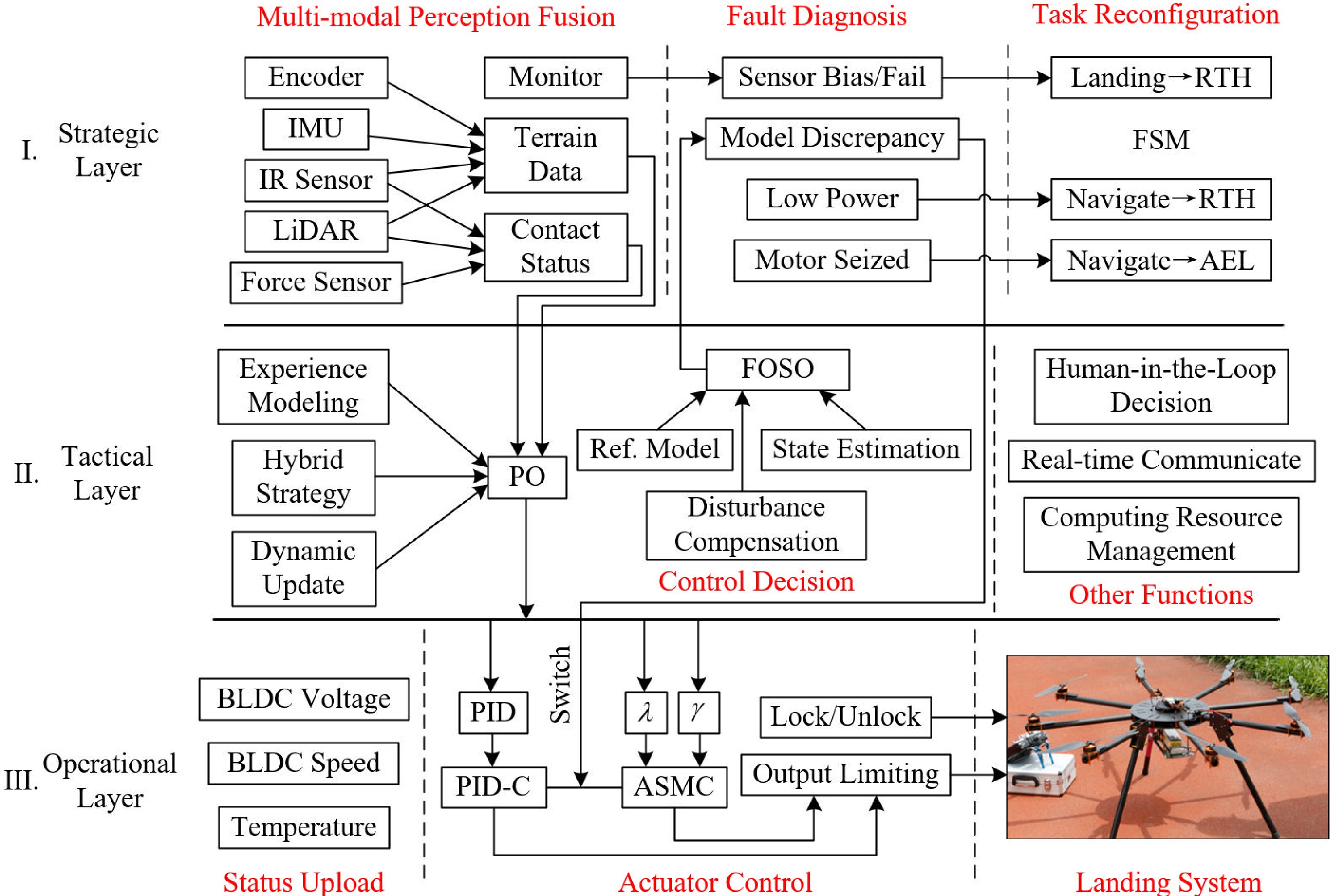
Figure 11. 

Diagram of the adaptive hierarchical control framework.

Strategic layer

This layer orchestrates multimodal perception fusion, fault diagnosis, and mission reconfiguration. It synthesizes the terrain data and contact states from redundant sensor networks to maintain robust environmental awareness. A unified monitoring interface streams real-time state data to support fault diagnosis for both the flight control system (FCS), such as IMU drift and the landing system, including sensor failures, model discrepancies, and the actuator jamming. Critical system warnings include communication link loss (> 5 s), low battery, and abnormal motor voltage warnings.

As shown in Fig. 12, the mission reconfiguration subsystem governs the UAV's finite state machine (FSM), managing transitions between key states: initiation (INIT), normal, pre-landing (PRELAND), landed, autonomous emergency landing (AEL), return to home (RTH), and faulty (ERR). Critical faults trigger a transition from NORMAL to ERR, halting the UAV until resolution, whereas unresolved warnings initiate a NORMAL→RTH transition.

Operating at 10 Hz, this layer integrates peripheral data processing, calculating the terrain's flatness (DTFSF), and low-level hardware ISRs, updating a high-priority 1-byte status register.

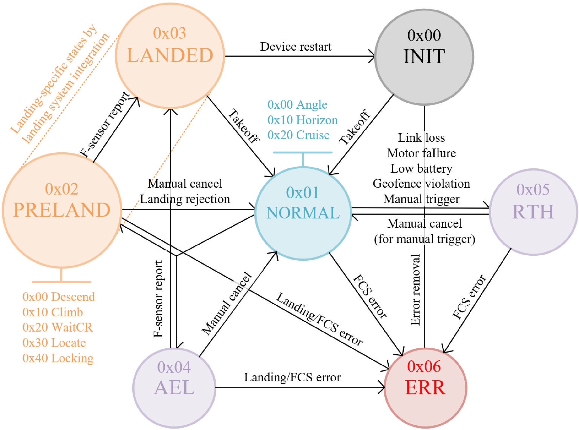
Figure 12. 

Basic finite state machine framework for an intelligent multirotor UAV.

Tactical layer

This layer implements a dual-module control architecture. A parameter optimizer (PO) used data-driven strategies to dynamically adjust the control parameters during contingencies. The PO module monitors the terrain's features and the system's response in real time, dynamically adjusting the ASMC's parameters and the DTFSF thresholds. For instance, upon detecting complex terrain, the PO can appropriately relax $ {\kappa }_{1} $ to allow landing with a larger tilt angle while increasing the robustness gain of the ASMC to handle greater disturbances. A full-order state observer (FOSO), based on an approximate linearization of the landing leg's dynamics, provides real-time state estimates via a Kalman filter (KF) to evaluate the ASMC's performance. If the deviation between the ASMC output and the FOSO estimate exceeds a predefined robustness margin—indicating excessive model perturbation—the system immediately switches to the more conservative PID-C controller to prioritize stability. The switching logic is based on a threshold judgment of the FOSO estimation error, and a hysteresis comparator is adopted to avoid frequent switching. At the moment of switching, the system retains the output from the previous control cycle as the initial value, ensuring state continuity and a smooth transition while preventing any instantaneous jitter caused by the switching process.

Operational layer

Directly interfacing with the hardware, this layer monitors the brushless direct current (BLDC) motor's parameters (e.g., winding temperature, rotor position) and ambient conditions via auxiliary sensors. The control logic combines tunable PID controllers with ASMC, reinforced by output constraint enforcement. Mechanical safety is ensured through centralized locking and unlocking of the landing gear mechanism.

The STO architecture implements software-level scheduling via priority-based and timer-driven interrupts. To guarantee the control system's stability, the ASMC is assigned the highest priority, maintaining a stable 1-kHz execution frequency. Lower-priority processes (e.g., multimodal perception) are segmented and executed during the controller's idle cycles. Crucially, UAV fault detection is granted the highest interruption priority, enabling it to preempt all landing control system (LCS) operations in the event of an FCS failure. The AHCF's time synchronization structure is depicted in Fig. 13. Let the time proportions of the STO programs be denoted as P_S, P_T, P_O, respectively. We then have

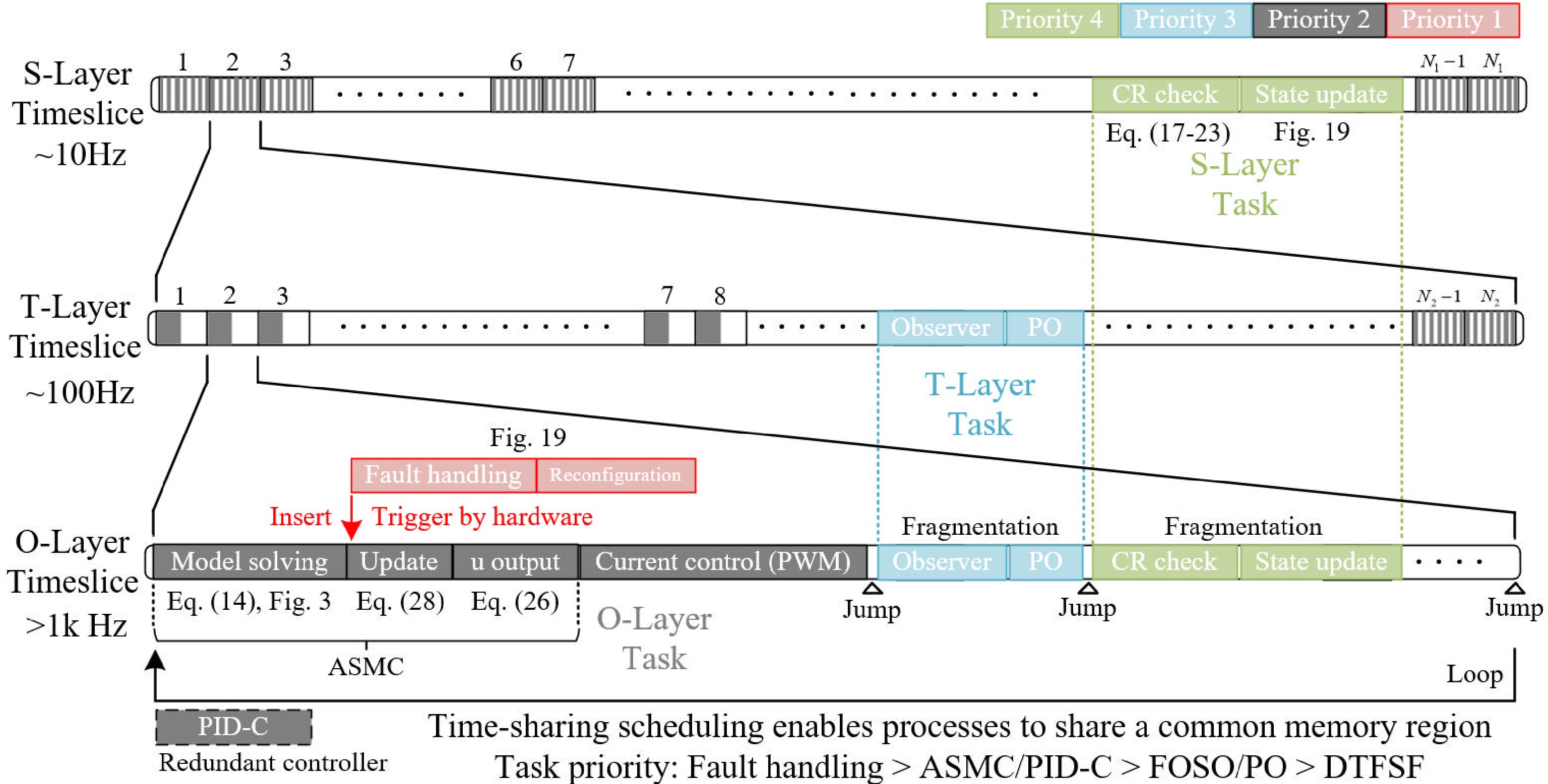
Figure 13. 

Diagram of the AHCF's time synchronization with task priority.

Prelanding phase

This section details the sensor requirements and programming logic for the PRELAND phase. IMU, barometer, and global positioning system (GPS) data are fused by the flight controller for 6-DoF state estimation (three-dimensional position + three-dimensional orientation), determining the timing of the landing system's activation. Current landing methods include vision-only, beacon-based optical, and hybrid approaches (the sensors' trade-offs are shown in Table 4). Pure optical landing (LiDAR + IR) offers the highest energy efficiency.

As per the control strategy, landing Legs 1 and 2 use a controllable rocker mechanism for optimal impact absorption, whereas Leg 3 has a fixed buffer (the working logic is shown in Fig. 14).

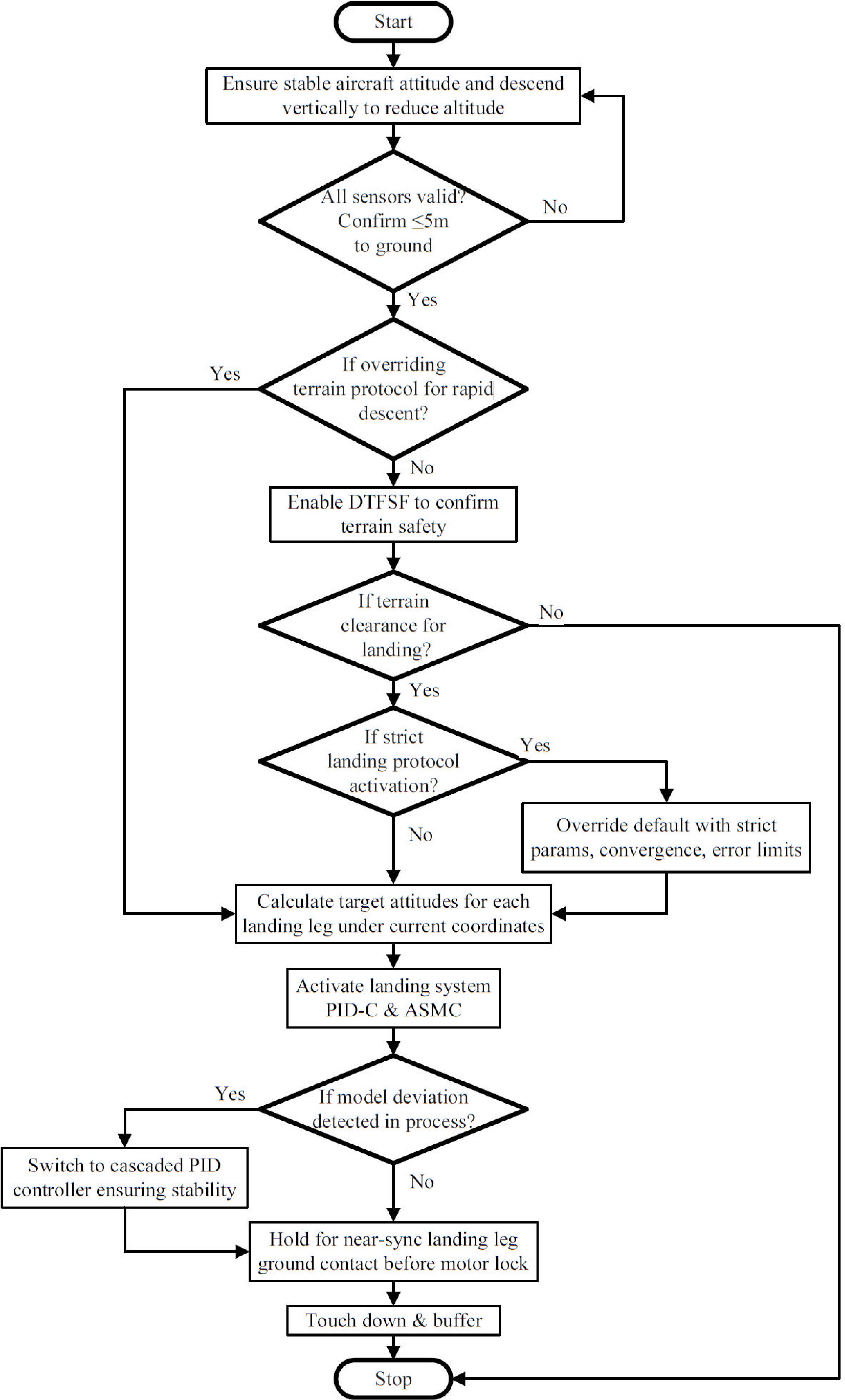
Figure 14. 

Working principles and flowchart of the landing process.

In operation, the landing subprogram first uses LiDAR's IR ranging to measure footpad-to-ground distances. When all distances are below 5 m, the DTFSF activates to classify the terrain (enabling image-free autonomy) into three types on the basis of Control Register (CR) thresholds: Basic terrain (default strategy), obstacle terrain (strict strategy, adjusted precision/error limits), and extreme terrain (landing rejected).

The controller then sync-adjusts the legs until the vertical distance difference between the sensors is under 5 mm. Finally, the actuators lock for simultaneous touchdown, engaging all strut buffers upon contact.

During the adjustment of the rocker-actuated mechanism, severe deviations in the computed system model that exceed the robustness range of the ASMC may lead to significant chattering and instability. To mitigate this, an actuator saturation link and a controller switching strategy are implemented to maximize the controller's stability. If the UAV requires rapid landing, the landing subprogram can be switched to fast mode before activation at the terminal. This mode enables a rapid descent from an altitude of approximately 5 m within 5−10 s, but it is only suitable for safe terrains (flat surfaces or gentle slopes). To ensure terrain awareness, this mode requires the integration of low-latency remote video transmission capabilities in both the terminal and the UAV.

This section outlines the UAV platform's specifications, the computational load characteristics of the safe landing algorithm, and the results of the flight test. The platform's architecture and integrated sensors are first described, followed by a description of the system's performance parameters and configuration schemes for evaluating and identifying the landing zone typologies. Subsequently, the real-time processing capabilities of multiple modules within the AHCF are demonstrated through comprehensive test scenarios. Finally, the landing test data acquired in nominal environments are presented.

Configurations and real-time computation

The flight controller uses a Radiolink F722 octocopter system with an STM32F722RE MCU (216 MHz), an ICM42688 IMU, and an SPL06-001 barometer (altitude accuracy = 5 cm). Attitude angles from sensor fusion achieve ~0.1° accuracy. Critical flight data are output via Universal Asynchronous Receiver/Transmitter (UART)/USB for the multisubsystem LCS design.

We present a low-power, real-time embedded platform for UAV vertical takeoff and landing (VTOL) systems. The core is an STM32H743VI MCU (480 MHz Arm® Cortex®-M7 with an Floating Point Unit [FPU], 2424 CoreMark), balancing high computation and energy efficiency. It meets the demands of complex algorithms like ASMC and DTFSF. Key low-power features include:

(1) 275 µA/MHz in Run mode (sustained power < 1 W);

(2) 2.43 µA in standby mode.

Its 1 MB of Static Random-Access Memory (SRAM) and over 35 peripherals (e.g., high-speed Serial Peripheral Interface [SPI], Inter-Integrated Circuit [IIC], 16-bit Analog-to-Digital Converters [ADCs]) enable seamless sensor integration, forming a complete perception–control loop.

During standard high-altitude flight, the landing system is locked, and the controller is downclocked to 48 MHz to save energy. LiDAR runs at a reduced 5 Hz for avoidance, and the nonessential landing sensors are off. A 3-m altitude threshold triggers this power-saving mode, with the variable-frequency control logic detailed in Table 5.

A detailed analysis of the algorithm's execution time using the STM32H743VI (480 MHz Cortex-M7, FPU enabled) is presented in Table 6.

The real-time performance analysis reveals that the ASMC controller dominates the computational load (14% CPU usage at 1 kHz), constrained by double-precision FPU operations. In contrast, the PID controller achieves exceptional efficiency (1.2% usage) through lean implementation. Acceleration of the hardware proves critical: FOSO leverages Common Microcontroller Software Interface Standard - Digital Signal Processor (CMSIS-DSP) with FPU/DSP to maintain 3.2% occupancy at 100 Hz, whereas DTFSF exploits the Art Accelerator (ART)/I-cache to manage cycles of 2.4 ± 0.2 ms efficiently despite its memory-intensive workload. Crucially, the aggregate 20.8% total occupancy leaves substantial headroom (79.2%) for auxiliary tasks, validating the architecture's real-time capability. The ASMC's execution variance (± 15 μs) emerges as the primary optimization target for deterministic control.

Test results

As illustrated in Fig. 15, the prototype UAV in this study was flown along a predefined route A→B→C→D→E, with a total ground-projected trajectory length of 127.8 m. To evaluate the terrain recognition capability, Segments BC and CD traversed an undulating grass field, followed by landing at the relatively flat Location E. The primary landing safety metric CR_0.95 was used, with values exceeding 80% indicating secure terrain. The experimental results encompass the full-process data from the system's initiation to landing, including:

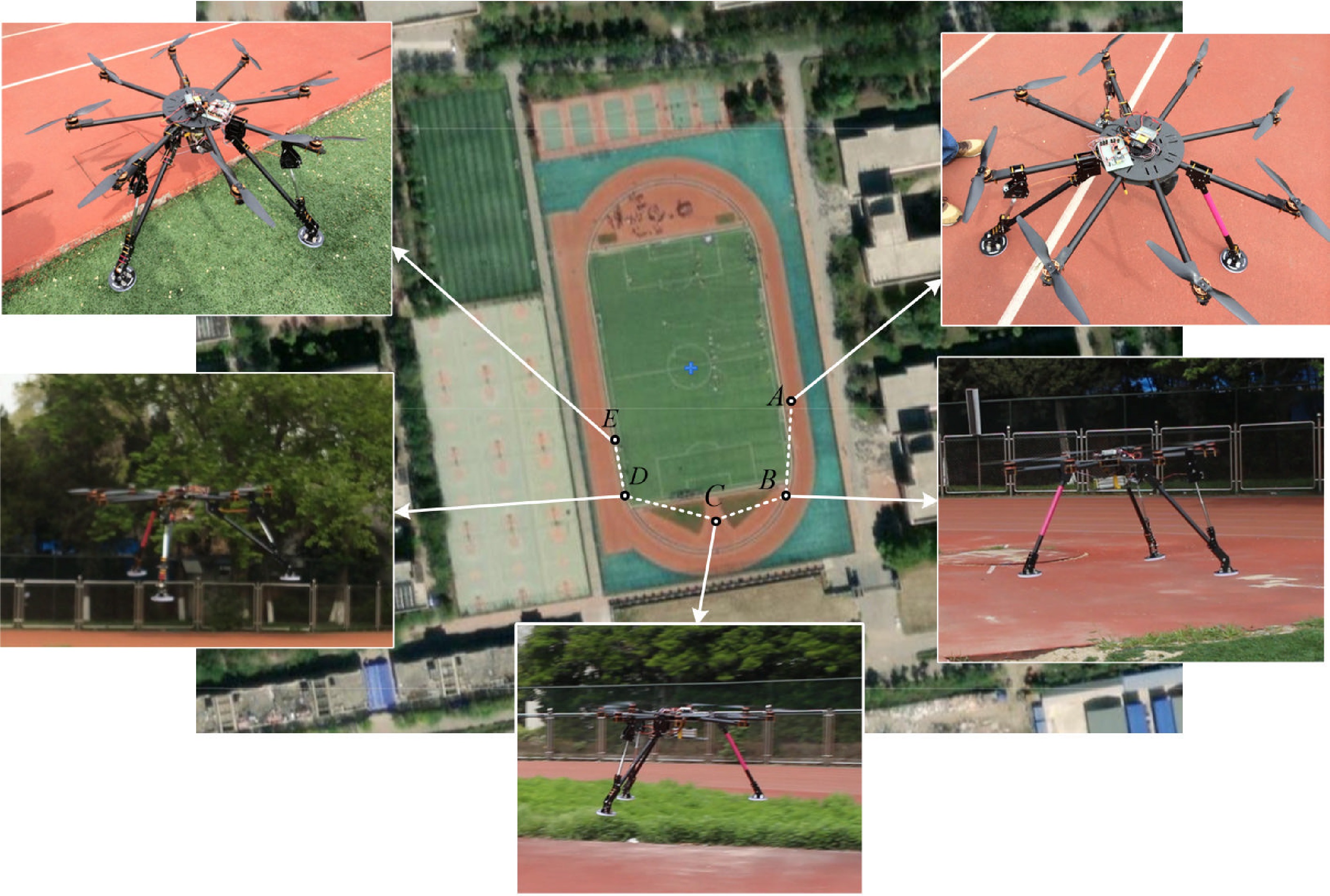
Figure 15. 

Landing procedure in a real environment.

(1) the UAV's relative altitude (sourced from the flight controller's serial output);

(2) the CR_0.95 curve (initialized 10 s after takeoff at 10 Hz, generated by the LCS);

(3) The landing system's total power consumption (covering the LCS, sensors, and two BLDC motors in the landing legs);

(4) The system's status (1 byte of data, output by the LCS).

Figure 16a−c presents both the raw data and filtered data processed with a moving average filter (window size = 10).

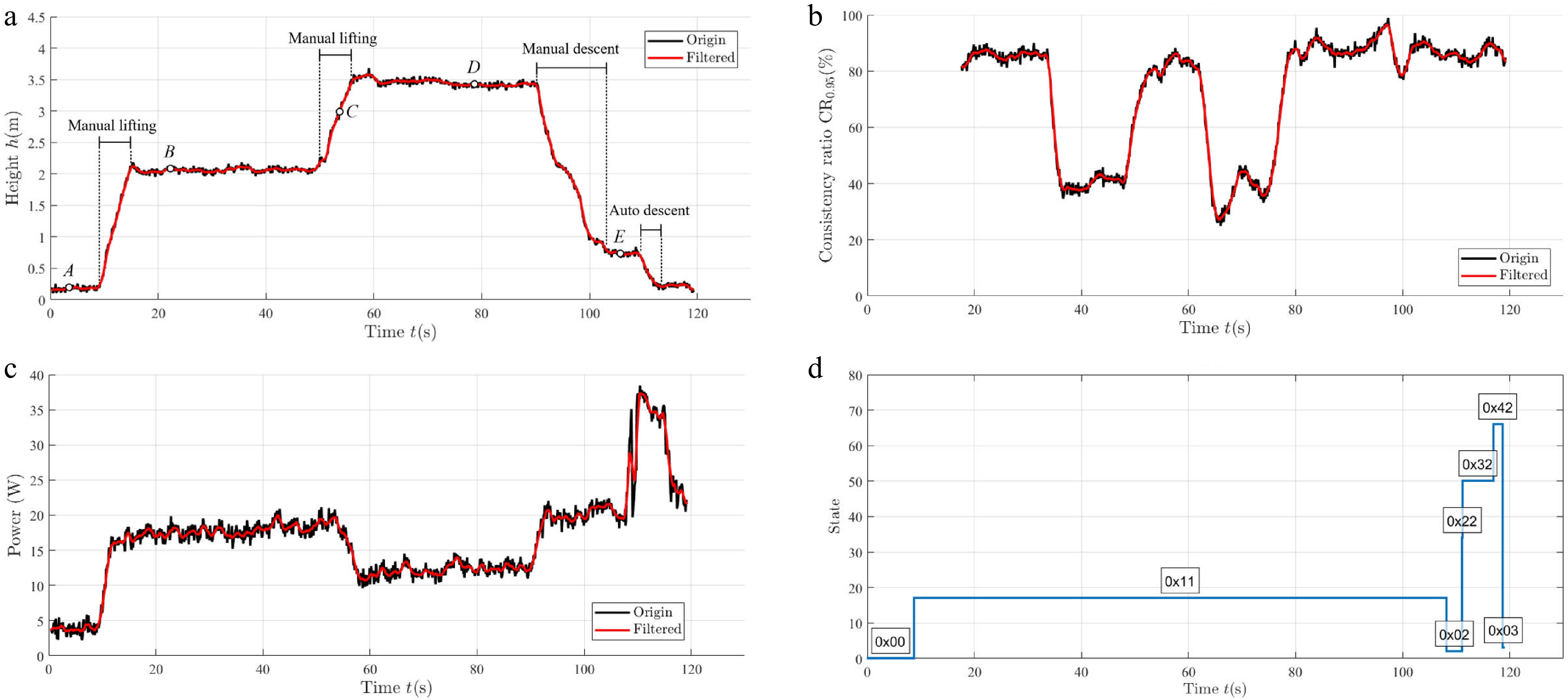
Figure 16. 

Data from the entire process from INIT to LANDED. (a) Flight; (b) perception; (c) power; (d) status.

As depicted in Fig. 16a, Points A–E on the map correspond to the labeled positions in the trajectory plot. During the mission, the UAV executed two manual ascents, one manual descent and one autonomous descent. The first ascent (0.2−2 m) validated the system's stress response under the 3-m threshold (see Row 1, Table 5). The second ascent (2−3.5 m) assessed low-power operation above the threshold. The manual descent to 0.7 m minimized the sensors' measurement errors near the ground. Subsequent autonomous descent triggered landing procedures with rapid leg actuation for a low-impact touchdown.

In Fig. 16b, the CR index computed at 10 Hz by the DTFSF reflects undulation within a 2-m radius—approximately triple the UAV's size—satisfying the measurement area requirement in Section 2.1. The horizontal velocity averaged 1 m/s. Notable drops in CR (80%–50%) occurred over segments BC/CD, whereas the values exceeded 80% on flat terrain, confirming the metric's sensitivity to localized terrain complexity.

Figure 16c demonstrates the power consumption, aligning with Table 5's low-energy profile.

(1) Ground standby < 5 W. With LiDAR deactivated before takeoff, the controller and peripherals maintained their power consumption below 5 W.

(2) Low-altitude flight: 15−20 W. At altitudes of < 3 m, all sensors were activated.

(3) High-altitude flight: 10−15 W. Above 3 m, the leg-mounted ranging/force sensors were disabled, whereas LiDAR operated at a scaled-down frequency, reducing the power draw by 5 W.

(4) Landing phase: 20−40 W. The dual 12-V landing leg BLDC motor exhibited a peak power draw of 20 W.

As indicated in Fig. 16c, the LCS's average power consumption of 15 W enables the miniaturization of UAVs below 0.2 m, subject to a dual-series (> 5 V) power supply and a > 300 g payload capacity (encompassing the compact landing leg, low-power LiDAR, sensors, and airframe).

Figure 16d documents state transitions: INIT → normal (horizon mode) → PRELAND (descent, leg positioning, locking) → LANDED. Horizon mode maintained a stable attitude during rapid manual maneuvers (ascent, descent, lateral motion), proving essential for A→ E navigation.

These experimental results demonstrate that the octocopter with adaptive multilevel control achieved the following:

(1) Low-power terrain scanning;

(2) 10-Hz mode switching;

(3) Precision leg control;

(4) Real-time embedded operation (a 1-kHz control loop, 20% CPU load).

This validates the simulations in the previous sections.

We propose an AHCF with integrated sensor fusion for intelligent multirotor UAV landing systems.

(1) A bio-inspired rocker bogie landing mechanism reduces the complexity of control while ensuring kinematic redundancy for robust terrain adaptation. The Lagrangian-based dynamic model, enhanced by real-time attitude perception, enables precise compensation for gravity and low-coupling motion control.

(2) The DTFSF algorithm fuses IMU, LiDAR, range finder, and force sensor data to ensure computational efficiency and resilience to noise. Validated on diverse terrains, the algorithm distinguishes basic (flat/ramp), obstacle (continuous/discrete), and extreme terrain types with > 95% accuracy at a window width of 20.

(3) The ASMC controller with saturation-function-based disturbance adaptation guarantees Lyapunov stability. Numerical simulations demonstrated ASMC's superiority over conventional and nonadaptive methods in terms of rapid convergence (< 4 s), suppressed chattering, and robustness to disturbances and actuator faults (20% loss).

(4) The STO framework integrates multimodal sensor fusion, fault diagnosis, and ASMC, achieving synchronized data interaction across the strategic, tactical, and executive layers at < 1-ms latency.

Unifying mechanical design, environmental perception, and adaptive control with high-efficiency implementations, the system achieves real-time operation at 1 kHz on a Cortex-M7 MCU. This provides a unified solution for safe landing in unstructured environments, enabling miniaturization and concealment of landers.