-
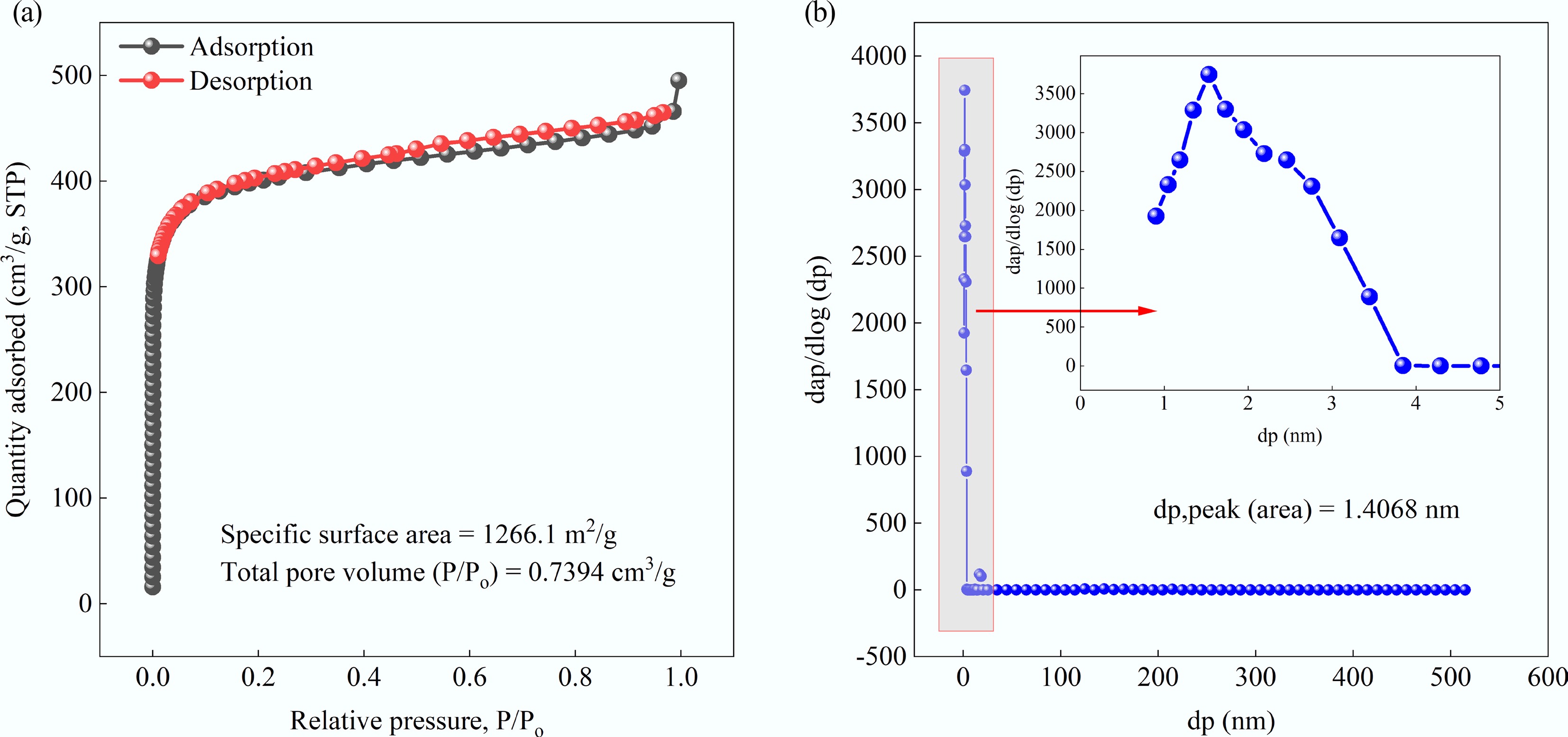
Figure 1.
(a) Adsorption and desorption curves, and (b) pore size distribution of MAHC.
-
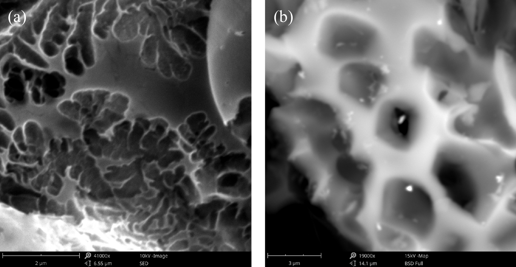
Figure 2.
SEM images of MAHC at different magnifications. (a) 41,000×, and (b) 19,000×.
-
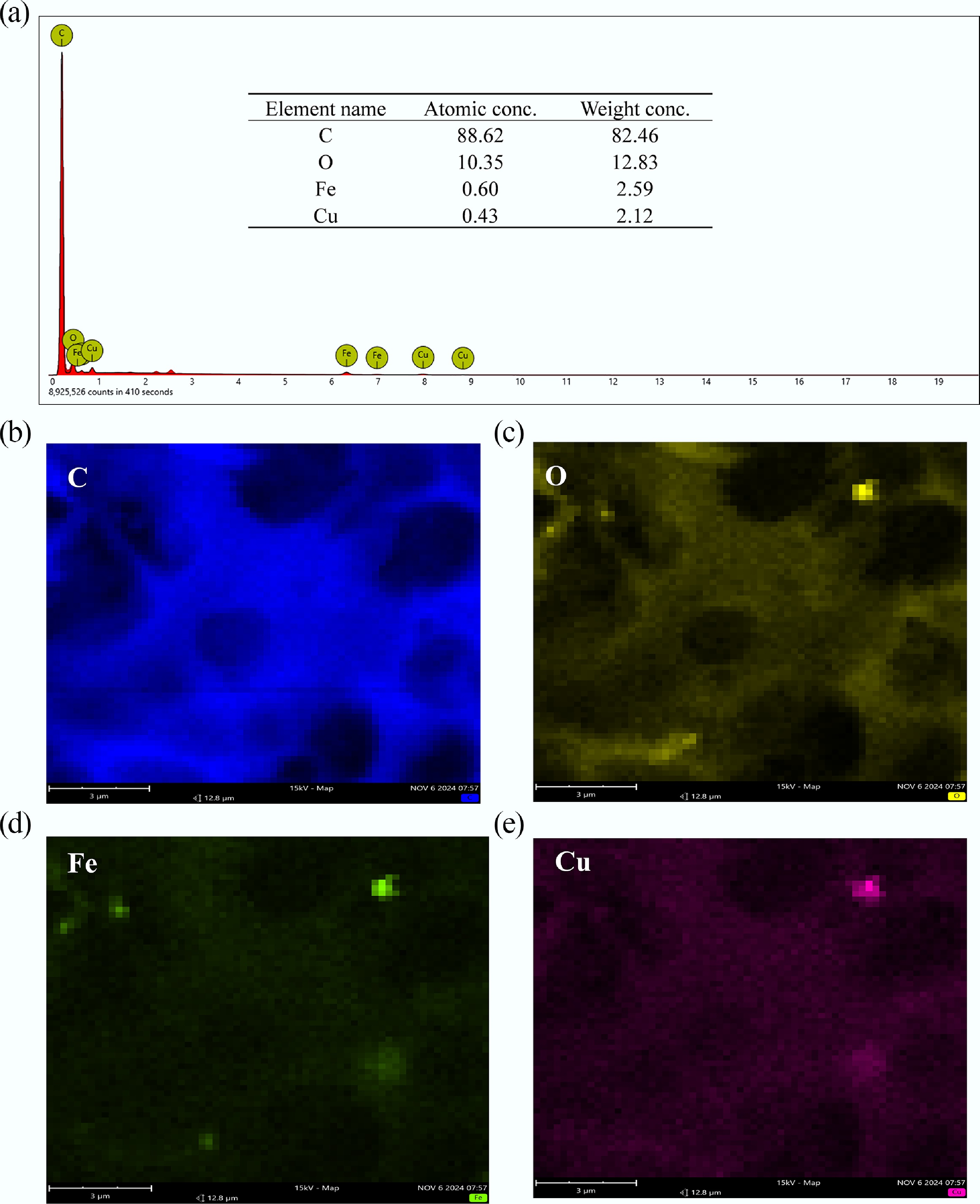
Figure 3.
(a) EDX results of MAHC element composition at the surface, (b) C, (c) O, (d) Fe, and (e) Cu.
-
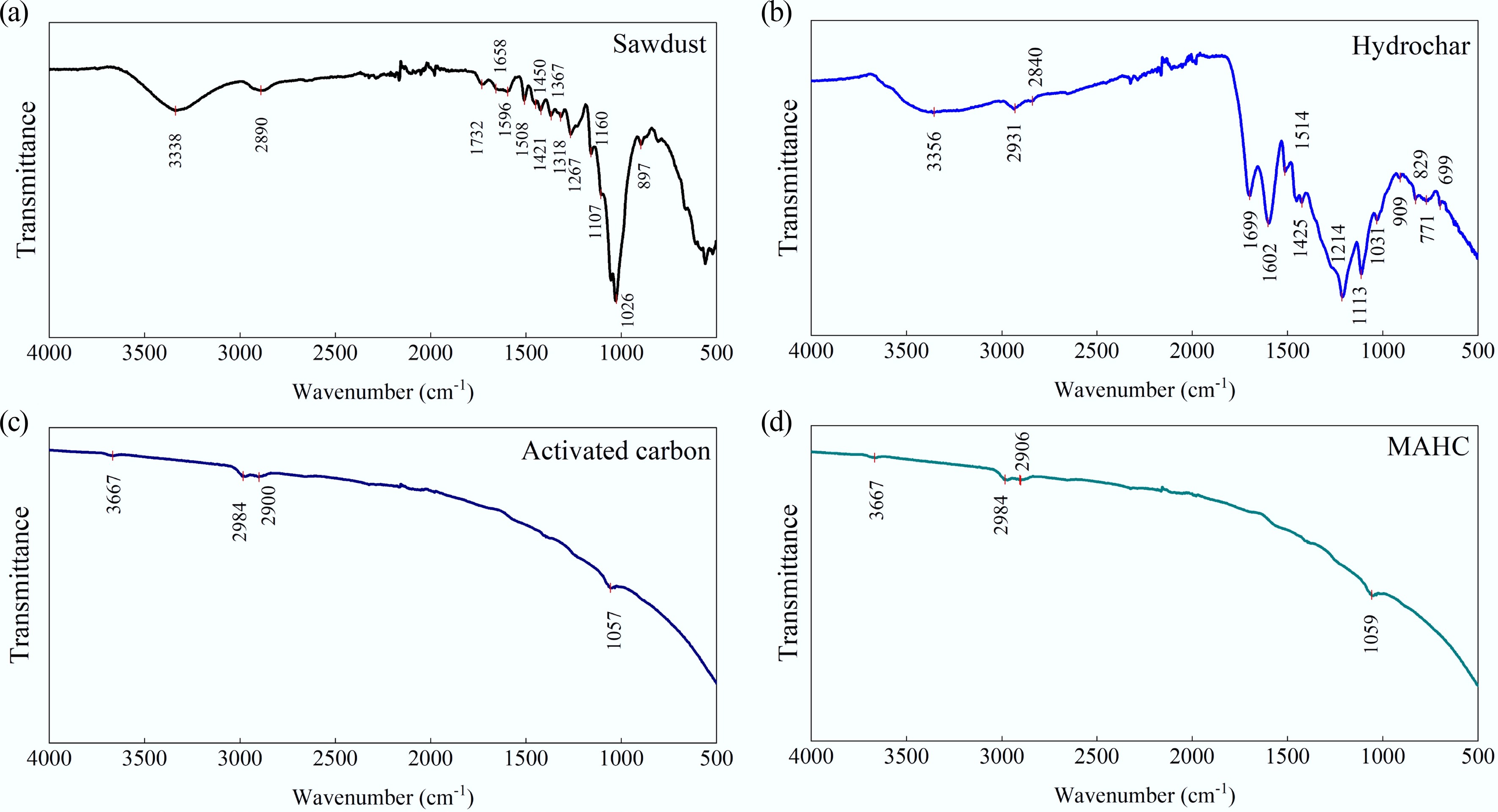
Figure 4.
FTIR spectra of (a) sawdust, (b) hydrochar, (c) activated carbon, and (d) and MAHC.
-
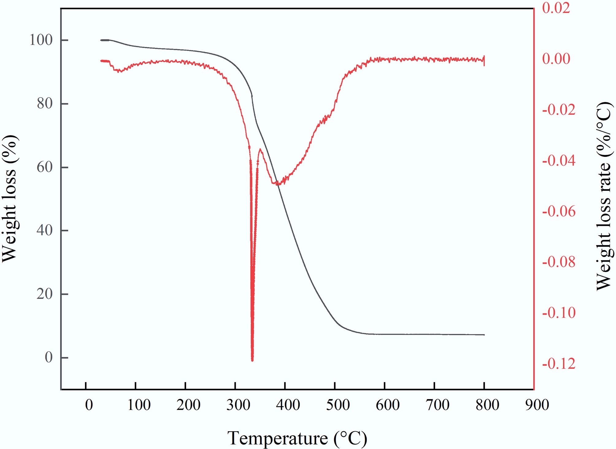
Figure 5.
Thermal degradation characteristics of MAHC.
-
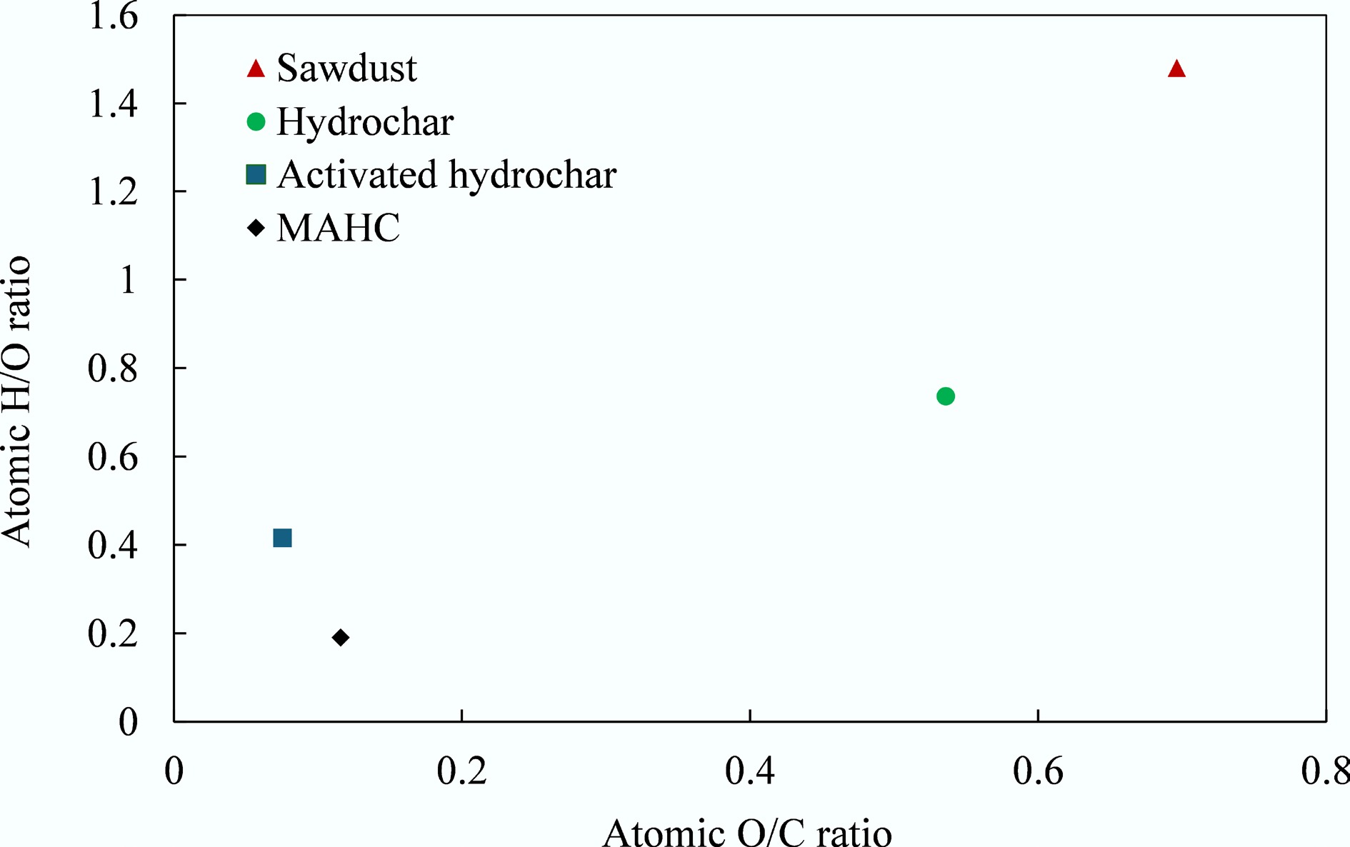
Figure 6.
Van Krevelen diagram.
-
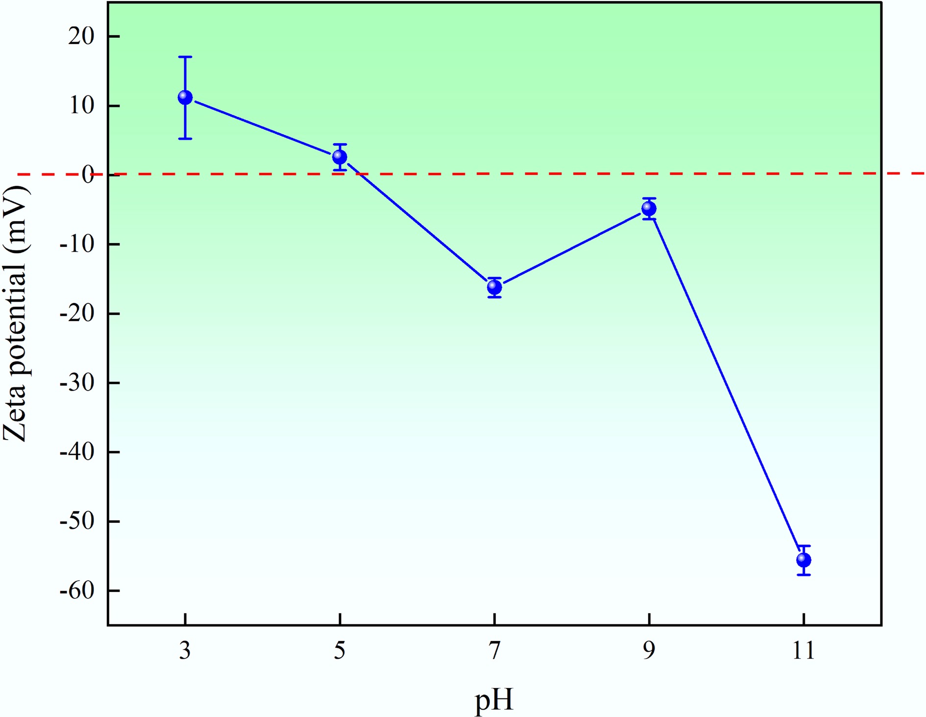
Figure 7.
Zeta potential results of MAHC at different pH levels.
-
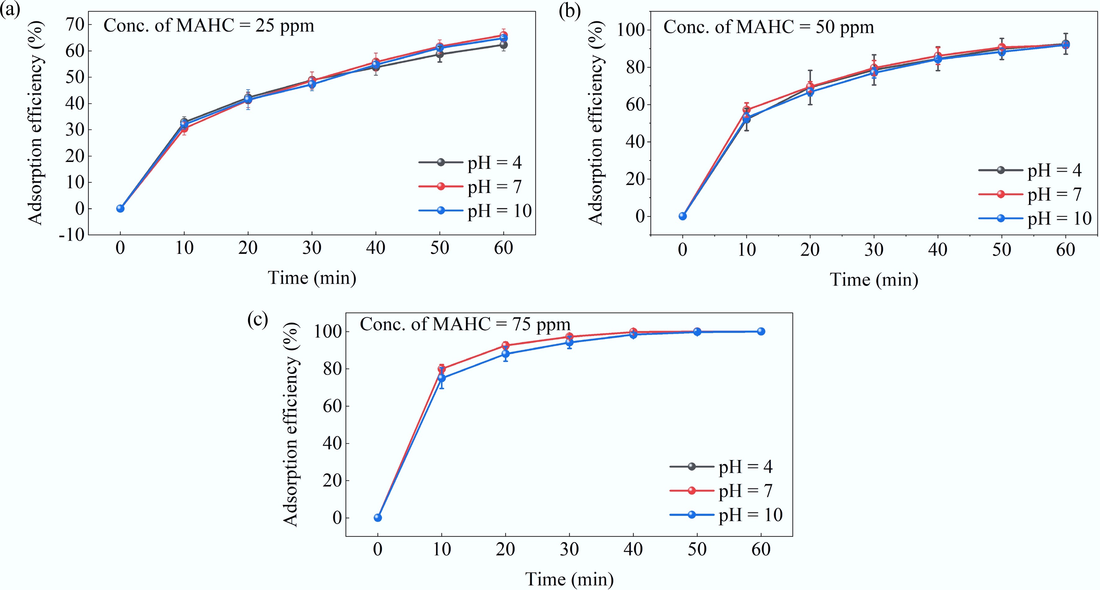
Figure 8.
Effect of pH level on the adsorption efficiency of MAHC obtained at MB concentration of 5 ppm, 24 °C, and (a) 25 ppm MAHC, (b) 50 ppm MAHC, and (c) 75 ppm MAHC.
-
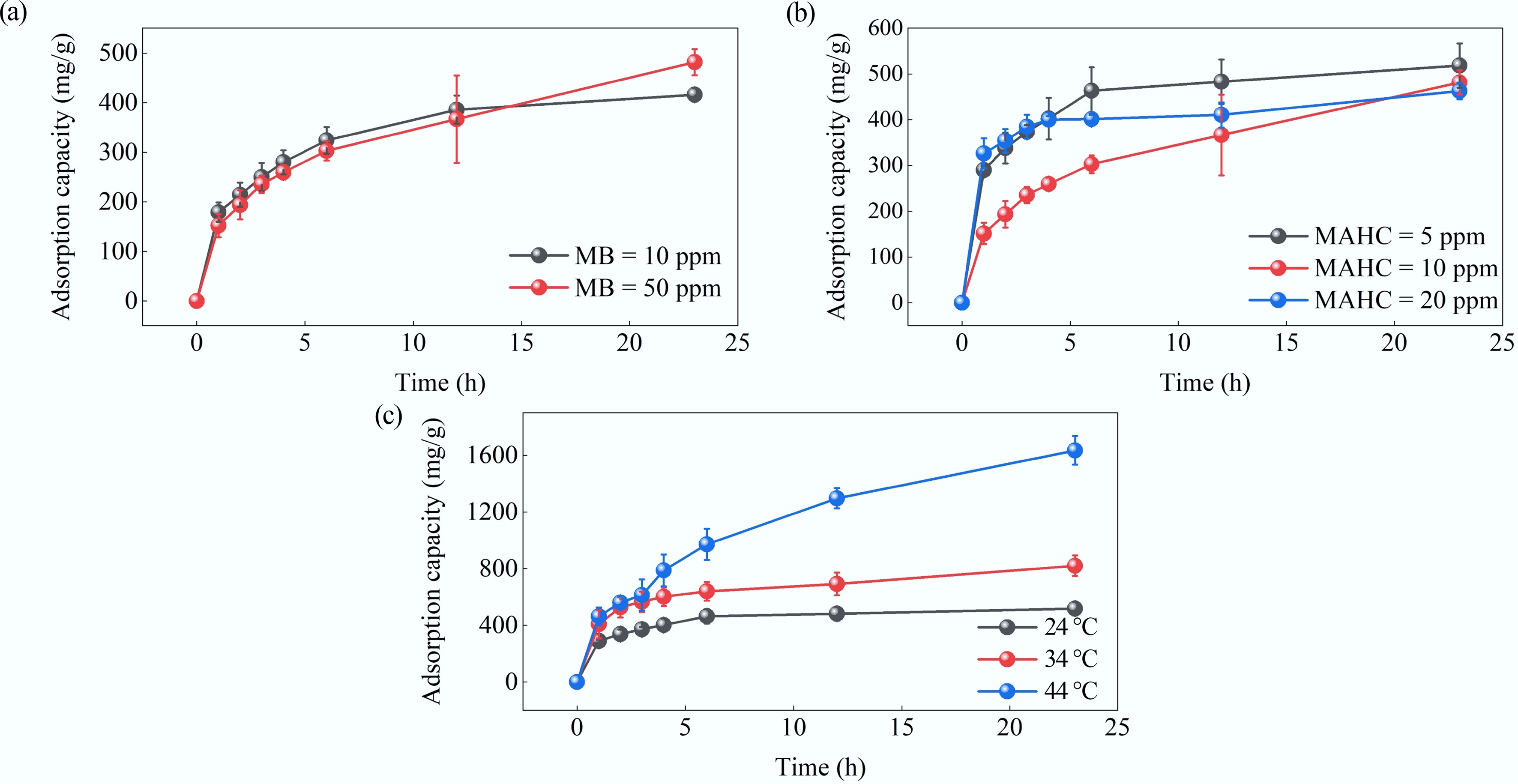
Figure 9.
Effect of (a) MB concentration, (b) MAHC amount, and (c) temperature on adsorption capacity.
-
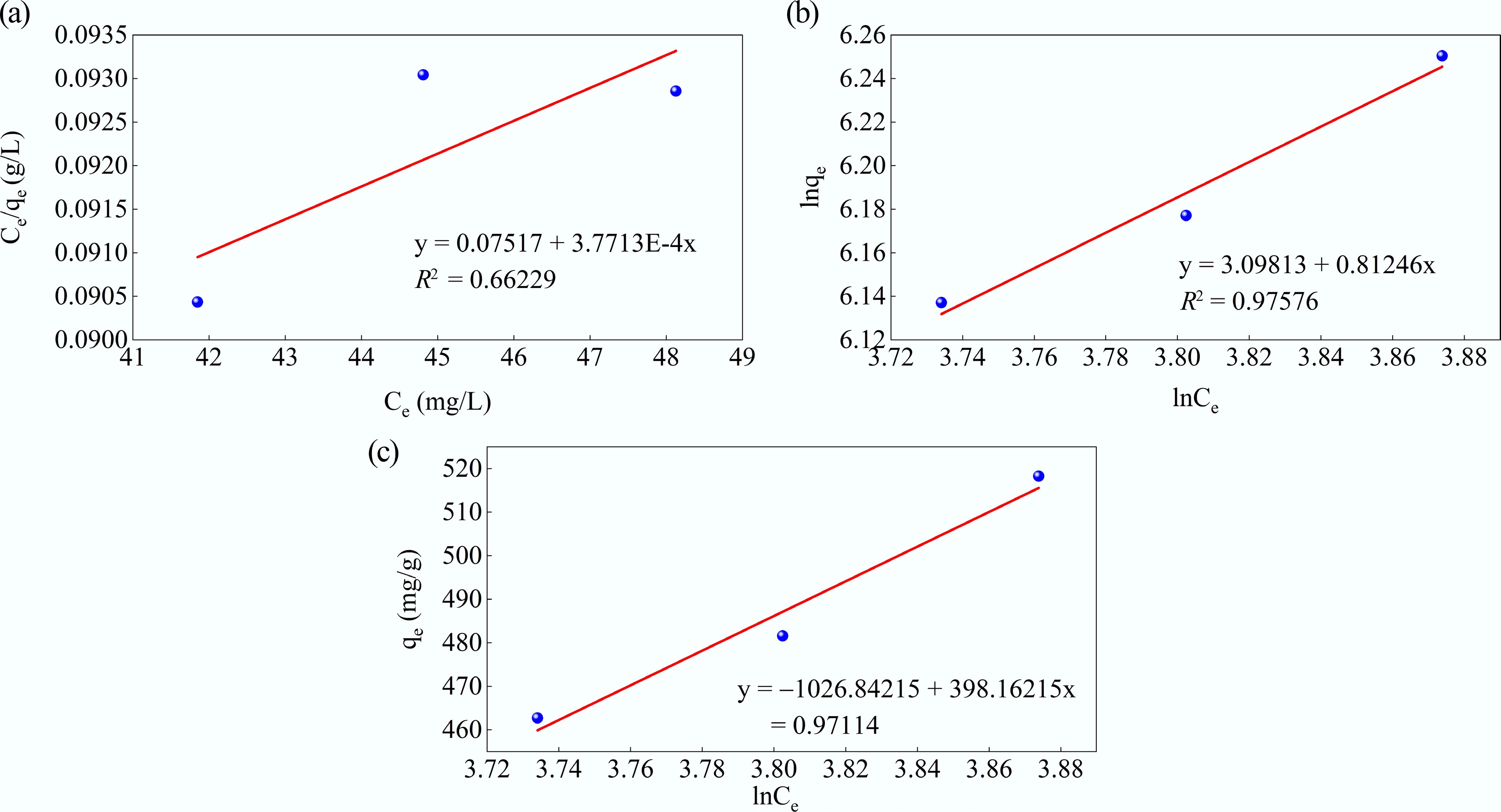
Figure 10.
(a) Langmuir, (b) Freundlich, and (c) Temkin adsorption isotherms for MB adsorption at 50 ppm MB, pH = 10, MAHC = 5–20 ppm, and 24 °C.
-
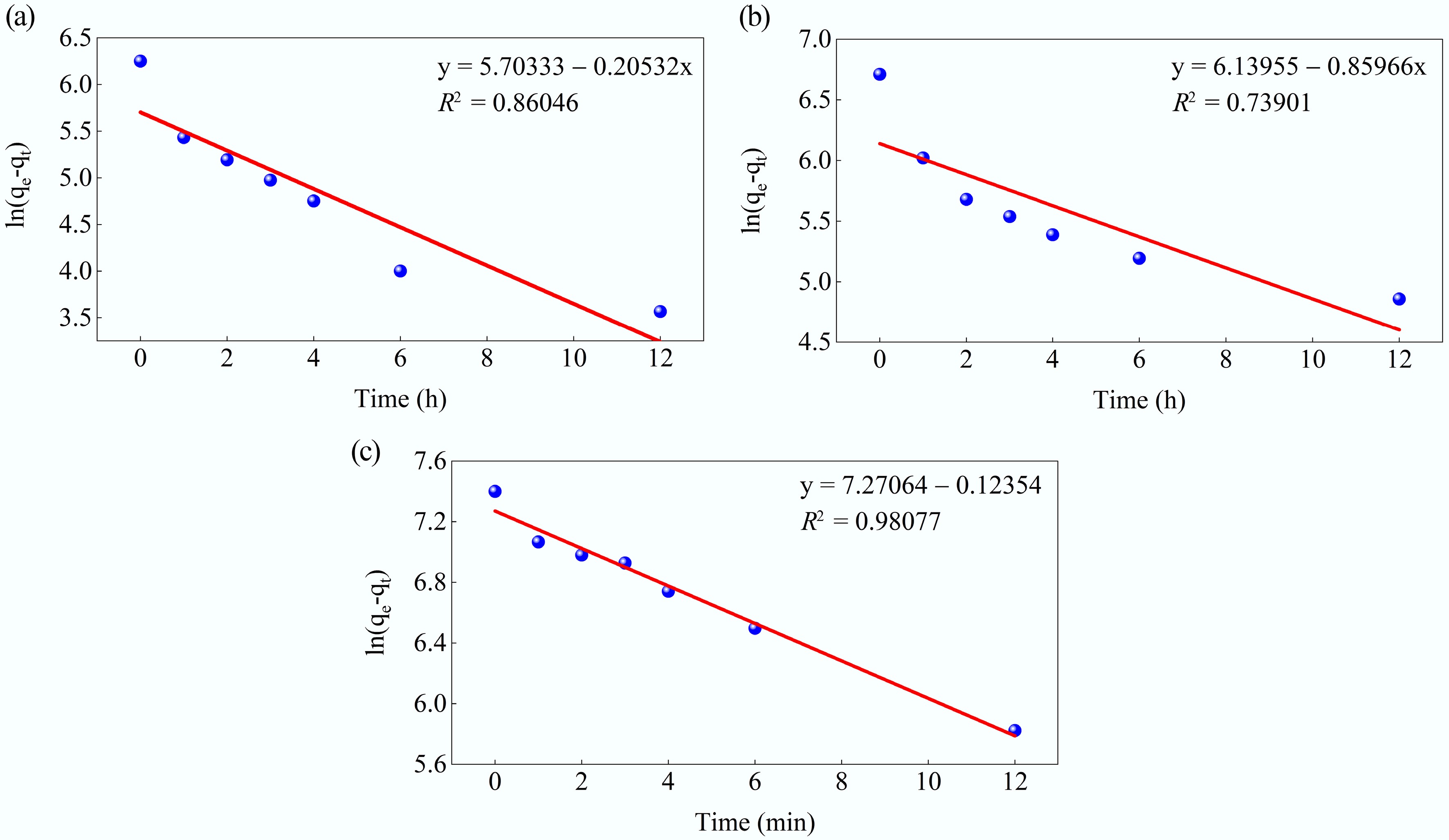
Figure 11.
Kinetic fits for MB adsorption on MAHC at (a) 24 °C, (b) 34 °C, and (c) 44 °C, using the pseudo-first-order model.
-
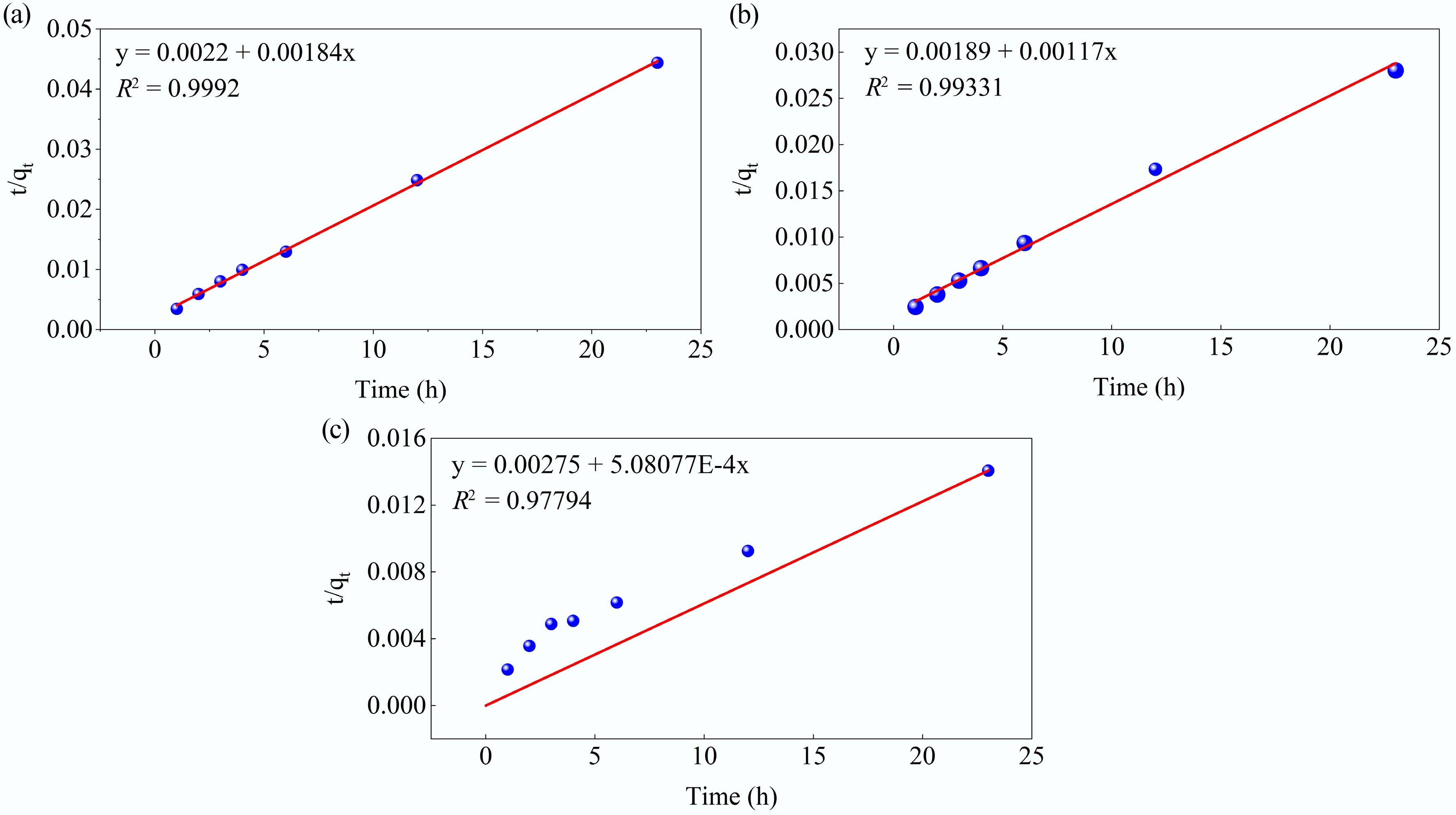
Figure 12.
Kinetic fits for MB adsorption on MAHC at (a) 24 °C, (b) 34 °C, and (c) 44 °C, using the pseudo-second-order model.
-
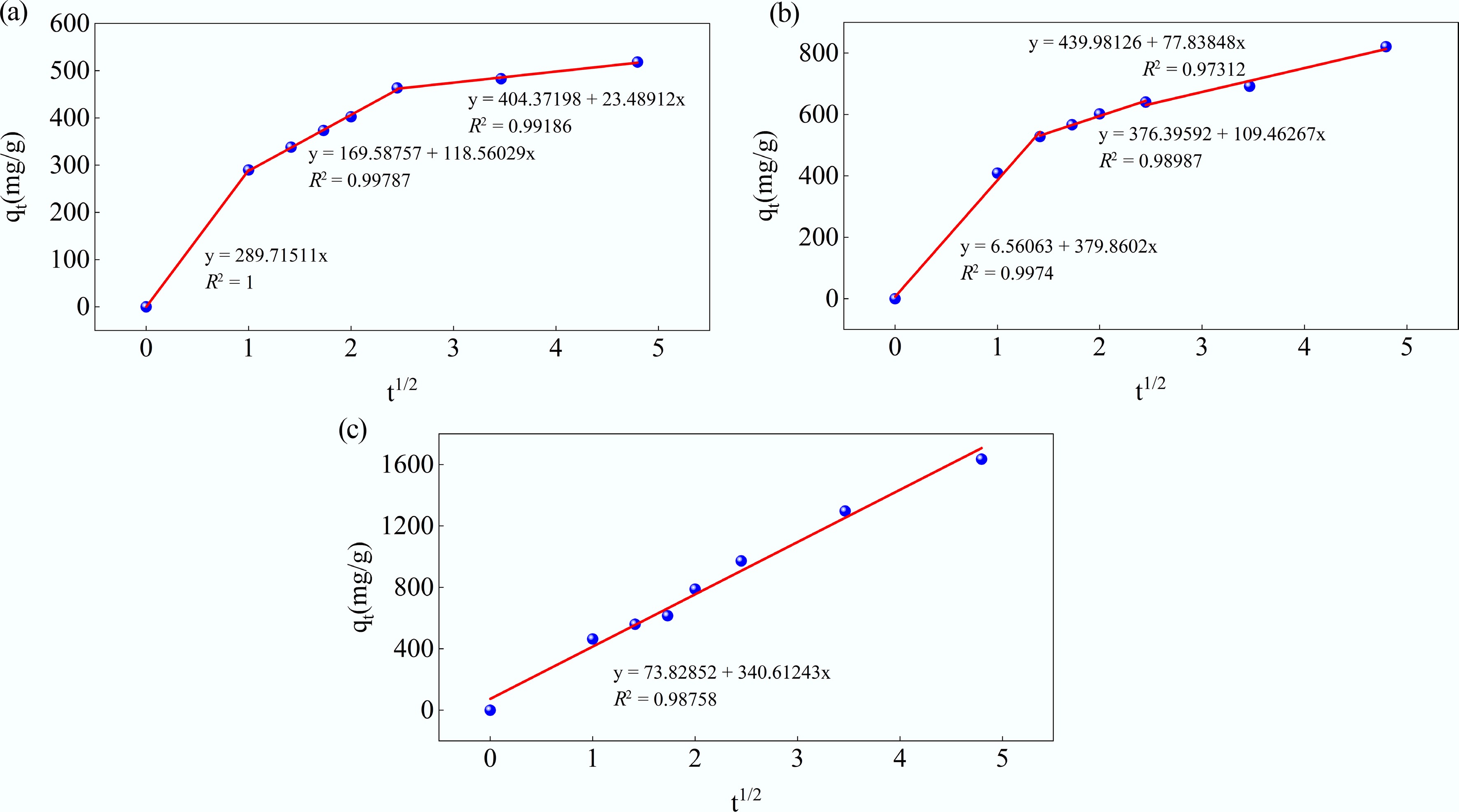
Figure 13.
Kinetic fits for MB adsorption on MAHC at (a) 24 °C, (b) 34 °C, and (c) 44 °C using the intraparticle diffusion model.
-
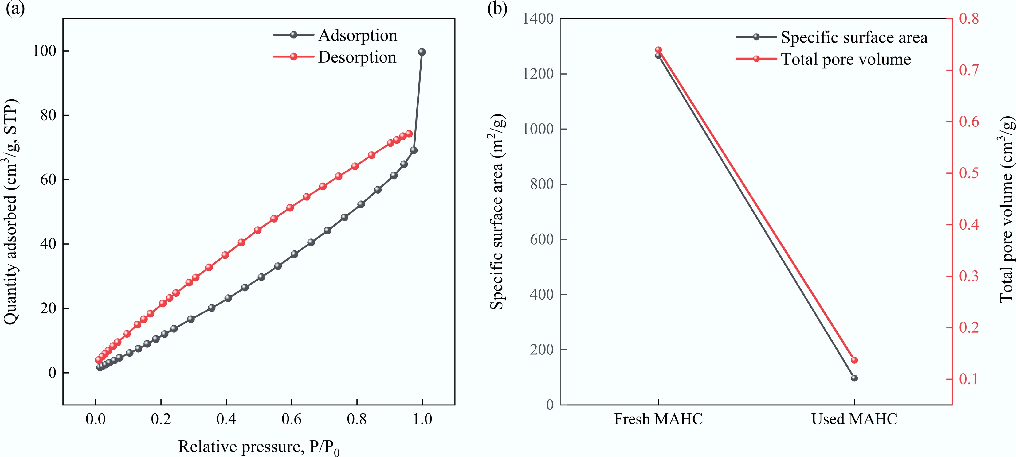
Figure 14.
(a) Adsorption/desorption isotherm of used MAHC, and (b) comparison of specific surface area and total pore volume between fresh MAHC and used MAHC.
-
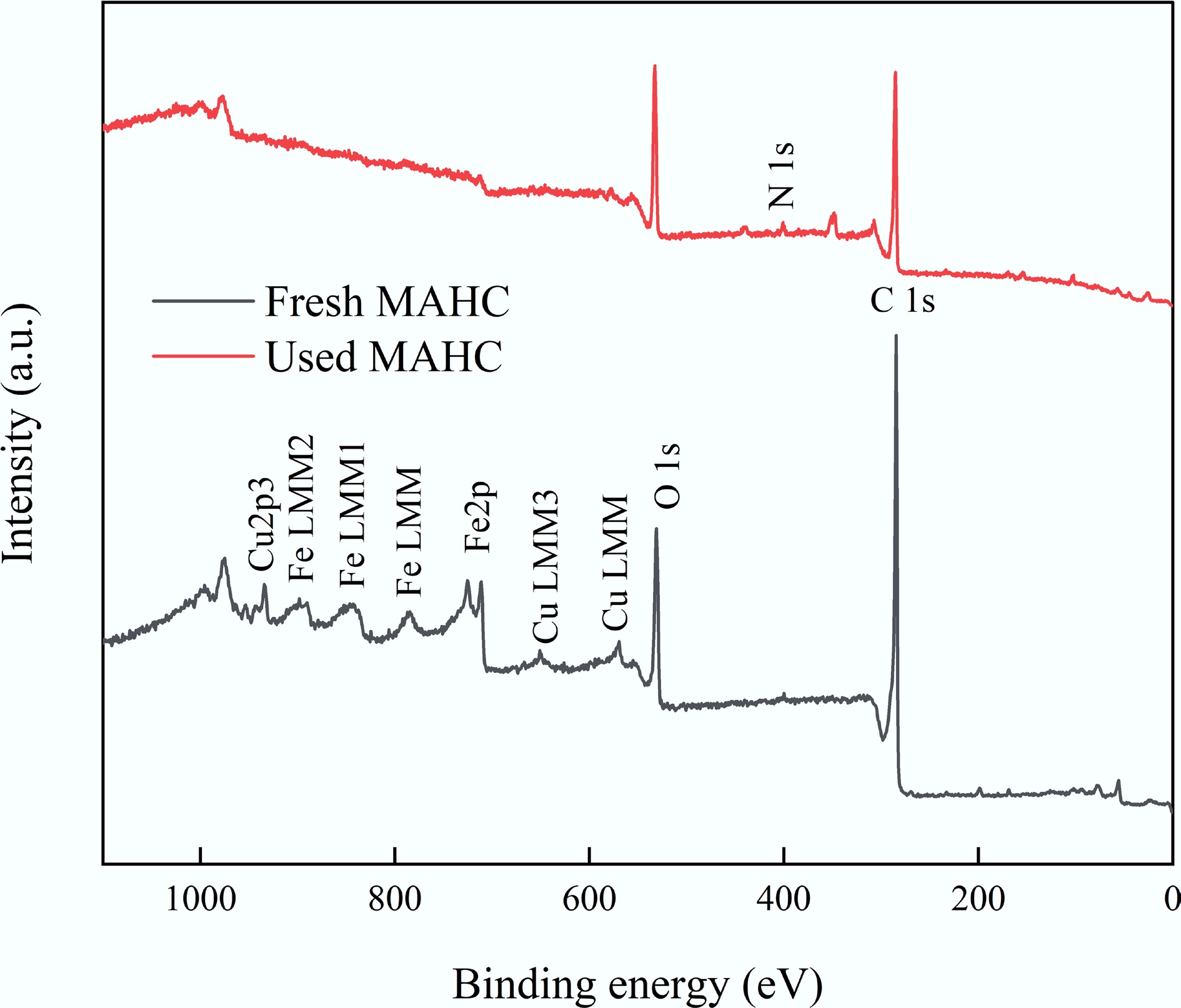
Figure 15.
XPS survey scan results of MAHC before and after MB adsorption.
-
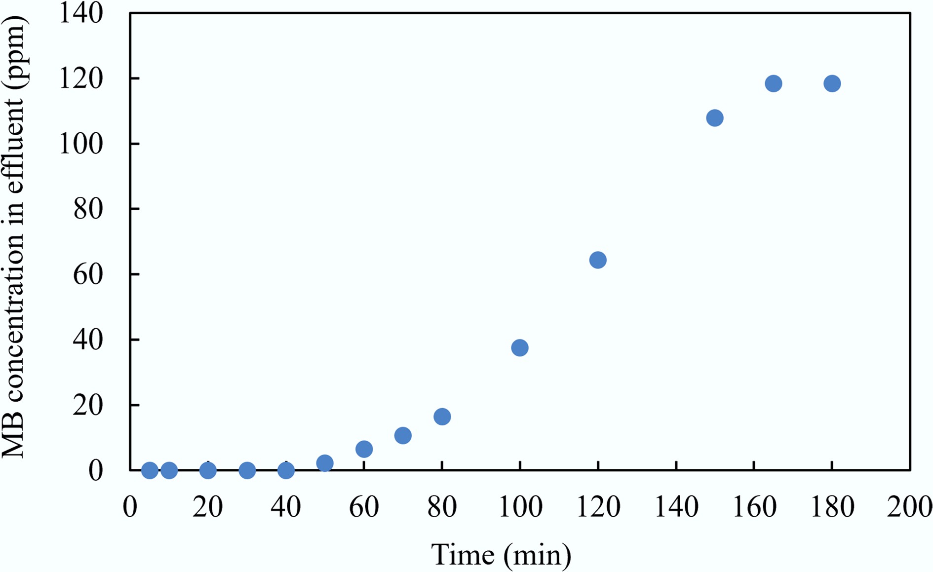
Figure 16.
Breakthrough curve of MAHC to treat the MB solution.
-
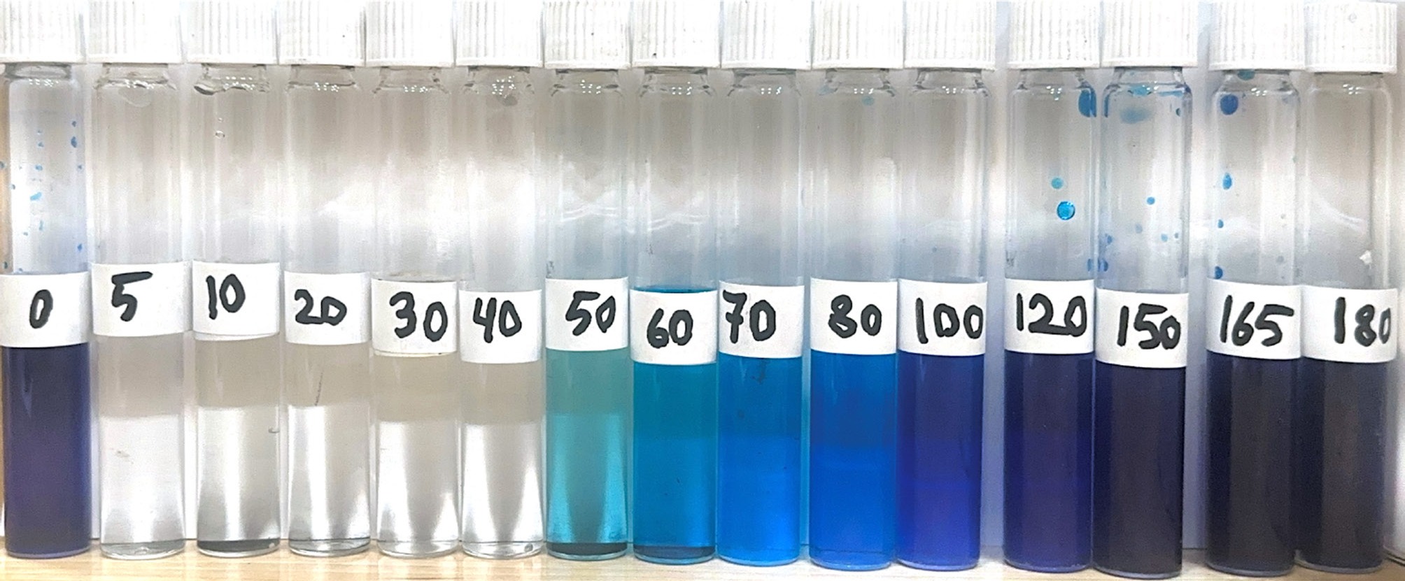
Figure 17.
MB adsorption experiment in a fixed bed column over 180 min.
-
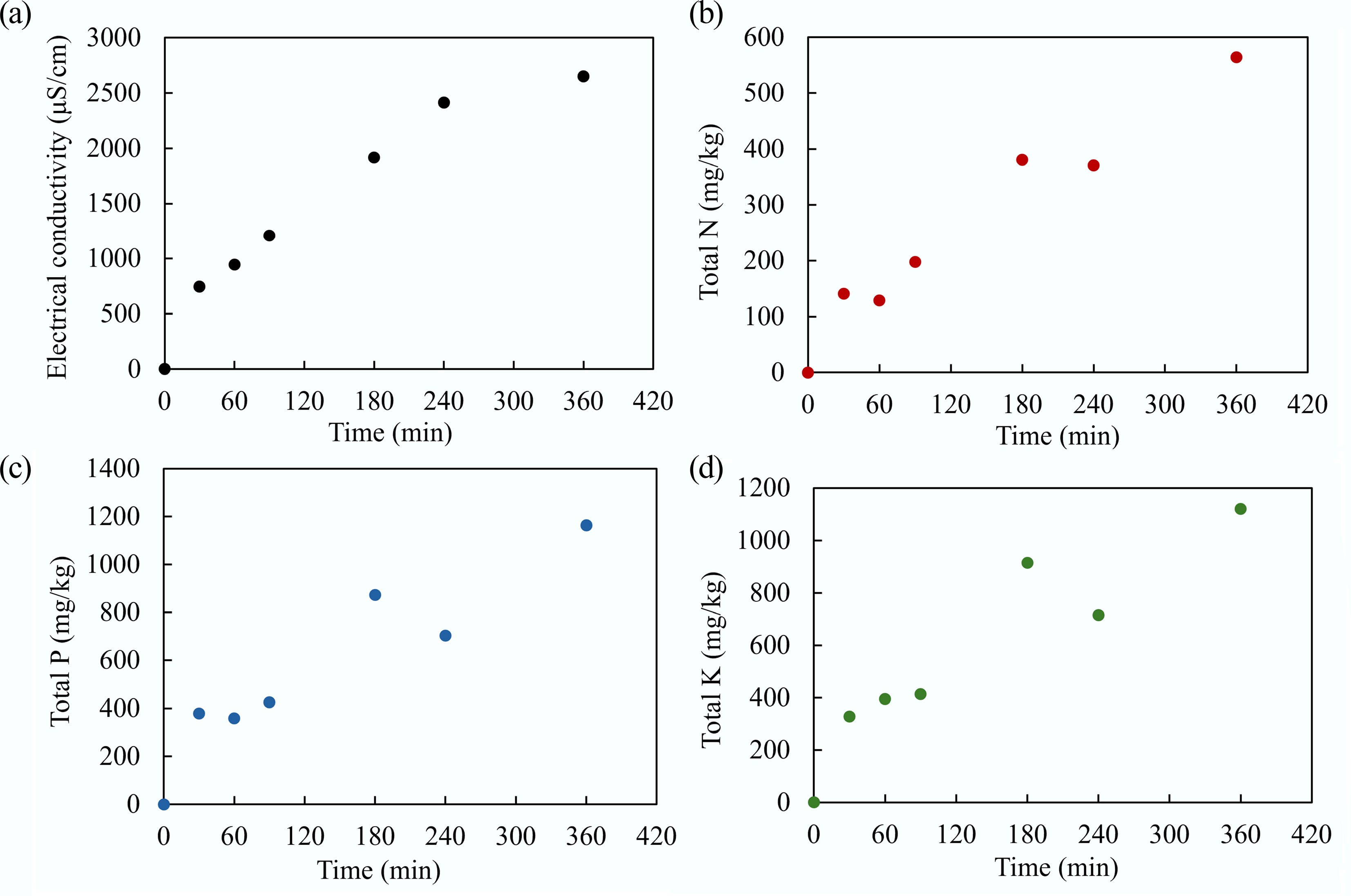
Figure 18.
(a) Electrical conductivity, and the concentration of (b) total N, (c) total P, and (d) total K in the effluent over 360 min.
-
Property Value Electrical conductivity (μs/cm) 2,961 Total nitrogen (mg/g) 588 Total phosphorus (mg/g) 1,219 Total potassium (mg/g) 1,269 Table 1.
Analysis of real wastewater provided by a local potato processing facility
-
C H O1 N S2 Ash3 Sawdust 47.76 5.90 44.34 n.d. n.d. 2.00 Hydrochar 53.45 3.28 38.18 n.d. n.d. 5.09 Activated hydrochar 78.42 2.72 7.88 0.28 n.d. 10.70 MAHC 79.13 1.26 12.23 0.22 n.d. 7.16 1 Oxygen content was estimated by difference. 2 n.d. represents not detectable. 3 Ash content was measured using thermal gravimetric analysis in air up to 900 °C and held at 900 °C for 30 min. Table 2.
Elemental composition of sawdust, hydrochar, activated hydrochar, and MAHC
-
Iodine number Value (mg/g) This study 612.3 Sludge-derived activated carbon using ZnCl2[36] 531.8 Sludge-derived activated carbon using KCl[36] 376.0 Sludge-derived activated carbon using ZnCl2 and H2SO4[36] 446.9 Sludge-derived activated carbon using ZnCl2 and KOH[36] 363.9 Sludge-derived activated carbon using KOH[36] 439.0 Acorn shell-derived activated carbon using ZnCl2[37] 37–1,209 Calgon carbon (powdered activated carbon) > 500 CS corporation (powdered activated carbon) 500–2,500 Table 3.
Iodine number of MAHC compared with the literature and commercial activated carbon
-
Isotherm model Parameter Values Langmuir qm (mg/g) 2,651.606 kL(L/mg) 0.005017 R2 0.66229 Freundlich 1/nf 0.81246 kf (mg/g)(L/mg)1/n 22.15648 R2 0.97576 Temkin bt 0.006205 kT (L/mg) 0.075853 R2 0.97114 Table 4.
Isotherm model parameters
-
T Pseudo-first-order Pseudo-second-order qe (mg/g) k1 (min−1) R2 qe (mg/g) k2 (min−1) R2 24 °C 299.8643 0.20532 0.86046 543.4783 0.001539 0.9992 34 °C 463.8448 0.85966 0.73901 854.7009 0.000724 0.9931 44 °C 1437.47 0.12354 0.98077 1968.206 9.39E-05 0.9779 Table 5.
Kinetic model fitting parameters for the pseudo-first-order and pseudo-second-order models
-
Temperature Stage Kp (mg/(g·min1/2)) C (mg/g) R2 24 °C First stage 289.7151 0 1 Second stage 118.5603 169.5876 0.99787 Third stage 23.48912 404.37198 0.99186 34 °C First stage 379.8602 6.56063 0.9974 Second stage 109.46267 376.3959 0.98987 Third stage 77.83848 439.9813 0.97312 44 °C First stage 340.61243 73.82852 0.98758 Table 6.
Kinetic model fitting parameters for the intraparticle diffusion model
Figures
(18)
Tables
(6)