-
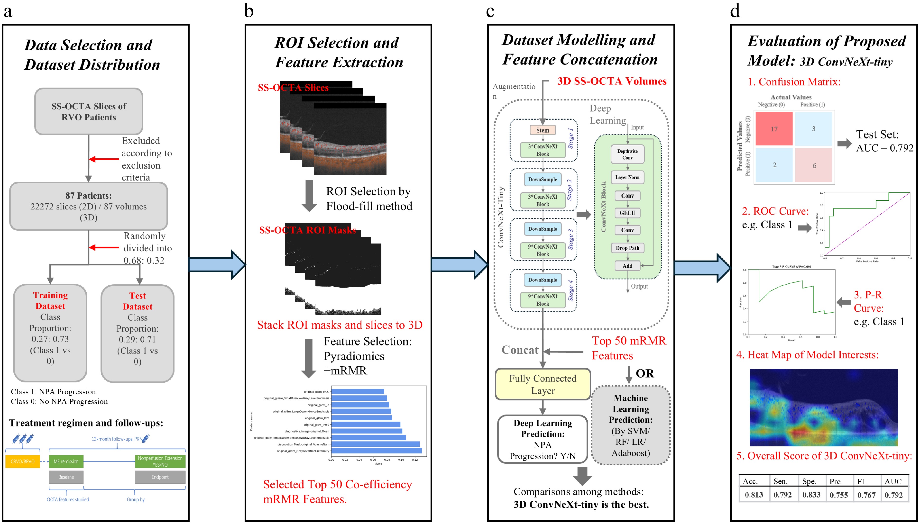
Figure 1.
The flow diagram of our proposed SS-OCTA-omics. (a) Indicates the screening method regarding the selection criteria of the clinical data and acquisition of original SS-OCTA images. The acquired dataset is divided into a training dataset and a test dataset at a ratio of 0.68:0.32. (b) Shows the Regions of interest (ROI) selection and feature selection. (c) Shows the integration of deep learning features with the selected radiomics features. (d) Shows the evaluation results together with an example heatmap visualization.
-
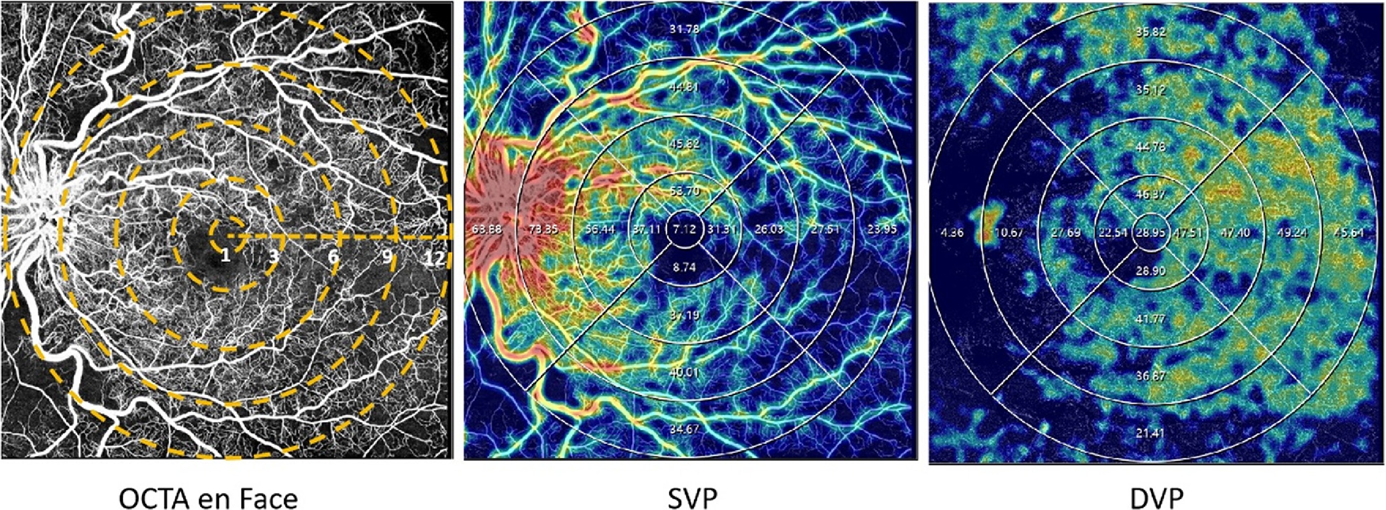
Figure 2.
Examples of quantitative measurement using OCTA. The left column represents the en face images (12 × 12 mm2) of color maps for vessel density. The middle and right columns represent the en face images of the corresponding layer of the SVP, and DVP of color perfusion maps. The vessel density of the SVP, and DVP were separately calculated in the whole area (diameter of 12 mm) and concentric rings with different radii (0–1,1–3, 3–6, 6–9, and 9–12 mm2). DVP refers to deep vascular plexus; SVP represents superficial vascular plexus.
-
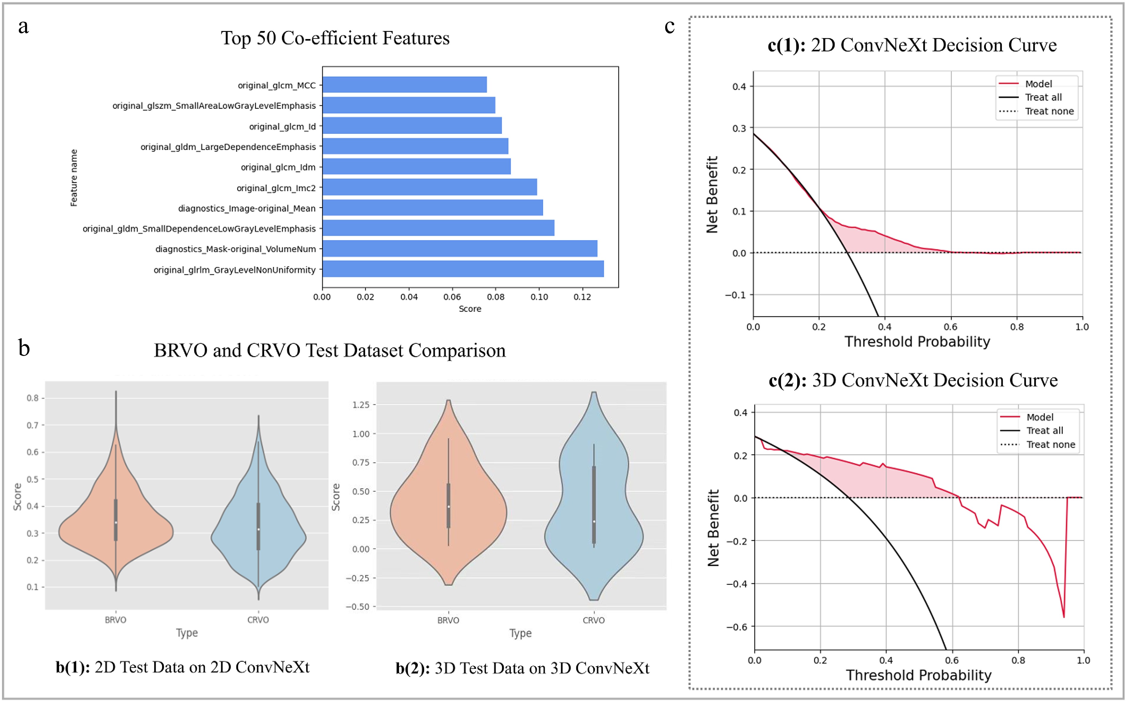
Figure 3.
SS-OCTA-omics model evaluation results and feature correlation plot. (a) Visualizes the top ten out of 50 radiomics features processed by mRMR. (b) Depicts the violin plots on external test dataset for the 2D and 3D ConvNeXt-tiny model with prediction confidence score distributions by performing the comparison of BRVO and CRVO types. (c) Shows the decision curves for the best 2D and 3D prediction models on an external test dataset.
-
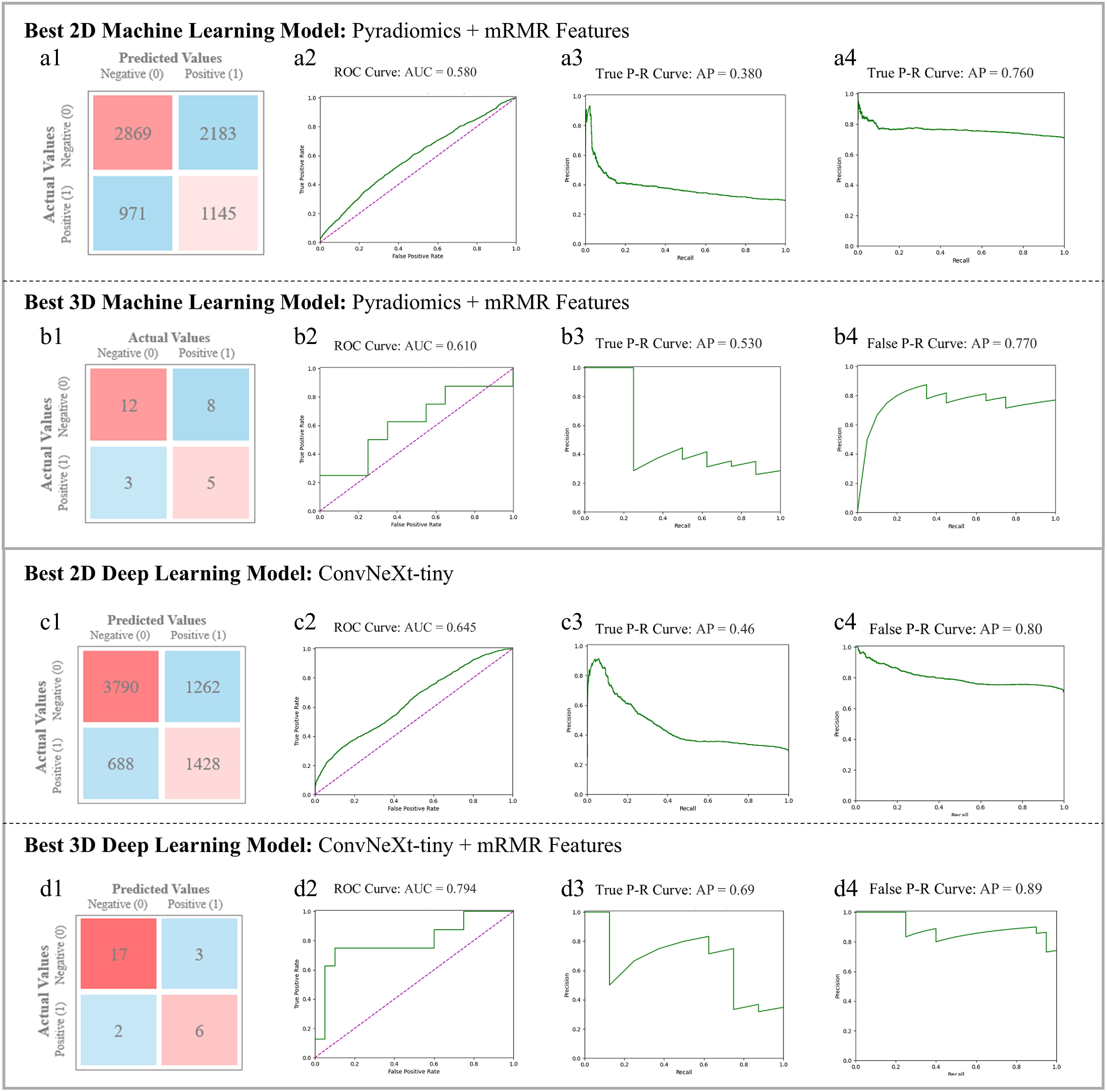
Figure 4.
Comparison of SVM with mRMR in (a) best 2D Machine Learning model (utilizing Pyradiomics and mRMR) and (b) best 3D Machine Learning model (utilizing Pyradiomics and mRMR). Each sub-figures (1)~(4) show the Confusion Matrix, ROC and class-based P-R curves. Radiomics-based mRMR features are classified by SVM. The Average Precision (AP) values refer to the area under the P-R curves. (c) Best 2D Deep Learning Model (ConvNeXt-tiny) figures, in which sub-figure (1)~(4) depict its visualization results; (d) 3D SS-OCTA-omics (utilized ConvNeXt-tiny and mRMR) figures, in which sub-figure (1)~(4) show its visualization results as the best 3D model.
-
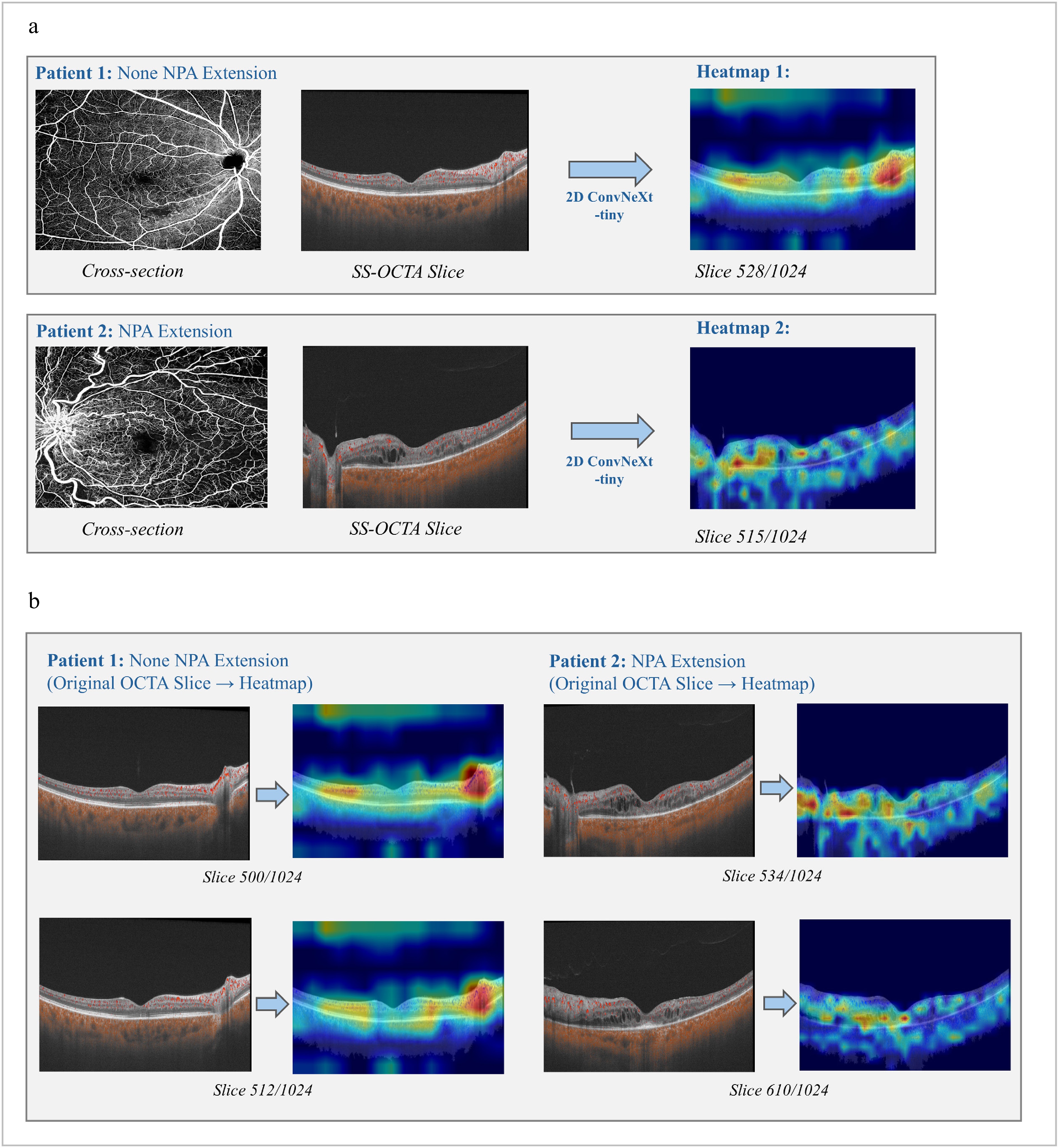
Figure 5.
Heatmaps generated by the best 2D model: ConvNeXt-tiny. (a) Comparisons between cross-section Angio-flow OCTA images and original SS-OCTA slices for both types of patient samples. (b) SS-OCTA original slices and its heatmaps for each type of patient with relatively high degree of confidences.
-
Characteristics Internal cohort External validation cohort Overall Stable Progressed p-value Overall Stable Progressed p-value Number of patients 87 63 24 109 58 51 Age (years) 65.17 (14.19) 64.83 (15.53) 66.08 (10.09) 0.714 66.35 (13.30) 66.17 (13.64) 66.55 (13.03) 0.782 Number of images 2D: 22272; 3D: 87 2D: 16128; 3D: 63 2D: 6144; 3D: 24 2D: 27904; 3D: 109 2D: 14848; 3D: 58 2D: 13056; 3D: 51 RVO duration (months) 9.91 (4.62) 10.06 (4.73) 9.50 (4.39) 0.614 10.11 (1.45) 10.00 (1.33) 10.24 (1.58) 0.326 IOP (mmHg) 14.84 (2.93) 14.81 (2.74) 14.92 (3.43) 0.875 14.75 (4.02) 14.66 (3.05) 14.84 (4.93) 0.640 DM (%) N/A N/A No 87 (100.00) 63 (100.00) 24 (100.00) 109 (100.00) 58 (100.00) 51 (100.00) Yes 0 0 0 0 0 0 Hypertension (%) 0.908 0.242 No 28 (32.18) 21 (33.33) 7 (29.17) 27 (24.77) 17 (29.31) 10 (19.61) Yes 59 (67.82) 42 (66.67) 17 (70.83) 82 (75.22) 41 (70.69) 41 (80.39) Hyperlipidemia (%) 1.000 0.198 No 74 (85.06) 54 (85.71) 20 (83.33) 73 (66.97) 42 (72.41) 31 (60.78) Yes 13 (14.94) 9 (14.29) 4 (16.67) 36 (33.03) 16 (27.59) 20 (39.22) BCVA, LogMAR 0.60 (0.38) 0.57 (0.36) 0.68 (0.44) 0.224 0.95 (0.66) 0.90 (0.57) 1.01 (0.76) 0.744 Disease (%) 0.031 0.387 BRVO 51 (58.62) 32 (50.79) 19 (79.17) 68 (62.39) 34 (58.62) 34 (66.67) CRVO 36 (41.38) 31 (49.21) 5 (20.83) 41 (37.61) 24 (41.38) 17 (33.33) Gender (%) 0.797 0.191 Female 47 (54.02) 33 (52.38) 14 (58.33) 50 (45.87) 30 (51.72) 20 (39.22) Male 40 (45.98) 30 (47.62) 10 (41.67) 59 (54.13) 28 (48.28) 31 (60.78) Baseline NPA(PD) 3.62 (1.37) 3.61 (1.46) 3.64 (1.10) 0.921 3.66 (1.15) 3.64 (1.15) 3.68 (1.16) 0.677 12 months NPA (PD) 4.36 (1.72) 4.01 (1.68) 5.29 (1.52) 0.002 4.65 (1.61) 3.93 (1.23) 5.47 (1.60) < 0.001 12 months ΔNPA (PD) 0.74 (0.70) 0.39 (0.37) 1.65 (0.55) < 0.001 0.99 (0.86) 0.29 (0.24) 1.79 (0.54) < 0.001 NPA Progression Total (n = 24) BRVO CRVO Total (n = 51) BRVO CRVO NPA (PD) 5.42 (1.57) 4.67 (0.33) 8.30 (0.83) < 0.001 5.74 (1.76) 4.57 (0.32) 8.09 (0.82) < 0.001 Time 6.58 (1.56) 6.84 (1.61) 5.60 (0.89) 0.090 6.08 (0.89) 6.32 (0.84) 5.59 (0.80) 0.004 ΔNPA (PD) 1.79 (0.62) 1.54 (0.27) 2.71 (0.71) 0.001 2.06 (0.73) 1.62 (0.23) 2.94 (0.58) < 0.001 * The results are presented in the format of mean (std). Abbreviation: BCVA: Best Corrected Visual Acuity; BRVO: Branch Retinal Vein Occlusion; CRVO: Central Retinal Vein Occlusion; DM: Diabetes Mellitus; IOP: Intraocular Pressure; NPA: Nonperfusion Area; RVO: Retinal Vein Occlusion; PD: Papillary Disc Area; ΔNPA: changes of NPA between follow-up visit and baseline. Table 1.
Demographics of enrolled patients.
-
Evaluation model Acc. Sen. Spe. Pre. F1. AUC. 2D mRMR + RF 0.610
(0.597−0.621)0.220
(0.208−0.233)0.760
(0.749−0.770)0.310
(0.298−0.323)0.230
(0.218−0.243)0.510
(0.498−0.522)2D mRMR + LR 0.540
(0.526−0.552)0.430
(0.417−0.442)0.590
(0.577−0.601)0.340
(0.327−0.352)0.330
(0.317−0.343)0.520
(0.508−0.531)2D mRMR + SVM 0.560
(0.546−0.572)0.640
(0.628−0.651)0.610
(0.598−0.621)0.450
(0.438−0.462)0.530
(0.517−0.542)0.580
(0.568−0.591)2D mRMR + Adaboost 0.570
(0.555−0.584)0.520
(0.504−0.535)0.680
(0.667−0.693)0.400
(0.385−0.415)0.390
(0.371−0.409)0.580
(0.565−0.595)2D ResNet 0.701
(0.689−0.712)0.524
(0.510−0.536)0.477
(0.464−0.489)0.686
(0.675−0.697)0.473
(0.460−0.485)0.621
(0.610−0.632)2D ViT 0.699
(0.688−0.710)0.524
(0.513−0.533)0.612
(0.601−0.623)0.648
(0.638−0.658)0.540
(0.536−0.555)0.638
(0.626−0.651)2D ConvNeXt-tiny 0.728
(0.717−0.738)0.573
(0.560−0.585)0.621
(0.609−0.633)0.675
(0.664−0.686)0.565
(0.552−0.577)0.645
(0.634−0.656)2D ConvNeXt-tiny + 3D mRMR 0.730
(0.718−0.741)0.552
(0.540−0.564)0.967
(0.955−0.979)0.681
(0.669−0.693)0.530
(0.508−0.551)0.552
(0.540−0.562)3D mRMR + RF 0.660
(0.459−0.828)0.170
(0.010−0.450)0.880
(0.676−0.973)0.330
(0.100−0.651)0.220
(0.080−0.480)0.520
(0.315−0.725)3D mRMR + LR 0.540
(0.345−0.727)0.430
(0.177−0.711)0.590
(0.329−0.816)0.340
(0.137−0.612)0.380
(0.181−0.580)0.520
(0.315−0.725)3D mRMR + SVM 0.610
(0.406−0.789)0.620
(0.316−0.861)0.600
(0.323−0.837)0.400
(0.191−0.640)0.480
(0.280−0.680)0.610
(0.405−0.815)3D mRMR + Adaboost 0.630
(0.424−0.806)0.540
(0.251−0.808)0.670
(0.384−0.882)0.390
(0.173−0.643)0.450
(0.255−0.645)0.600
(0.395−0.805)3D ResNet 0.688
(0.487−0.849)0.605
(0.333−0.837)0.750
(0.476−0.927)0.610
(0.360−0.820)0.614
(0.410−0.790)0.655
(0.450−0.860)3D ViT 0.706
(0.505−0.862)0.613
(0.340−0.842)0.740
(0.466−0.919)0.636
(0.380−0.840)0.619
(0.415−0.795)0.750
(0.560−0.940)3D ConvNeXt-tiny 0.750
(0.551−0.893)0.778
(0.501−0.950)0.722
(0.442−0.910)0.714
(0.450−0.900)0.745
(0.550−0.880)0.779
(0.594−0.963)3D ConvNeXt-tiny + 3D mRMR 0.821
(0.631−0.939)0.800
(0.519−0.957)0.833
(0.545−0.981)0.781
(0.484−0.945)0.788
(0.595−0.915)0.794
(0.613−0.975)* The 95% Confidence Interval values of proportion-based metrics were calculated using the Clopper-Pearson exact method, the Bootstrap method were used for calculating f1-score, the DeLong method was utilized for AUC. The methods highlighted in bold represent the best models among the compared 2D and 3D methods; the bolded data for each metric represents the best result point estimate of each metric. Table 2.
Comparisons among machine learning methods and deep learning methods on 2D and 3D dataset (with 95% confidence interval).
-
Evaluation model (external) Acc. Sen. Spe. Pre. F1. AUC. 2D ResNet 0.540
(0.533−0.546)0.430
(0.424−0.436)0.590
(0.584−0.596)0.340
(0.334−0.345)0.330
(0.322−0.337)0.520
(0.514−0.526)2D ViT 0.610
(0.604−0.616)0.220
(0.214−0.226)0.760
(0.755−0.765)0.310
(0.304−0.316)0.230
(0.221−0.237)0.510
(0.503−0.516)2D ConvNeXt−tiny 0.685
(0.679−0.690)0.545
(0.539−0.551)0.589
(0.583−0.595)0.638
(0.632−0.644)0.522
(0.515−0.528)0.612
(0.605−0.618)2D ConvNeXt+3D mRMR 0.678
(0.671−0.684)0.520
(0.514−0.526)0.680
(0.674−0.686)0.650
(0.644−0.656)0.528
(0.521−0.534)0.618
(0.612−0.624)3D ResNet 0.661
(0.564−0.749)0.569
(0.422−0.707)0.741
(0.603−0.850)0.659
(0.515−0.785)0.610
(0.512−0.701)0.621
(0.515−0.727)3D ViT 0.688
(0.592−0.773)0.608
(0.461−0.742)0.759
(0.624−0.865)0.689
(0.548−0.809)0.645
(0.548−0.734)0.701
(0.600−0.802)3D ConvNeXt-tiny 0.734
(0.641−0.814)0.706
(0.562−0.825)0.759
(0.624−0.865)0.720
(0.583−0.833)0.714
(0.621−0.796)0.749
(0.653−0.845)3D ConvNeXt+3D mRMR 0.771
(0.680−0.846)0.745
(0.604−0.857)0.793
(0.663−0.891)0.760
(0.628−0.864)0.753
(0.663−0.829)0.768
(0.674−0.862)* The 95% Confidence Interval values of proportion-based metrics were calculated using the Clopper-Pearson exact method, the Bootstrap method were used for calculating f1-score, the DeLong method was utilized for AUC. The methods highlighted in bold represent the best models among the compared 2D and 3D methods; the bolded data for each metric represents the best result point estimate of each metric. Table 3.
Comparisons among machine learning methods and deep learning methods on 2D/3D external validation datasets (with 95% confidence interval).
Figures
(5)
Tables
(3)