Back Article

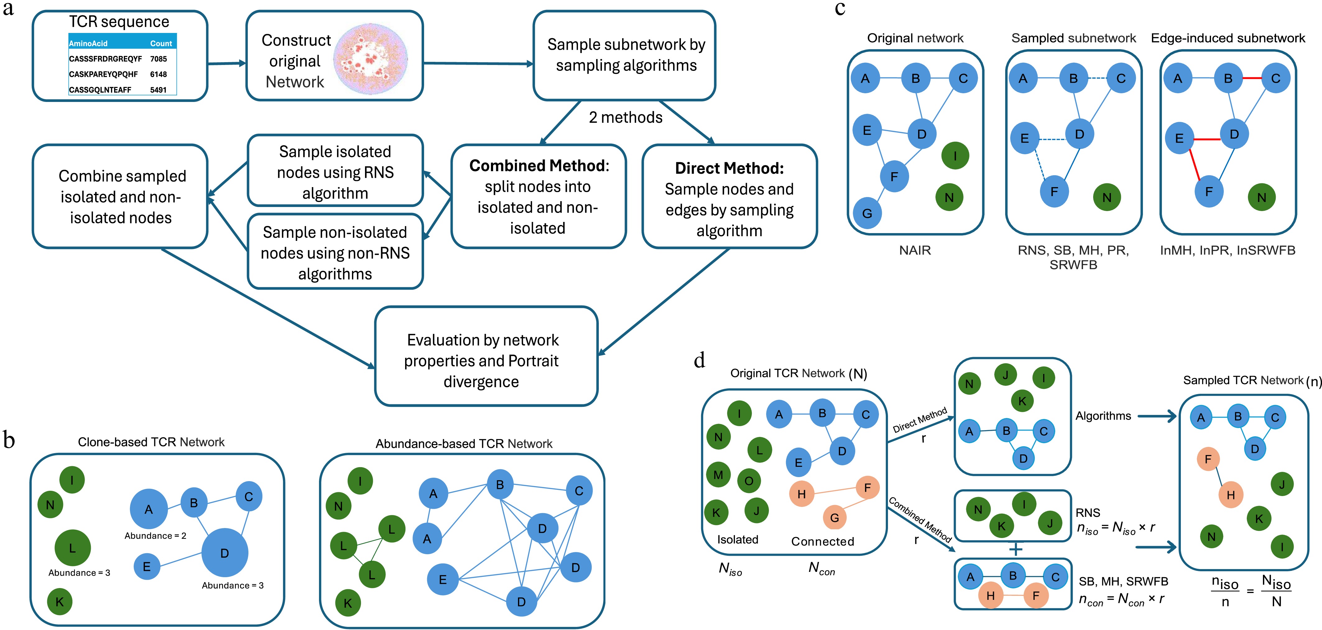
Figure 1. 

Schematic chart of subsampling approaches. (a) Analytic flow of network subsampling. (b) Clone-based and abundance-based TCR networks. Both networks are constructed by setting hamming distance between the TCR sequences equals to 1. Nodes in clone-based network correspond individual TCR sequences. In abundance-based network, nodes are expanded based on counts (abundance) of each unique TCR clone. (c) Pseudo examples of original network, and subnetwork by the original algorithm and the induced algorithm. (d) Illustration of the direct and combined strategies. In the direct method, a network is subsampled as a whole using one single algorithm. In the combined method, nodes are partitioned into isolated (N_iso) and connected (N_con) groups. To preserve network sparsity, both groups are subsampled at a consistent rate r, such that n_iso = N_iso × r, and n_con = N_con × r. This proportional scaling ensures the subnetwork's isolation rate matches the original n_iso/n = N_iso/N, preventing the edge-traversal bias of algorithms from artificially inflating connectivity. The subsampled results are then merged to form the final subnetwork.

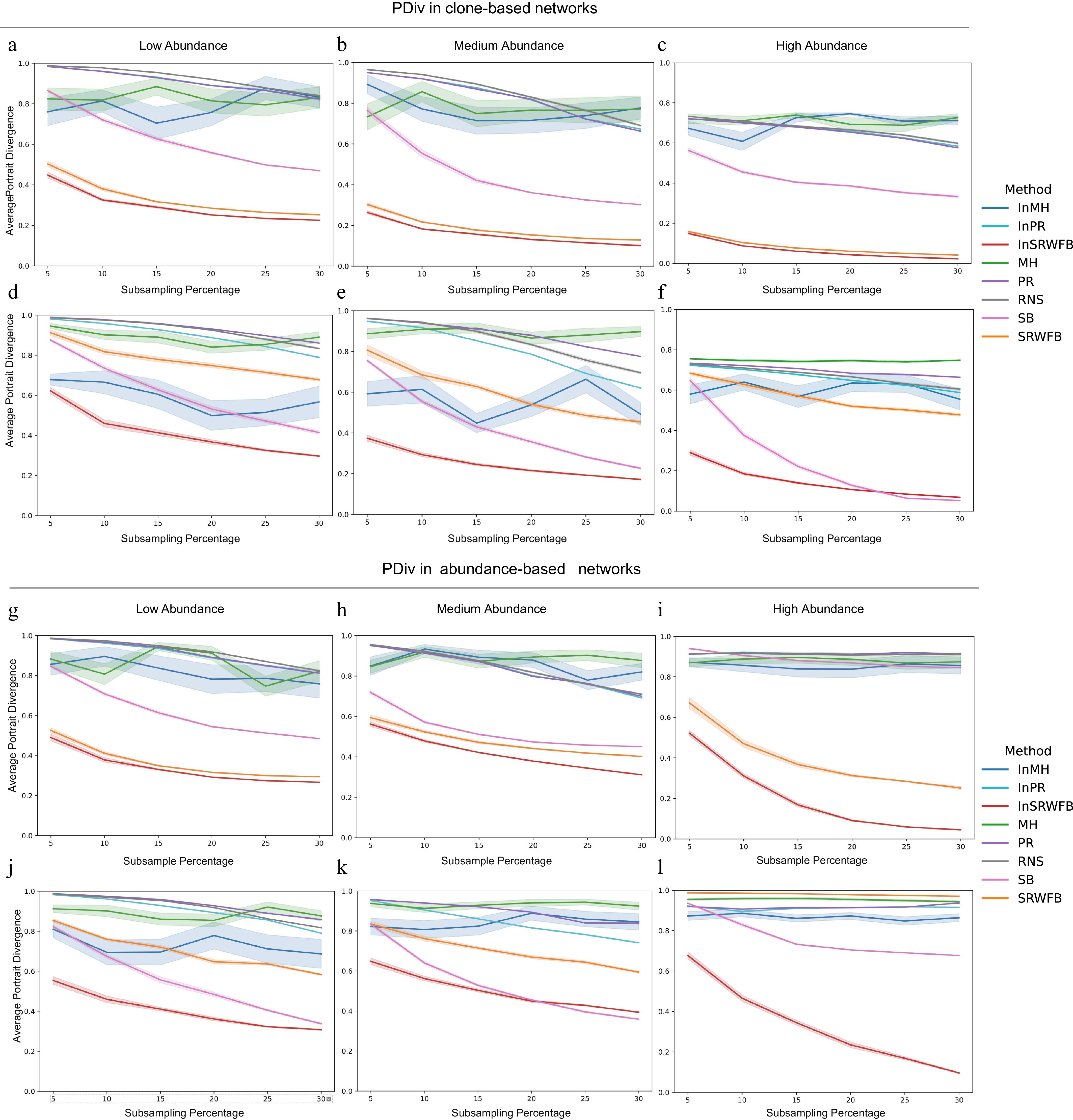
Figure 2. 

Average Portrait Divergence (PDiv) between the original network and the subnetwork. PDiv under the direct strategy for clone-based networks with (a) low, (b) medium, and (c) high abundance level. PDiv under the combined strategy for clone-based networks with (d) low, (e) medium, and (f) high (f) abundance level. PDiv under the direct strategy for abundance-based networks with (g) low, (h) medium, and (i) high abundance level. PDiv under the combined strategy for abundance-based networks with (j) low, (k) medium, and (l) high abundance level. Each curve represents PDiv change across different subsampling percentages (5% to 30%) for one of the subsampling algorithms, including Metropolis-Hastings (MH), PageRank (PR), Random Node Sampling (RNS), Snowball Sampling (SB), and SRWFB, and Induced Metropolis-Hastings (InMH), Induced PageRank (InPR), Induced Simple Random Walk with Fly Back (InSRWFB). For each subsampling percentage, 20 replicates were performed per method, and the lines represent the mean PD across replicates. Shaded areas indicate mean+/- standard error. Lower PD values indicate greater structural similarity between the subnetwork and original networks.

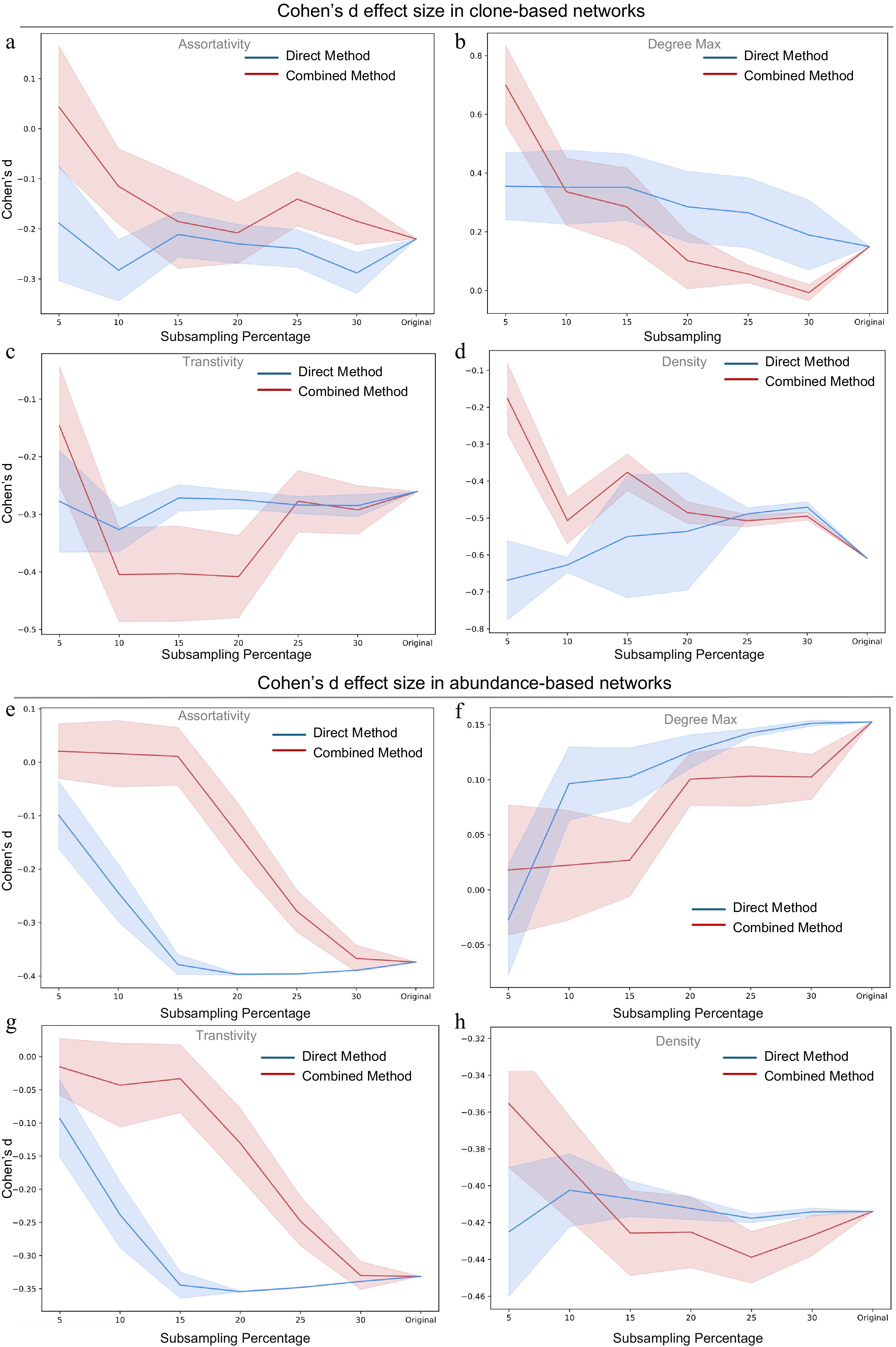
Figure 3. 

Cohen's d effect size of original network and subnetworks using Induced Simple Random Walk with Fly Back (InSRWFB) at different subsampling percentages (5% to 30%). Cohen's d effect size of (a) assortativity, (b) maximum degree, (c) transitivity, and (d) density by InSRWFB for clone-based networks. Cohen's d effect size of (e) assortativity, (f) maximum degree, (g) transitivity, and (h) density by InSRWFB for abundance-based networks. Cohen's d values were computed based on 11 patients at two time points to assess the magnitude and direction of change in the four network properties. For each patient and time point, 20 independent subsampling replicates were generated, and the resulting d values were averaged across replicates. Blue and red lines represent the direct and combined strategies, respectively. Shaded areas indicate mean +/− standard error.

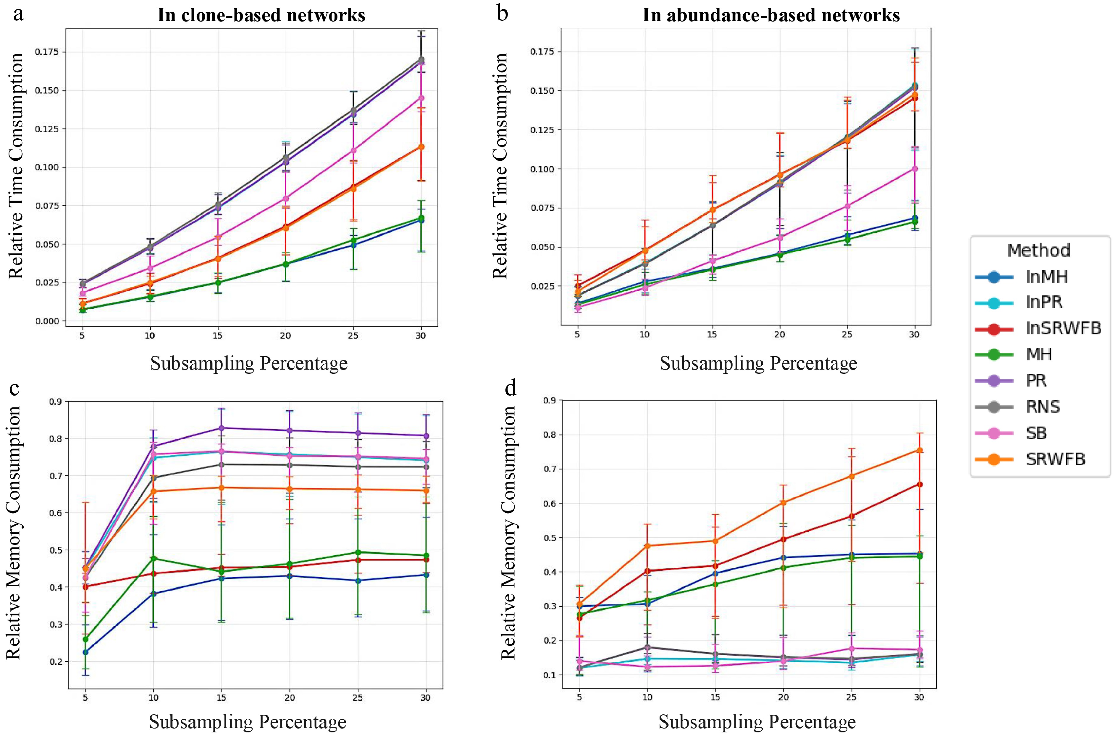
Figure 4. 

Computation Time and Memory Consumption Median relative runtime across 22 TCR samples for each subsampling method and percentage (5%–30%) in (a) clone-based, and (b) abundance-based networks. Median relative peak memory across the same samples in (c) clone-based, and (d) abundance-based networks. Error bars indicate the interquartile range (IQR; 25^th–75^th percentiles).