-
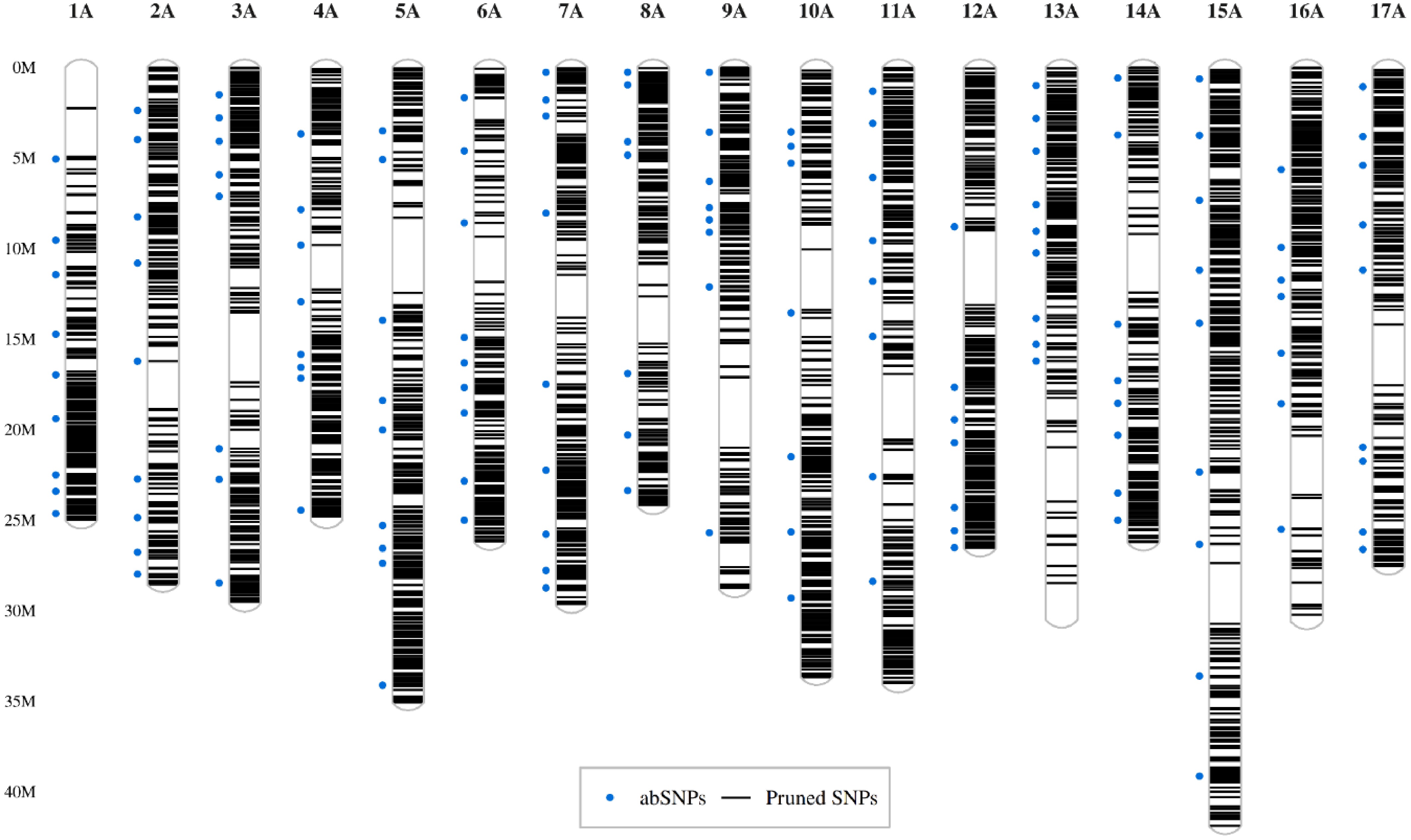
Figure 1.
Distribution of SNPs along the chromosomes. The set of 7,361 SNPs pruned by LD is displayed as black lines representing their positions along the chromosomes (y-axis). Blue dots on the left side of chromosomes indicate markers selected for amplicon sequencing.
-
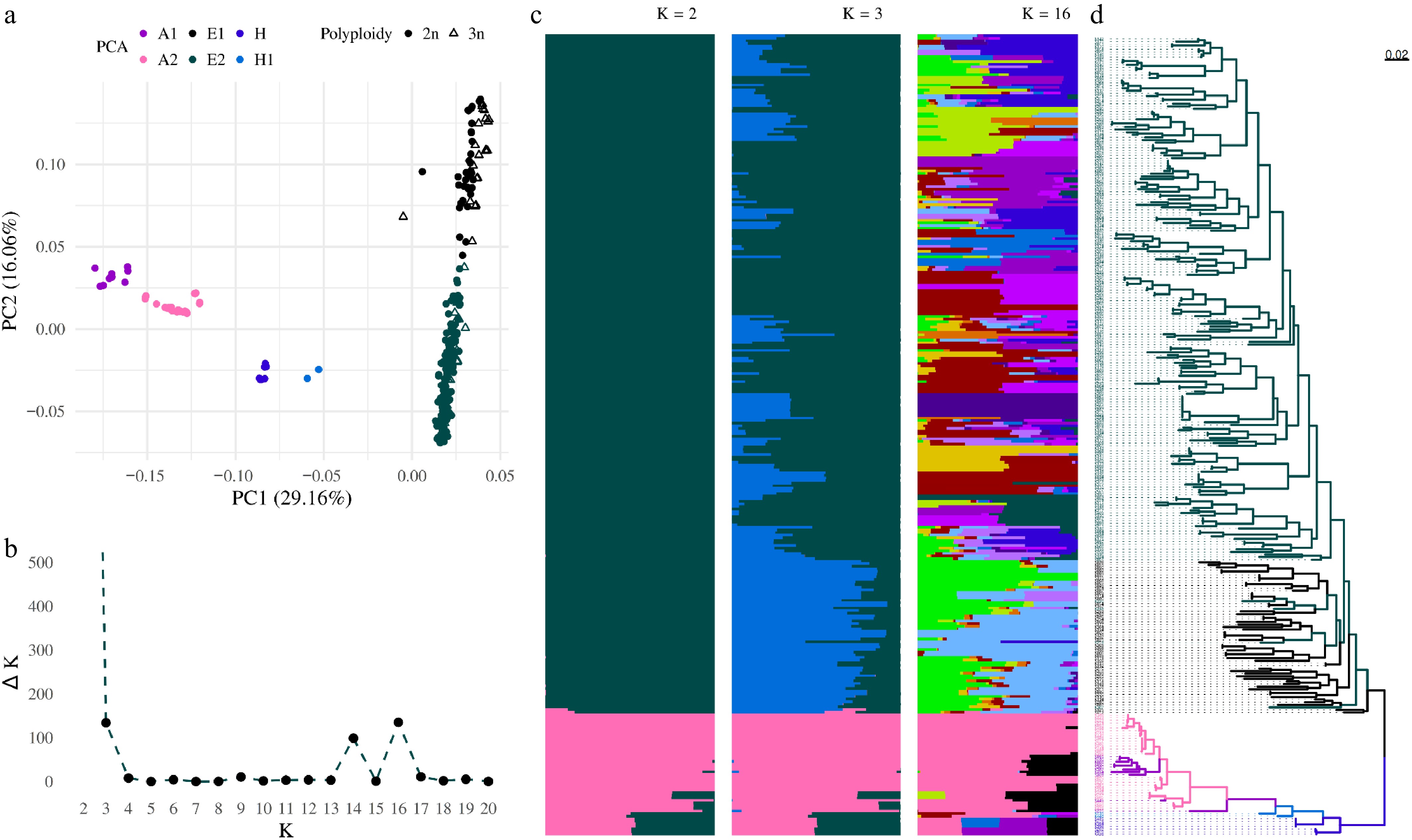
Figure 2.
Population structure analysis from pruned SNPs. All samples are divided according to principal component analysis into six groups. (a) Asian (A1, A2), European (E1, E2) accessions, and hybrids (H, H1) between Asian and European groups. (b) Plot of Delta K as a function of K within the range from 2 to 20. (c) Bar plots for K = 16, K = 3, and K = 2 illustrate the population structure described using a Bayesian approach. Each individual ordered according to the phylogenetic tree is represented by a horizontal line, with each color representing one of the inferred clusters. (d) The phylogenetic tree rooted at the midpoint was constructed using the SNPhylo pipeline. Accessions are colored according to the PCA color scheme.
-
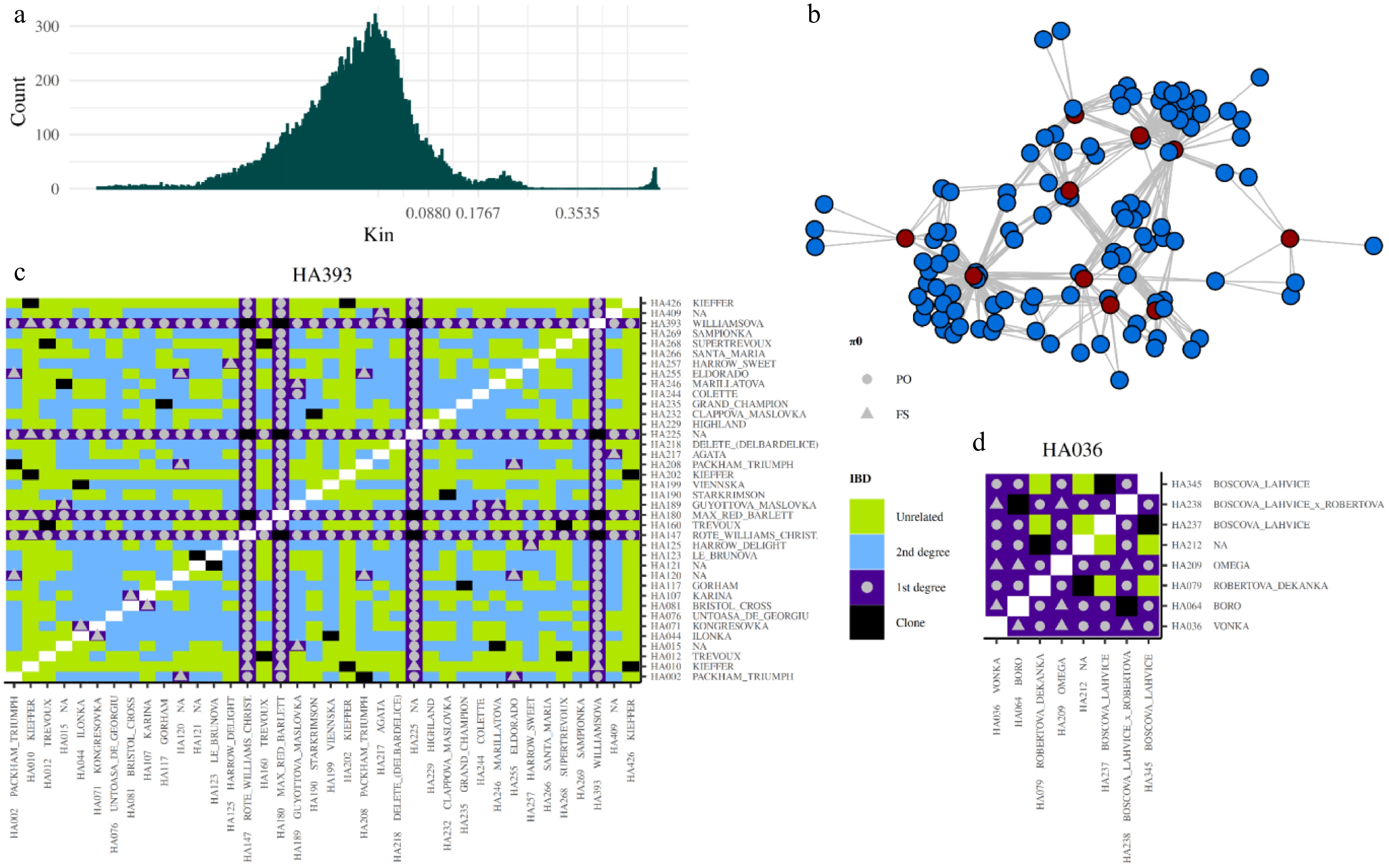
Figure 3.
Relationships defined using pairwise IBD coefficients. (a) Histogram showing the distribution of kinship coefficient values (x-axis) and their counts (y-axis) in diploid samples. The histogram is zoomed into the window of –0.5 to 0.5, with breaks representing different relationship categories: clone (> 0.3535), first-degree (> 0.1768–0.3535), second-degree (0.0880–0.1768), and unrelated (< 0.0880). (b) Network of first-degree relationships among donor accessions (red dots), with their offspring represented by blue dots. Lines connect nodes that share first-degree relationships, with kinship coefficients ranging from 0.1768 to 0.3535. (c) First-degree relationships with 'Williamsova', and (d) first-degree relationships with 'Vonka', along with the relationships of all filtered samples. The color of each tile in the heatmap represents the strength of the relationship, based on the kinship coefficient. Symbols in all first-degree relationships indicate whether the relationship is PO (parent-offspring) or FS (full-sibling), based on the π0.
-
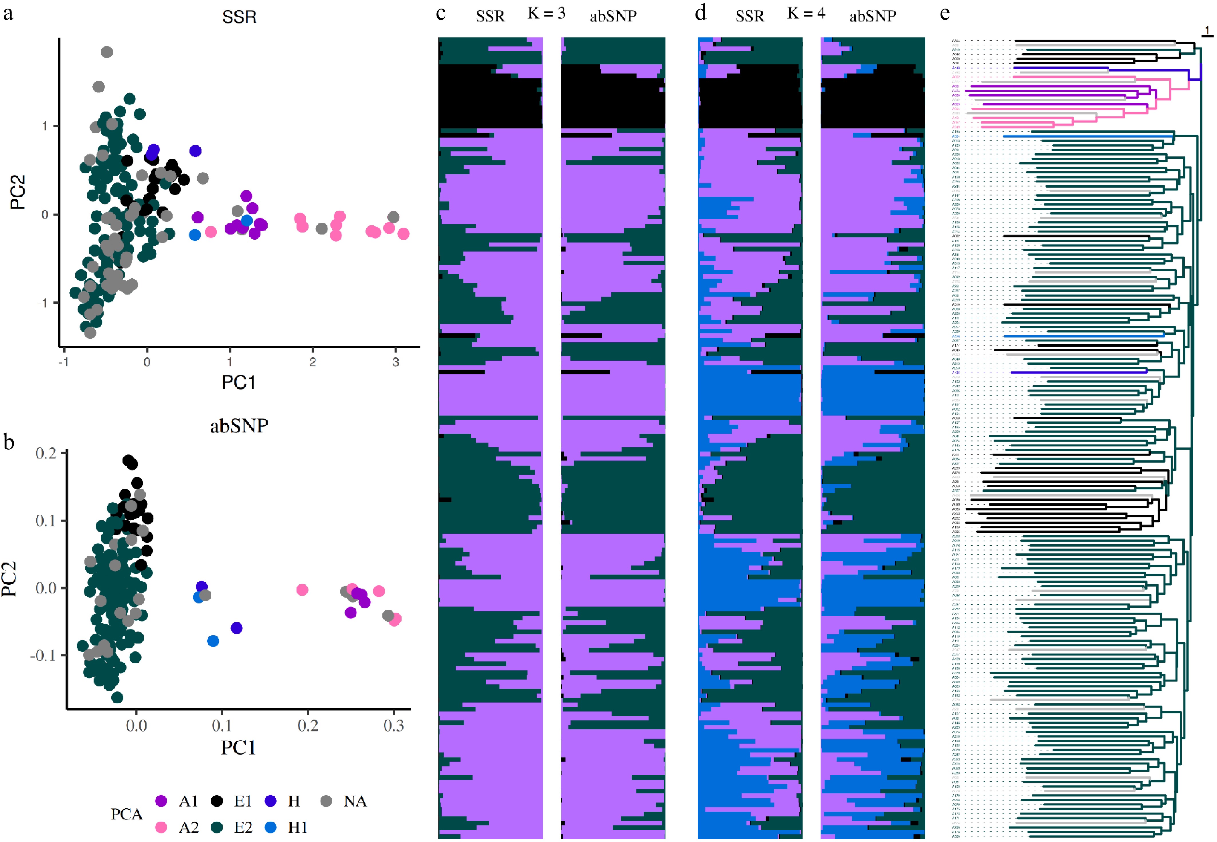
Figure 4.
Population structure analysis using markers. Principal component analysis (PCA) based on (a) SSR, and (b) amplicon-based SNP markers. Dots represent individual accessions and are colored according to their group membership, as defined by ddRAD analysis, (e) consistent with the phylogenetic tree generated from SSR markers. Bar plots, ordered according to the phylogenetic tree, illustrate population structure inferred using a Bayesian approach with SSR and abSNP markers for (c) K = 3, and (d) K = 4, with each cluster represented by a distinct color.
-
SSR marker Chromosome Motif Source of the SSR marker TsuENH003_a 1 (TC)n [49] CH02f06_a 2 (TG)n(AG)n [50] NB109a_a 3 (AG)n [51] NZ05g8_a 4 (GA)n [52] CH05e06_a 5 (AG)n [50] CH05a05_a 6 (AG)n [50] CH04e05_a 7 (GA)n [50] CH01h10_a 8 (TC)n [50] NB106a_a 9 (AG)n [51] CH02b03b_a 10 (TC)n [50] NB105a_a 11 (AG)nAT(AG)n [51] CH01d09_a 12 (GA)n [50] NH021a_a 13 (AG)n [51] CH05d03 14 (AG)n [50] CH02d11_a 15 (AG)n [53] CH05c06 16 (TC)n [50] GD96_a 17 (TC)n [54] The suffix '_a' in the marker name indicates that at least one primer used for amplification was designed at a position different from the original, i.e., the allele length amplified by the original primers differs from the length of the same allele amplified according to this study. However, both represent amplification of the same polymorphic locus within the genome. Table 1.
List of markers used for pear genotyping.
-
Relationship Kin Kin observed and set up (bold) Marking Kin π0 π0 observed (bold) and set up Marking π0 Monozygotes/clone > 0.3535 > 0.4654 and > 0.3535 Clone < 0.1 < 0.0003 Parent-offspring (PO) 0.3535– 0.1768 0.2604–0.1816 and 0.3535–0.1768 1st degree < 0.1 0.0022–0.0064 and 0–0.0064 PO Full-siblings (FS) 0.1–0.365 0.0064–0.1 FS 2nd degree 0.1768–0.088 Unrelated < 0.088 Observed Kin values were defined from documented relationships in our collection (Supplementary Data S2, Kin test). The Kin threshold was determined based on the correlation between observed values and the ranges defined by Manichaikul et al.[45]. The setup π0 thresholds were established based on observed data. Table 2.
Thresholds and observed values for genetic relationship inference.
Figures
(4)
Tables
(2)