Back Article

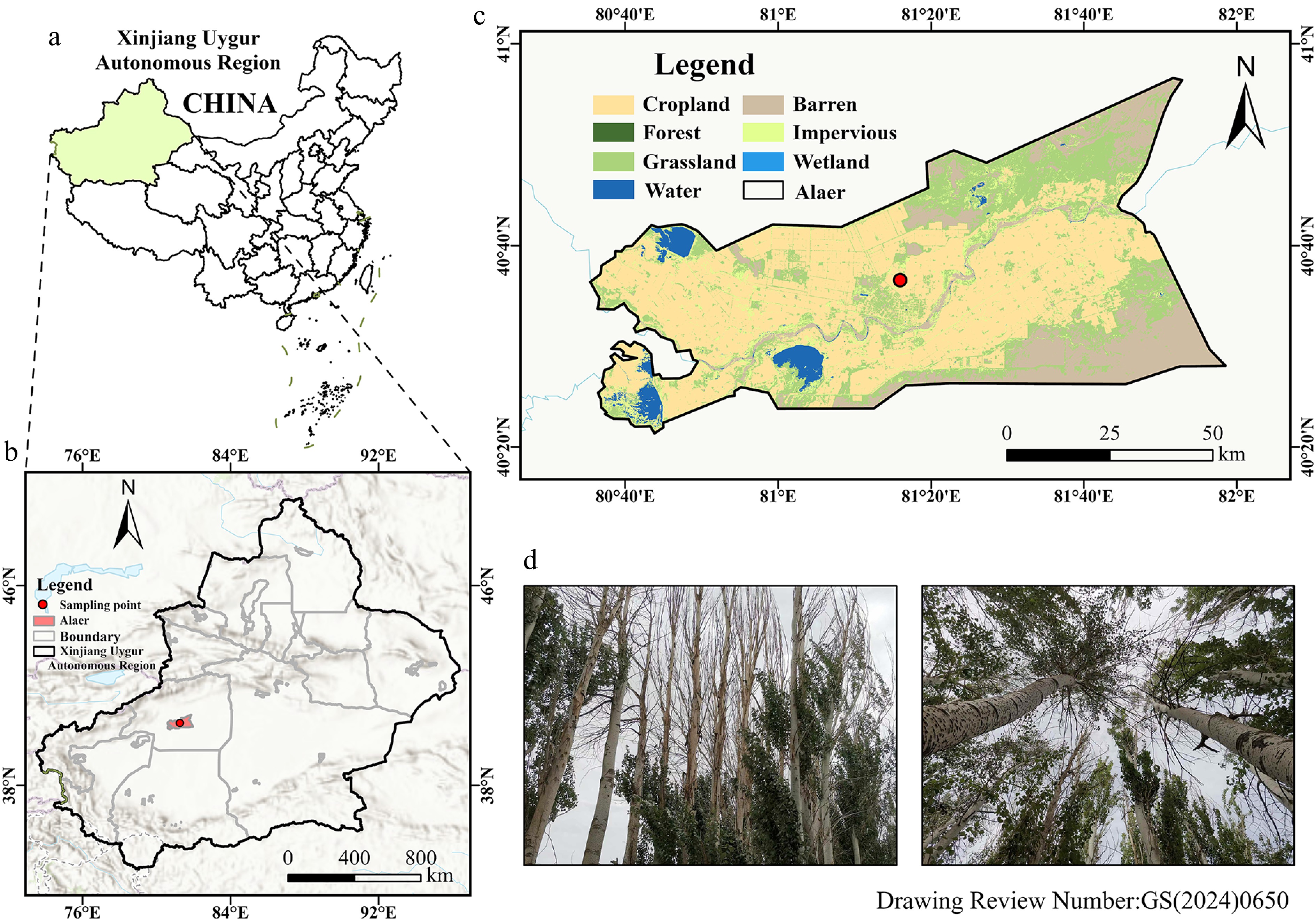
Figure 1. 

Map of the study area. (a) Location of the Xinjiang Uygur Autonomous Region in China. (b) Detailed location of Alar City in Aksu Prefecture, with the red dot indicating the specific study site. (c) Land use classification in Alar City, where dark green denotes forested regions and brown indicates agricultural land, both featuring farmland protection forests established to combat wind erosion and desertification. (d) Photograph showing farmland shelterbelts with poplars exhibiting varying degrees of decline. Base maps (a–c): https://cloudcenter.tianditu.gov.cn/administrativeDivision.

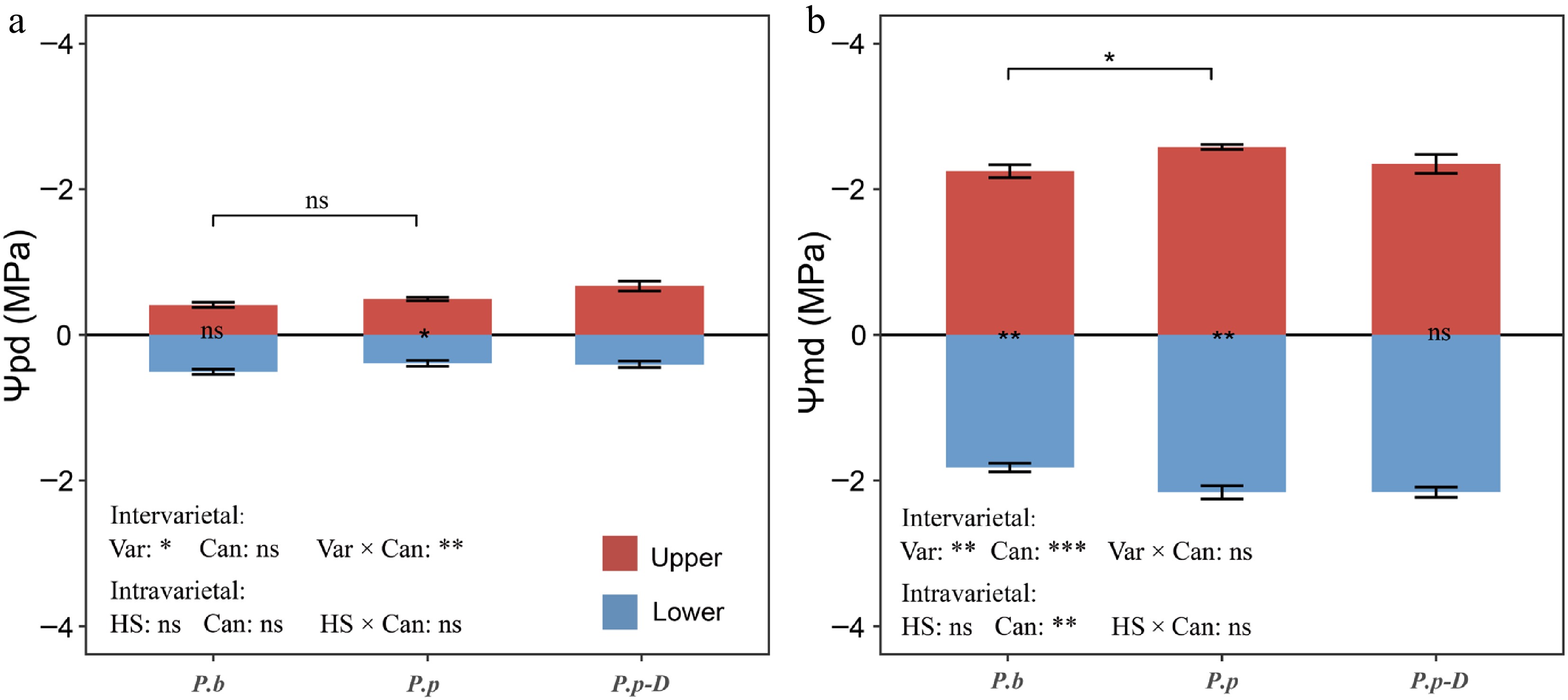
Figure 2. 

Variations in (a) Ψ_pd (predawn leaf water potential), and (b) Ψ_md (midday leaf water potential) across different comparisons: intervarietal (P.b vs P.p), intravarietal (P.p vs declining P.p-D), and between upper and lower canopy layers within each group. The effects of variety (or health status) and canopy position were assessed using two-way ANOVA. In the panel annotations, bracketed labels show between-group differences; bar-side labels show within-group canopy differences. 'Var' denotes variety, 'HS' denotes health status, 'Can' denotes canopy position, and 'Var × Can/HS × Can' denotes their respective interactions. 'ns' indicates no significant difference; asterisks indicate significant differences (* p < 0.05, ** p < 0.01, *** p < 0.001). Data are means ± SE (n = 6).

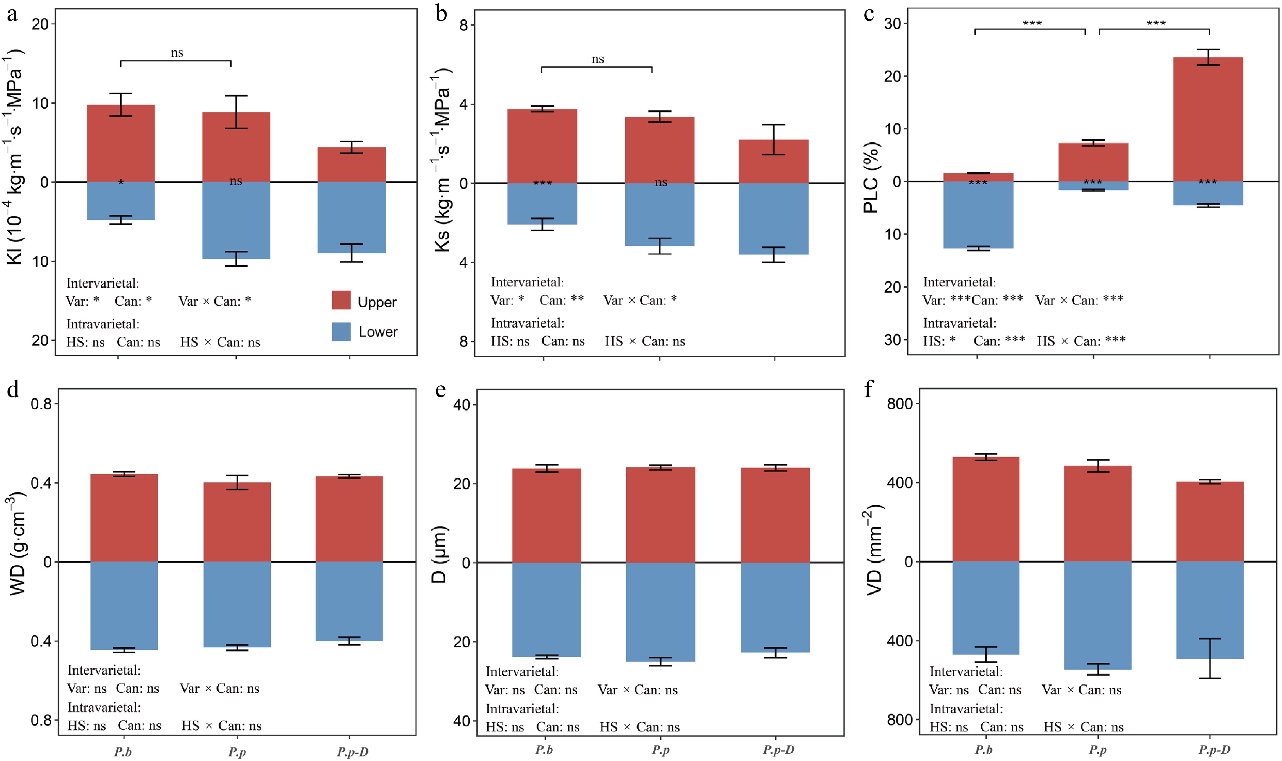
Figure 3. 

Variations in (a) K₁ (leaf-specific hydraulic conductivity), (b) K_s (sapwood-specific hydraulic conductivity), (c) PLC (percent loss of hydraulic conductivity), (d) WD (wood density), (e) D (mean vessel diameter), and (f) VD (vessel density) across different comparison groups: intervarietal (P.b vs P.p), intravarietal (healthy P.p vs declining P.p-D), and between upper and lower canopy positions within each group. The effects of variety (or health status) and canopy position were assessed using two-way ANOVA. Bracketed labels show between-group differences; bar-side labels show within-group canopy differences. 'ns' indicates no significant difference; asterisks indicate significance levels (* p < 0.05, ** p < 0.01, *** p < 0.001). Data are means ± SE (n = 6).

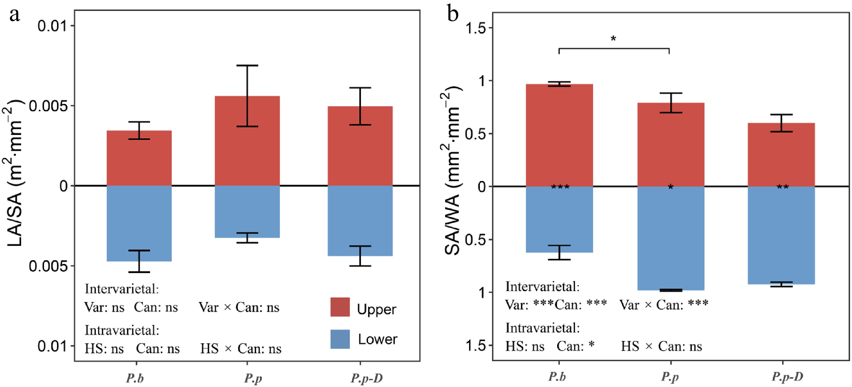
Figure 4. 

Variations in (a) LA/SA (leaf area to sapwood area ratio), an indicator of hydraulic supply–transpiration balance, and (b) SA/WA (sapwood area to whole cross-sectional wood area ratio), an indicator of functional xylem proportion, across different comparison groups: intervarietal (P.b vs P.p), intravarietal (healthy P.p vs declining P.p-D), and between upper and lower canopy positions within each group. The effects of variety (or health status) and canopy position were evaluated using two-way ANOVA. Bracketed labels show between-group differences; bar-side labels show within-group canopy differences. 'ns' indicates no significant difference; asterisks indicate significance levels (* p < 0.05, ** p < 0.01, *** p < 0.001). Data are means ± SE (n = 6).

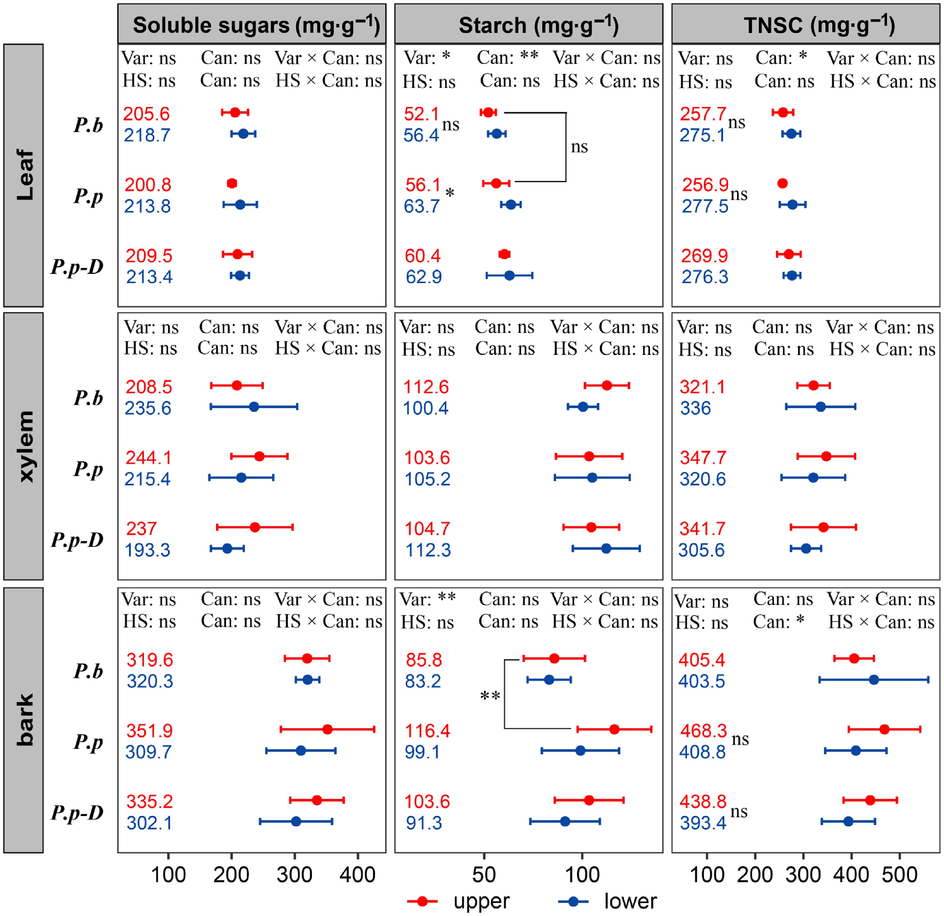
Figure 5. 

Variations in soluble sugars, starch, and total NSC in leaves, stems, and bark across different comparison groups: intervarietal (P.b vs P.p), intravarietal (healthy P.p vs declining P.p-D), and between upper and lower canopy positions within each group. The effects of variety (or health status) and canopy position were evaluated using two-way ANOVA. Bracketed labels show between-group differences; bar-side labels show within-group canopy differences. 'ns' marks non-significant differences; asterisks indicate significant differences (* p < 0.05, ** p < 0.01, *** p < 0.001). Data are means ± SE (n = 6).

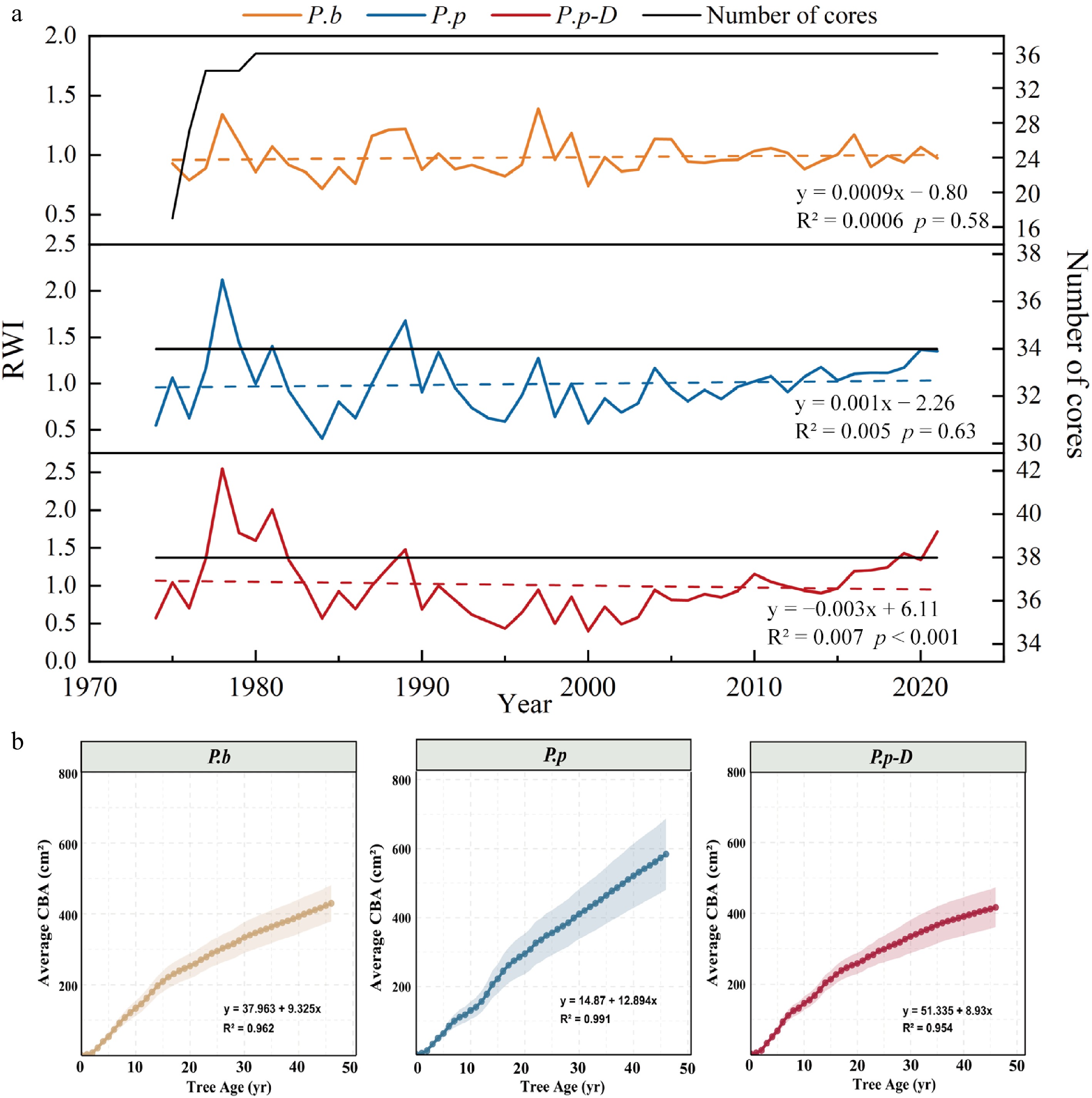
Figure 6. 

(a) Standardized tree-ring width index (RWI) chronologies for the three poplar groups. The black line indicates the number of cores available each year (right axis). (b) Average cumulative basal area increment (CBA) in relation to tree age for P.b, healthy P.p, and declining P.p-D. Shaded areas represent 95% confidence intervals, and solid lines represent regressions describing long-term growth trends.