-
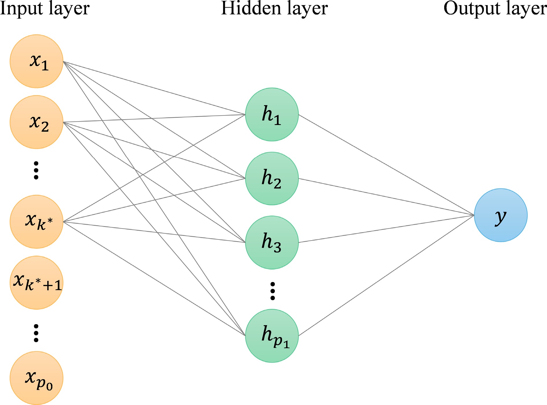
Figure 1.
The architecture of a one-hidden-layer neural network derived using the group
$ \ell_0 $ $ {x_{k^*+1}, \cdots , x_{p_0}} $ $ (k^*+1) $ $ p_0 $ $ {\bf{W}}_1 $ $ \ell_0 $ -
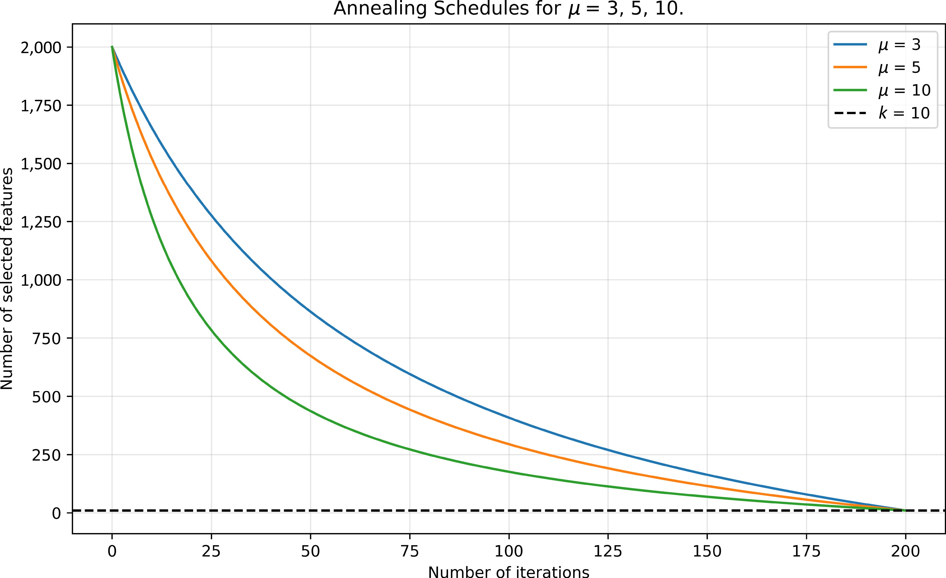
Figure 2.
Annealing schedule for p0 = 2,000, k = 10, Niter = 200, and multiple annealing parameters
$ \mu $ -
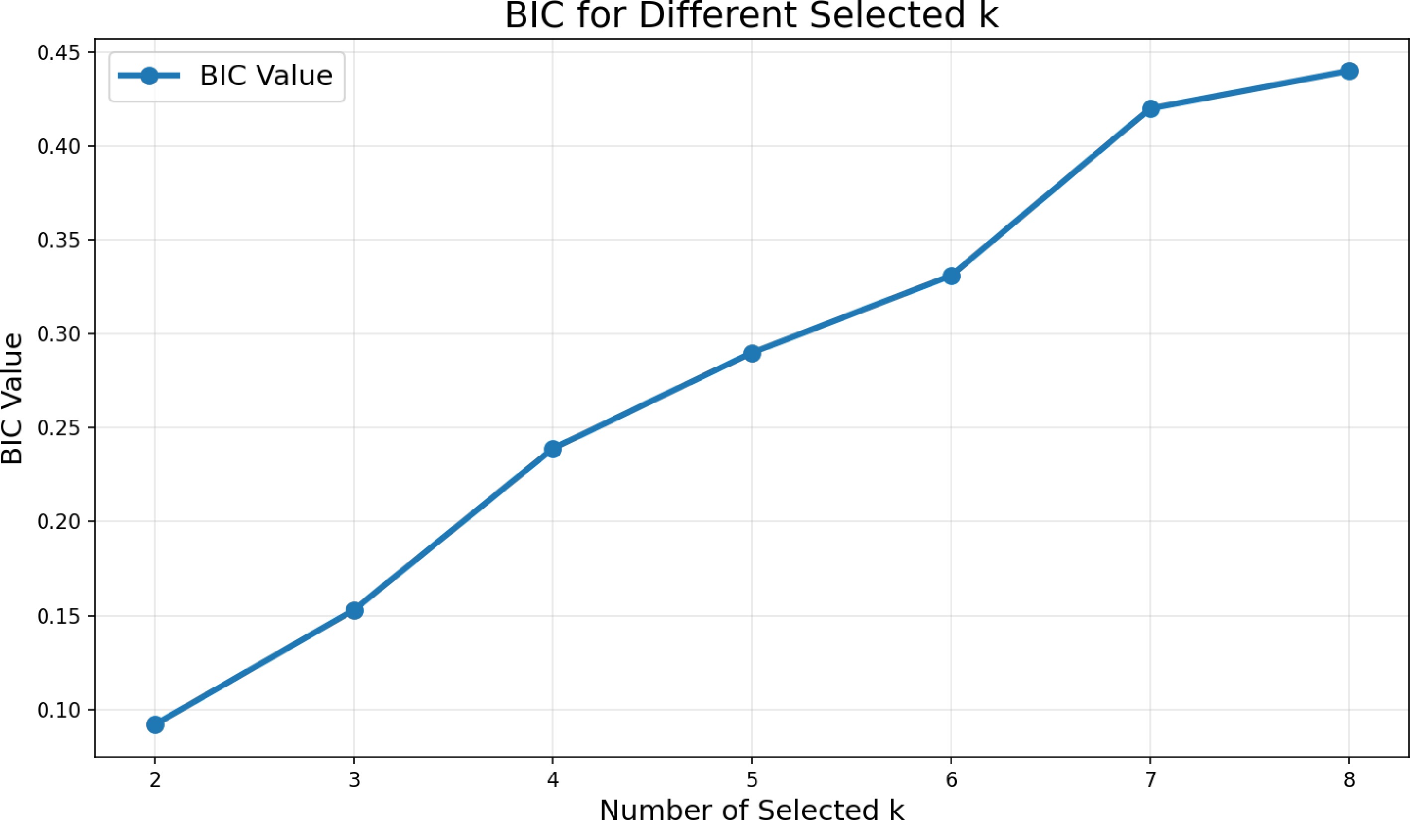
Figure 3.
BIC values for multiple selected k.
-
Input: Standardized training data $ \{( {\bf{x}}_i,y_i)\}_{i=1}^n $ $ \eta_0 $ $ N_{iter} $ Output: Trained weights $ {\bf{W}}_1 $ $ {\bf{b}}_1 $ $ {{\boldsymbol{\omega}}}_2 $ $ b_2 $ Initialize $ {\bf{W}}_1^{(1, 1)} $ $ {\bf{b}}^{(1, 1)}_1 $ $ {{\boldsymbol{\omega}}}^{(1, 1)}_2 $ $ b^{(1, 1)}_2 $ for $ t = 1 $ $ N_{iter} $ Shuffle the training data $ \{( {\bf{x}}_i,y_i)\}_{i=1}^n $ $ i = 1, 2, \cdots, n $ for $ i = 1 $ $ {{\boldsymbol{\omega}}}^{(t,i+1)}_2 \leftarrow {{\boldsymbol{\omega}}}^{(t,i)}_2 - \eta_t\dfrac{\partial \ell(y_i, f( {\bf{x}}_i;\cdots))}{\partial {{\boldsymbol{\omega}}}_2} $ $ b^{(t,i+1)}_2 \leftarrow b^{(t,i)}_2 - \eta_t\dfrac{\partial \ell(y_i, f( {\bf{x}}_i;\cdots))}{\partial b_2} $ $ {\bf{W}}^{(t,i+1)}_1 \leftarrow {\bf{W}}^{(t,i)}_1 - \eta_t\dfrac{\partial \ell(y_i, f( {\bf{x}}_i;\cdots))}{\partial {\bf{W}}_1} $ $ {\bf{b}}^{(t,i+1)}_1 \leftarrow {\bf{b}}^{(t,i)}_1 - \eta_t\dfrac{\partial \ell(y_i, f( {\bf{x}}_i;\cdots))}{\partial {\bf{b}}_1} $ end for Let $ {\bf{W}}^{(t)}_1 = {\bf{W}}^{(t,n+1)}_1 $ $ {\bf{w}}^{(t)}_{\cdot j} $ $ {\bf{W}}^{(t)}_1 $ Ranking $ \{\| {\bf{w}}^{(t)}_{\cdot j}\|_2\} $ $ \hat{S}^{(t)} $ $ \{\| {\bf{w}}^{(t)}_{\cdot j}\|_2\} $ Keep the $ {\bf{w}}^{(t)}_{\cdot j} $ $ j \in \hat{S}^{(t)} $ $ {\bf{w}}^{(t)}_{\cdot j} = \bf{0} $ $ j \notin \hat{S}^{(t)} $ Set $ {\bf{W}}^{(t+1, 1)}_1 = {\bf{W}}^{(t)}_1 $ $ {\bf{b}}^{(t+1, 1)}_1 = {\bf{b}}^{(t,n+1)}_1 $ $ {{\boldsymbol{\omega}}}^{(t+1,1)}_2 = {{\boldsymbol{\omega}}}^{(t,n+1)}_2 $ $ b^{(t+1, 1)}_2 = b^{(t,n+1)}_2 $ end for Table 1.
Multistage StoIHT algorithm.
-
Input: Standardized training data $ \{( {\bf{x}}_i,y_i)\}_{i=1}^n $ $ \eta_0 $ $ N_{iter} $ Output: Trained weights $ {\bf{W}}_1 $ $ {\bf{b}}_1 $ $ {{\boldsymbol{\omega}}}_2 $ $ b_2 $ Initialize $ {\bf{W}}_1^{(1, 1)} $ $ {\bf{b}}^{(1, 1)}_1 $ $ {{\boldsymbol{\omega}}}^{(1, 1)}_2 $ $ b^{(1, 1)}_2 $ for $ t = 1 $ $ N_{iter} $ Shuffle the training data $ \{( {\bf{x}}_i,y_i)\}_{i=1}^n $ $ i = 1, 2, \cdots, n $ for $ i = 1 $ $ {{\boldsymbol{\omega}}}^{(t,i+1)}_2 \leftarrow {{\boldsymbol{\omega}}}^{(t,i)}_2 - \eta_t\dfrac{\partial \ell(y_i, f( {\bf{x}}_i;\cdots))}{\partial {{\boldsymbol{\omega}}}_2} $ $ b^{(t,i+1)}_2 \leftarrow b^{(t,i)}_2 - \eta_t\dfrac{\partial \ell(y_i, f( {\bf{x}}_i;\cdots))}{\partial b_2} $ $ {\bf{W}}^{(t,i+1)}_1 \leftarrow {\bf{W}}^{(t,i)}_1 - \eta_t\dfrac{\partial \ell(y_i, f( {\bf{x}}_i;\cdots))}{\partial {\bf{W}}_1} $ $ {\bf{b}}^{(t,i+1)}_1 \leftarrow {\bf{b}}^{(t,i)}_1 - \eta_t\dfrac{\partial \ell(y_i, f( {\bf{x}}_i;\cdots))}{\partial {\bf{b}}_1} $ end for Let $ {\bf{W}}^{(t)}_1 = {\bf{W}}^{(t,n+1)}_1 $ $ {\bf{w}}^{(t)}_{\cdot j} $ $ {\bf{W}}^{(t)}_1 $ Ranking $ \left\{\| {\bf{w}}^{(t)}_{\cdot j}\|_2\right\} $ $ \hat{S}^{(t)} $ $ M_t $ $ \left\{\| {\bf{w}}^{(t)}_{\cdot j}\|_2\right\} $ Keep the $ {\bf{W}}^{(t)}_1 = [ {\bf{w}}^{(t)}_{\cdot j}] $ $ j \in \hat{S}^{(t)} $ $ {\bf{w}}^{(t)}_{\cdot j} $ $ j \notin \hat{S}^{(t)} $ Set $ {\bf{W}}^{(t+1, 1)}_1 = {\bf{W}}^{(t)}_1 $ $ {\bf{b}}^{(t+1, 1)}_1 = {\bf{b}}^{(t,n+1)}_1 $ $ {{\boldsymbol{\omega}}}^{(t+1,1)}_2 = {{\boldsymbol{\omega}}}^{(t,n+1)}_2 $ $ b^{(t+1, 1)}_2 = b^{(t,n+1)}_2 $ end for Table 2.
Multistage FSA algorithm.
-
Sample
sizeParameter Multistage FSA Multistage StoIHT IHT − HD-BIC BIC − HD-BIC BIC − HD-BIC BIC n = 1,000 Model size† 10 (0) 11.67 (1.556) 6 (0) 10 (0) 11.99 (1.972) 6 (0) 10 (0) 10.91 (1.167) 6 (0) FSR† 0.091 (0.071) 0.207 (0.113) 0 (0) 0.185 (0.074) 0.284 (0.135) 0 (0) 0.075 (0.099) 0.141 (0.120) 0 (0) NSR† 0.091 (0.071) 0.089 (0.073) 0.4 (0) 0.185 (0.074) 0.165 (0.077) 0.4 (0) 0.075 (0.099) 0.072 (0.094) 0.4 (0) RMSE† 1.745 (0.510) 1.743 (0.533) 3.333 (0.142) 2.353 (0.461) 2.234 (0.499) 3.222 (0.101) 1.520 (0.617) 1.492 (0.593) 3.197 (0.095) Time‡ 2.972 34.27 32.63 11.58 128.1 130.0 2.017 22.01 23.17 n = 1,500 Model size† 10 (0) 10.43 (0.711) 7.160 (1.815) 10 (0) 10.41 (0.861) 6.040 (0.398) 10 (0) 10.43 (0.778) 6 (0) FSR† 0.022 (0.044) 0.061 (0.075) 0.006 (0.024) 0.013 (0.034) 0.041 (0.068) 0 (0) 0.073 (0.094) 0.090 (0.106) 0 (0) NSR† 0.022 (0.044) 0.025 (0.048) 0.290 (0.173) 0.013 (0.034) 0.007 (0.026) 0.396 (0.040) 0.073 (0.094) 0.056 (0.089) 0.4 (0) RMSE† 1.192 (0.343) 1.228 (0.400) 2.802 (1.054) 1.119 (0.270) 1.075 (0.205) 3.206 (0.236) 1.467 (0.563) 1.368 (0.538) 3.179 (0.097) Time‡ 4.551 51.80 52.55 17.22 192.0 192.8 3.183 34.48 36.30 n = 3,000 Model size† 10 (0) 10.02 (0.140) 10 (0) 10 (0) 10.35 (0.921) 10 (0) 10 (0) 10.51 (0.877) 10.34 (0.681) FSR† 0 (0) 0.002 (0.013) 0 (0) 0 (0) 0.028 (0.067) 0 (0) 0.070 (0.094) 0.089 (0.100) 0.081 (0.098) NSR† 0 (0) 0 (0) 0 (0) 0 (0) 0 (0) 0 (0) 0.070 (0.094) 0.048 (0.083) 0.053 (0.085) RMSE† 1.192 (0.343) 1.228 (0.400) 2.802 (1.054) 1.119 (0.270) 1.075 (0.205) 3.206 (0.236) 1.467 (0.563) 1.313 (0.506) 1.347 (0.525) Time‡ 4.551 51.80 52.55 17.22 192.0 192.8 3.183 56.24 59.04 All experiments are conducted on 100 independent data sets. † Average FSR, NSR, and RMSE of test data are presented; ‡ average computational time (s). Table 1.
Comparison of the proposed multistage FSA, multistage StoIHT, and IHT methods for the high-dimensional linear regression model with the sample size n = 1,000, 1,500, and 3,000 and p0 = 2,000.
-
Sample
sizeParameter Multistage FSA Multistage StoIHT IHT − HD-BIC BIC − HD-BIC BIC − HD-BIC BIC n = 104 Model size† 6 (0) 8.270 (1.399) 5.850 (0.766) 6 (0) 7.810 (1.270) 6.120 (0.325) 6 (0) 7.640 (1.797) 5.120 (1.283) FSR† 0.100 (0.082) 0.309 (0.142) 0.070 (0.090) 0 (0) 0.212 (0.126) 0.017 (0.046) 0.275 (0,128) 0.401 (0.164) 0.172 (0.175) NSR† 0.100 (0.082) 0.077 (0.083) 0.102 (0.081) 0 (0) 0 (0) 0 (0) 0.275 (0,128) 0.278 (0.106) 0.323 (0.099) RMSE† 2.518 (0.176) 2.453 (0.168) 2.543 (0.222) 1.506 (0.084) 1.531 (0.082) 1.519 (0.082) 2.888 (0.207) 2.943 (0.183) 3.020 (0.198) Time‡ 23.78 195.6 192.8 27.75 223.5 219.7 10.80 83.04 89.33 n = 2 × 10⁴ Model size† 6 (0) 8.150 (1.352) 6.350 (0.684) 6 (0) 8.180 (1.403) 6.090 (0.286) 6 (0) 7.740 (1.659) 6.510 (1.895) FSR† 0.015 (0.048) 0.257 (0.125) 0.059 (0.094) 0 (0) 0.243 (0.139) 0.013 (0.041) 0.282 (0.122) 0.406 (0.164) 0.291 (0.205) NSR† 0.015 (0.048) 0.017 (0.050) 0.013 (0.045) 0 (0) 0 (0) 0 (0) 0.282 (0.122) 0.267 (0.139) 0.283 (0.130) RMSE† 2.110 (0.150) 2.087 (0.159) 2.076 (0.159) 1.408 (0.075) 1.393 (0.083) 1.390 (0.083) 2.906 (0.210) 2.885 (0.280) 2.943 (0.308) Time‡ 47.67 379.9 386.5 55.51 457.8 446.5 18.11 156.6 162.2 n = 3 × 10⁴ Model size† 6 (0) 7.790 (1.409) 6.610 (0.937) 6 (0) 7.760 (1.556) 6.020 (0.140) 6 (0) 7.660 (1.589) 6.590 (1.650) FSR† 0.007 (0.033) 0.209 (0.148) 0.080 (0.113) 0 (0) 0.195 (0.159) 0.003 (0.020) 0.252 (0.124) 0.388 (0.159) 0.296 (0.180) NSR† 0.007 (0.033) 0.007 (0.033) 0.003 (0.023) 0 (0) 0 (0) 0 (0) 0.252 (0.124) 0.252 (0.119) 0.267 (0.120) RMSE† 1.823 (0.149) 1.816 (0.143) 1.800 (0.130) 1.357 (0.080) 1.358 (0.069) 1.354 (0.067) 2.859 (0.242) 2.852 (0.246) 2.876 (0.241) Time‡ 72.70 587.9 586.0 82.18 682.6 670.2 33.98 264.8 268.5 All experiments are conducted on 100 independent data sets. †Average FSR, NSR, and RMSE of the test data are presented; ‡average computational time (s). Table 2.
Comparison of the multistage FSA, multistage StoIHT, and IHT methods for the nonlinear regression model with the sample size n = 104, 2 × 10⁴, 3 × 10⁴ , and p0 = 1,000.
-
Sample
sizeParameter Multistage FSA Multistage StoIHT IHT − HD-BIC BIC − HD-BIC BIC − HD-BIC BIC n = 104 Model size† 6 (0) 6.530 (0.830) 4.680 (0.760) 6 (0) 5.450 (1.982) 4.020 (0.140) 6 (0) 7.500 (1.825) 4.040 (0.196) FSR† 0.072 (0.118) 0.135 (0.161) 0.021 (0.069) 0.650 (0.065) 0.580 (0.131) 0.497 (0.088) 0.330 (0.023) 0.411 (0.146) 0.248 (0.010) NSR† 0.072 (0.118) 0.073 (0.134) 0.238 (0.125) 0.650 (0.065) 0.652 (0.075) 0.663 (0.058) 0.330 (0.023) 0.305 (0.071) 0.493 (0.033) AUC† 0.960 (0.008) 0.959 (0.011) 0.942 (0.021) 0.903 (0.015) 0.903 (0.016) 0.902 (0.015) 0.933 (0.009) 0.936 (0.013) 0.904 (0.013) Time‡ 24.22 201.6 196.3 44.29 365.7 375.2 12.23 105.1 101.6 n = 2 × 10⁴ Model size† 6 (0) 7.460 (1.315) 5.890 (0.467) 6 (0) 6.880 (1.856) 4.310 (0.523) 6 (0) 7.670 (1.750) 5.190 (0.674) FSR† 0.013 (0.056) 0.175 (0.138) 0.005 (0.027) 0.512 (0.114) 0.505 (0.159) 0.317 (0.157) 0.330 (0.023) 0.426 (0.133) 0.219 (0.065) NSR† 0.013 (0.056) 0.003 (0.023) 0.023 (0.078) 0.512 (0.114) 0.468 (0.112) 0.515 (0.100) 0.330 (0.023) 0.302 (0.073) 0.332 (0.029) AUC† 0.967 (0.007) 0.967 (0.006) 0.956 (0.049) 0.915 (0.016) 0.918 (0.018) 0.915 (0.017) 0.934 (0.009) 0.938 (0.013) 0.934 (0.009) Time‡ 50.43 398.4 397.6 88.29 711.3 750.4 22.64 198.6 189.5 n = 3 × 10⁴ Model size† 6 (0) 8.810 (1.102) 5.970 (0.386) 6 (0) 4.710 (1.458) 4.050 (0.218) 6 (0) 7.640 (1.616) 5.450 (1.117) FSR† 0.008 (0.036) 0.309 (0.100) 0.008 (0.033) 0.350 (0.055) 0.150 (0.173) 0.075 (0.112) 0.332 (0.017) 0.431 (0.119) 0.244 (0.097) NSR† 0.008 (0.036) 0.003 (0.023) 0.013 (0.061) 0.350 (0.055) 0.367 (0.067) 0.377 (0.073) 0.332 (0.017) 0.303 (0.080) 0.330 (0.053) AUC† 0.967 (0.007) 0.968 (0.006) 0.962 (0.034) 0.936 (0.008) 0.935 (0.008) 0.934 (0.009) 0.933 (0.008) 0.938 (0.014) 0.935 (0.012) Time‡ 73.86 592.2 592.6 124.3 1069 1138 33.84 256.8 250.2 All experiments are conducted on 100 independent data sets. † Average FSR, NSR, and AUC for test data are presented; ‡ average computational time (s). Table 3.
Comparison of the multistage FSA, multistage StoIHT, and IHT methods for the nonlinear logistic regression model with the sample size n = 104, 2 × 10⁴, 3 × 10⁴, and p0 = 1,000.
-
Parameter Multistage FSA Multistage StoIHT IHT − HD-BIC BIC − HD-BIC BIC − HD-BIC BIC k* = 3 Model size† 3 (0) 3.580 (0.982) 1 (0) 3 (0) 6.940 (0.276) 1 (0) 3 (0) 1.160 (0.913) 1 (0) FSR† 0.277 (0.430) 0.333 (0.405) 0.250 (0.433) 0.870 (0.199) 0.834 (0.117) 0.880 (0.325) 0.997 (0.033) 0.887 (0.313) 0.890 (0.313) NSR† 0.277 (0.430) 0.253 (0.419) 0.750 (0.144) 0.870 (0.199) 0.613 (0.274) 0.960 (0.108) 0.997 (0.033) 0.957 (0.112) 0.963 (0.104) AUC† 0.848 (0.227) 0.856 (0.225) 0.501 (0.020) 0.505 (0.053) 0.522 (0.110) 0.500 (0.019) 0.500 (0.009) 0.500 (0.000) 0.500 (0.000) Time‡ 2.378 18.58 19.81 2.833 22.64 23.22 4.458 17.71 17.59 k* = 4 Model size† 4 (0) 6.130 (1.101) 1 (0) 4 (0) 7 (0) 1 (0) 4 (0) 1 (0) 1 (0) FSR† 0.290 (0.396) 0.473 (0.260) 0.320 (0.466) 0.840 (0.175) 0.786 (0.132) 0.880 (0.325) 1 (0) 0.850 (0.357) 0.850 (0.357) NSR† 0.290 (0.396) 0.223 (0.337) 0.830 (0.117) 0.840 (0.175) 0.625 (0.230) 0.970 (0.081) 1 (0) 0.963 (0.089) 0.963 (0.089) AUC† 0.812 (0.231) 0.823 (0.221) 0.497 (0.018) 0.498 (0.019) 0.506 (0.050) 0.497 (0.020) 0.498 (0.010) 0.500 (0.001) 0.500 (0.001) Time‡ 2.615 20.51 20.47 2.788 24.52 24.50 4.611 17.46 17.43 k* = 5 Model size† 5 (0) 6.590 (0.750) 1 (0) 5 (0) 7 (0) 1 (0) 5 (0) 1 (0) 1 (0) FSR† 0.636 (0.313) 0.624 (0.264) 0.610 (0.488) 0.792 (0.160) 0.734 (0.146) 0.830 (0.376) 0.998 (0.020) 0.820 (0.384) 0.820 (0.384) NSR† 0.636 (0.313) 0.512 (0.325) 0.922 (0.098) 0.792 (0.160) 0.628 (0.204) 0.966 (0.075) 0.998 (0.020) 0.964 (0.077) 0.964 (0.077) AUC† 0.573 (0.166) 0.598 (0.185) 0.500 (0.019) 0.503 (0.020) 0.508 (0.048) 0.500 (0.017) 0.498 (0.011) 0.500 (0.000) 0.500 (0.000) Time‡ 2.616 20.88 20.97 2.828 25.30 23.83 4.618 17.37 17.57 All experiments are conducted on 100 independent data sets. † Average FSR, NSR, and AUC for test data are presented; ‡ average computational time (s). Table 4.
Comparison of the multistage FSA, multistage StoIHT, and IHT methods for the XOR model with sample size n = 3,000 and p0 = 20.
-
Number of selected variables Multistage FSA Multistage StoIHT IHT k = 2 0.991 (0.064) 0.991 (0.064) 0.991 (0.065) k = 3 0.988 (0.065) 0.992 (0.062) 0.993 (0.056) k = 4 0.987 (0.065) 0.994 (0.062) 0.989 (0.059) The RMSE values for validation data are presented. Table 5.
Comparison of the multistage FSA, multistage StoIHT, and IHT methods for 17-AAG data set.
-
Multistage FSA Multistage StoIHT IHT Lasso k* Known 0.642 (0.021) 0.535 (0.029) 0.534 (0.040) 0.608 (0.013) BIC 0.656 (0.022) 0.533 (0.062) 0.522 (0.040) 0.610 (0.011) HD-BIC 0.651 (0.029) 0.532 (0.049) 0.519 (0.039) − The average AUC values for validation data are presented. Table 6.
Comparison of the multistage FSA, multistage StoIHT, and IHT methods for the Madelon data set.
Figures
(3)
Tables
(8)