Feature selection with annealing for shallow neural networks using the multistage stochastic algorithm

Feature selection is a fundamental topic of research in statistics and machine learning, as it improves predictive accuracy, enhances interpretability, and reduces computational costs by eliminating irrelevant or redundant variables. Consequently, it has been widely used in real-world data analysis across various application domains.

Several methods for variable selection have been proposed for both parametric and nonparametric models. The classical techniques include the $ \ell_0 $-penalized approach^[1,2], the $ \ell_1 $-penalized method^[3−5], as well as the SCAD^[6] and MCP^[7] methods. In addition, group-penalized methods, such as group Lasso^[8] and adaptive group Lasso^[9], have been proposed for variable selection. Although these methods are widely applied in practice, they have primarily been developed for high-dimensional linear and generalized linear models. Extensions to high-dimensional varying-coefficient models^[10] and sparse additive models^[11] have also been explored, which are, however, less applicable to neural networks.

Being a fundamental component of deep learning, neural networks have undergone significant theoretical and empirical advances, and can now be used to approximate complex data structures and tackle intricate modeling tasks^[12−16]. However, neural networks are often over-parameterized, posing challenges for training, prediction, and interpretation. Several methods have been developed to reduce the number of model parameters and compress network architectures in order to enhance the predictive performance. A widely adopted solution is dropout^[17], which randomly drops nodes during training to prevent overfitting. Subsequently, sparse neural networks have been proposed to reduce the number of parameters and compress model architectures. The existing research on sparse neural networks falls into two categories: Bayesian and frequentist. Within the Bayesian framework, various sparsity-inducing priors, such as the hierarchical prior^[18,19], the mixture Gaussian prior^[20], and the spike-and-slab prior^[21], have been proposed for learning sparse Bayesian neural networks. In the frequentist framework, the group $ \ell_1 $-regularized methods^[22−25] have been proposed to learn sparse neural networks. In addition, node pruning techniques^[26,27] have been introduced to compress neural network architectures.

Although the existing methods encourage sparsity in the weight matrix and compress the network architectures, few methods directly address the sparse-input problem. However, these methods are not specifically designed for variable selection. To identify the important covariates in neural network models, several nonlinear variable selection techniques have been proposed. First, the group $ \ell_1 $ penalty is applied to induce sparsity into the input weight matrix^[28]. Next, an additional selection layer is introduced, and both $ \ell_0 $^[29] and $ \ell_1 $^[30] penalties are used for variable selection. More recently, a group $ \ell_0 $-regularized method has been proposed for variable selection^[31], using the iterative hard-thresholding (IHT) algorithm to estimate the parameters^[32]. Furthermore, the concept of group $ \ell_0 $ penalty has been extended to nonparametric expectile regression within the framework of deep neural networks^[33].

However, the current neural network-based variable selection methods face challenges in both variable selection accuracy and predictive performance. First, these $ \ell_1 $-penalized neural network approaches rely heavily on tuning parameters, leading to instability in both variable selection and prediction. Moreover, using the $ \ell_1 $ penalty may incur unwanted bias and lead to inconsistency in variable selection^[5,34]. Therefore, the $ \ell_0 $ penalty may be an ideal choice, as it does not incur any bias^[2].

Just like the $ \ell_1 $ penalty is associated with the soft-thresholding operator, the $ \ell_0 $ penalty corresponds to the hard-thresholding operator^[35]. Accordingly, the IHT algorithm^[32], which combines gradient descent with a hard-thresholding operator, has been proposed to minimize $ \ell_0 $-penalized loss functions. Although this gradient-based approach is computationally efficient and easy to implement, it may converge to the local optima when applied to neural networks. Moreover, $ \ell_0 $- and $ \ell_1 $-regularized methods require users to prespecify the number of selected variables k and the regularization parameter λ.

In comparison with the IHT algorithm, which is based on deterministic learning^[31], we propose the multistage stochastic iterative hard-thresholding (StoIHT) algorithm. The proposed methods, which are based on stochastic learning algorithms, are used to select important variables by estimating the weights connecting the input and the first hidden layer. Then, we develop a novel variable selection method with an annealing strategy within the framework of a multistage stochastic algorithm^[36]. This approach can help in substantially enhancing both variable selection and prediction accuracy. To simplify the discussion and provide a clear description of our methodology, we will focus on shallow neural networks in this article. Furthermore, we investigate the criteria for variable selection and develop a novel Bayesian information criterion (BIC) tailored to the high-dimensional setting (the large-p−small-n scenario), along with the conventional BIC for the low-dimensional setting (n > p scenario)^[37]. The main contributions of this paper are as follows:

(1) This article proposes two novel variable selection methods that use neural networks as surrogate models with a group $ \ell_0 $ penalty. To enhance the selection accuracy, we introduce an annealing strategy and develop a multistage stochastic optimization framework to identify key variables. The performance and effectiveness of the proposed methods are demonstrated through numerical experiments and real-data applications.

(2) This paper develops a novel BIC for model selection in the high-dimensional setting. Numerical experiments demonstrate that the proposed criterion helps to substantially improve variable selection accuracy relative to the conventional BIC.

The remainder of this paper is organized as follows. The next section introduces the notation and outlines the model framework. The section "Methodology" presents the proposed variable selection approaches based on a stochastic optimization strategy. The section "Simulation" assesses the performance of the proposed methods through numerical experiments and real data applications. The last section provides the conclusions and discusses the potential directions for future research.

Given a collection of independent training instances $ \{({\bf{x}}_i, y_i)\}_{i=1}^n $, where $ {\bf{x}}_i \in \mathbb{R}^{p_0} $ represents a sample of input features and $ y_i \in \mathbb{R} $ denotes the corresponding output, we consider the following nonparametric regression model:

where, $ f^* $ represents the unknown true model relating the input $ {\bf{x}}_i $ to the output $ y_i $, and $ \epsilon_i $ is the random noise term assumed to have a Gaussian distribution with mean zero and variance σ². Suppose that p₀ is large and $ f^* $ in Eq. (1) only depends on a subset of the input features, which are referred to as important features. In other words, there exists an unknown index set $ S^* \subset \{1, 2, \ldots, p_0\} $ with $ |S^*| = k^* \ll p_0 $, where $ k^* $ denotes the number of important features. Moreover, we can extend the previous setting to the nonparametric logistic regression model:

where, $ f^* $ represents the unknown relationship between the input $ {\bf{x}}_i $ and the log-odds of the binary outcome $ y_i \in \{0,1\} $. In the literature of neural networks^[14,15,31], $ f^* $ is often assumed to belong to the $ (d, C) $-smoothness function class, which is presented in Definition 2.1.

Definition 2.1. Let d = q + ζ, where $ \zeta \in $(0, 1] and q = $ \left\lfloor d \right\rfloor \in \mathbb{N}_0 $ denotes the largest integer strictly smaller than d ($ \mathbb{N}_0 $ denotes the set of nonnegative integers). A function $ f:\mathbb{R}^{p_0} \rightarrow \mathbb{R} $ is called $ (d, C) $-smooth function if for every $ {{\boldsymbol{\alpha}}} = (\alpha_1, \alpha_2, \cdots, \alpha_{p_0})^{\top} \in \mathbb{N}^{p_0}_0 $ with $ \sum_{j=1}^{p_0}\alpha_j = q $, the partial derivative $ \partial^{q}f/\partial x_{1}^{\alpha_1}\partial x_{2}^{\alpha_2} \cdots \partial x_{p_0}^{\alpha_{p_0}} $ exists and satisfies

for all $ {\bf{x}}_1, {\bf{x}}_2 \in \mathbb{R}^{p_0} $, where $ \|\cdot\|_2 $ denotes the $ \ell_2 $-norm, otherwise known as the Euclidean norm.

In this paper, we aim to estimate the index set $ S^* $ from the given training data and to simultaneously approximate the underlying function $ f^* $. To address the feature selection and model learning problems, we employ a one-hidden-layer neural network as a surrogate to approximate the unknown true function $ f^* $. We now introduce the class of one-hidden-layer neural networks used throughout this paper. Let $ {\cal{H}}_{p_1, \varphi} $ denote the class of one-hidden-layer neural networks with width $ p_1 $ and activation function φ:

Therefore, models (1) and (2) can be approximated as

and

respectively, where $ {\bf{W}}_1 \in \mathbb{R}^{p_1 \times p_0} $ is the weight matrix connecting the input layer to the first hidden layer, and $ {\bf{b}}_1 \in \mathbb{R}^{p_1} $ is the bias vector. The vector $ {{\boldsymbol{\omega}}}_2 \in \mathbb{R}^{p_1} $ represents the weights from the hidden layer to the output layer, with a bias term $ b_2 \in \mathbb{R} $. The activation function $ \varphi:\mathbb{R}^{p_1} \rightarrow \mathbb{R}^{p_1} $ is coordinate-wise and piecewise differentiable function. We use the $ ReLU $ function $ \varphi(x) = \max\{x,0\} $ in this article. Let $ \ell(y_i, f( {\bf{x}}_i)) $ be the loss function for each training instance $ ( {\bf{x}}_i, y_i) $, where $ f( {\bf{x}}_i) = {{\boldsymbol{\omega}}}^{\top}_2\varphi( {\bf{W}}_1 {\bf{x}}_i+ {\bf{b}}_1) + b_2 $ represents the one-hidden-layer neural network model. Hence, the empirical loss function based on n samples is

We propose the following optimization problem with a sparsity constraint on the weight matrix to address the feature selection problem:

where, $ \| {\bf{W}}_1\|_{2,0} = \#\{j:\| {\bf{w}}_{\cdot j}\|_2 \neq 0, j = 1, 2, \cdots, p_0\} $ and $ {\bf{w}}_{\cdot j} $ denotes the j-th column of the weight matrix $ {\bf{W}}_1 $. Therefore, $ \| {\bf{W}}_1\|_{2,0} $ corresponds to the number of nonzero column vectors of $ {\bf{W}}_1 $. The index set of the nonzero columns of $ {\bf{W}}_1 $ is denoted by S.

It is worth noting that the group $ \ell_0 $ penalty is similar to conventional group penalty methods^[8]: if predictor j is unimportant, all entries in the vector $ {\bf{w}}_{\cdot j} $ are zero; otherwise, all entries in the vector $ {\bf{w}}_{\cdot j} $ are nonzero. Figure 1 shows the architecture of the one-hidden-layer neural network model derived using the group $ \ell_0 $ penalty. This architecture can be naturally extended to deep neural networks, as the sparsity constraint is independent of the hidden layers. Since neural networks are interpreted as surrogate models approximating the unknown model $ f^{*} $, assuming that $ f^{*} $ belongs to the $ (d, C) $-smooth function class, we can pre-select the neural network architecture to achieve a desired approximation error. We then formulate the feature selection problem as shown by Eq. (3). In other words, $ p_{1} $, which denotes the number of neurons in the first hidden layer, is fixed by solving the feature selection problem in Eq. (3).

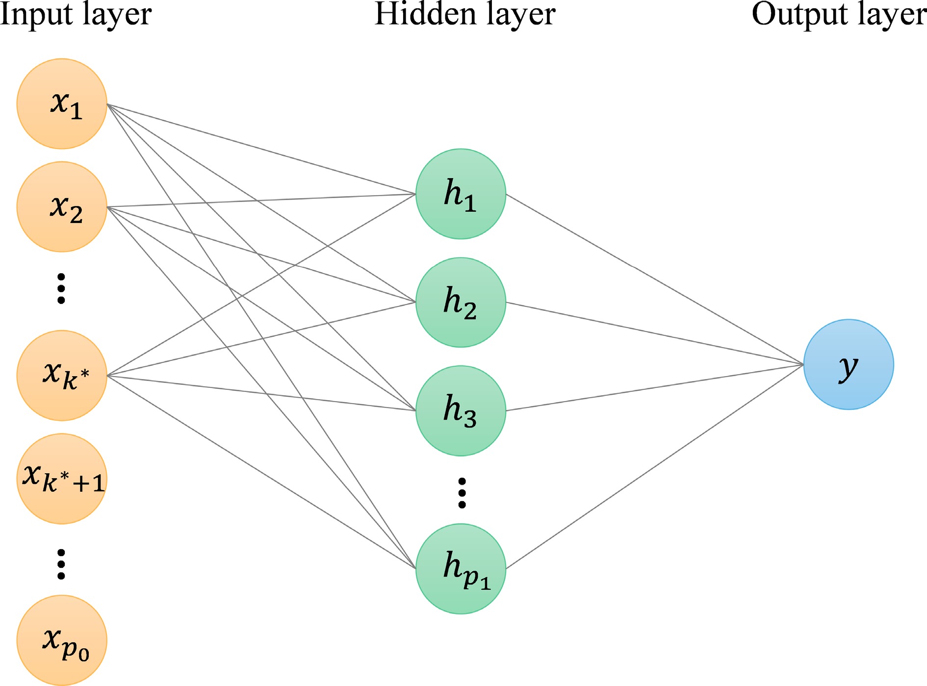
Figure 1. 

The architecture of a one-hidden-layer neural network derived using the group $ \ell_0 $ penalty is illustrated. For simplicity, the bias terms are omitted. The figure shows that there are no edges between the input nodes $ {x_{k^*+1}, \cdots , x_{p_0}} $ and the neurons in the hidden layer, indicating that the $ (k^*+1) $-th to $ p_0 $-th column vectors of $ {\bf{W}}_1 $ are zeros. This sparsity pattern is induced by the group $ \ell_0 $ penalty.

We now delineate the notations used throughout the paper. Vectors are denoted by lowercase bold letters, such as $ {\bf{x}} \in \mathbb{R}^d $, and scalars by lowercase letters, for example, $ x \in \mathbb{R} $. Subscripts index a sequence of vectors, for example $ {\bf{w}}_1, {\bf{w}}_2, \ ... $. The components of a vector are indicated by nonbold subscripts, such as $ w_j $. Matrices are represented by uppercase bold letters, for example, $ {\bf{M}} \in \mathbb{R}^{d \times d} $, while random variables are denoted by uppercase letters, such as Z. For a vector $ {{\boldsymbol{\gamma}}} = (\gamma_1, \gamma_2, \cdots, \gamma_n)^{\top} \in \mathbb{R}^n $, we use the following norms: $ \| {{\boldsymbol{\gamma}}}\|_1 = \sum_{i=1}^{n} |\gamma_i| $, $ \| {{\boldsymbol{\gamma}}}\|_2 = \sqrt{\sum_{i=1}^{n} \gamma_i^2} $, and $ \| {{\boldsymbol{\gamma}}}\|_0 = \#\{i : \gamma_i \neq 0\} $.

In the section "Setting and notation," we introduce the feature selection problem and derive the corresponding constrained optimization problem (Eq. [3]) using a one-hidden-layer neural network as a surrogate model. In this section, we propose two variable selection methods within a multistage stochastic learning framework to solve the constrained optimization problem (Eq. [3]). To mitigate the risk of gradient descent converging to local optima, we first extend the IHT algorithm^[31,32] to a multistage StoIHT algorithm^[38] to train a one-hidden-layer neural network. Next, we develop a variant of StoIHT that uses an annealing strategy for variable selection, known as feature selection with annealing (FSA). Compared with the existing IHT method, the proposed multistage StoIHT and multistage FSA methods show a superior overall performance on regression and classification tasks, as validated by numerical experiments.

Multistage stochastic IHT

We begin by introducing the multistage stochastic learning framework. In the stochastic algorithm, each iteration operates on only a mini-batch of the data set, dividing the training process into distinct stages, each comprising several iterations. This staged training structure enables the use of different learning rates and other hyperparameters across stages. The output of the current training stage is used as the initial value for the subsequent stage. In neural network training, a stage can naturally correspond to a single epoch.

Then, we introduce the StoIHT algorithm within a multistage framework. The algorithm consists of N_iter stages. In each stage, the stochastic gradient descent (SGD) algorithm updates model parameters using only a mini-batch of data per iteration, thereby introducing randomness into the parameter updates. Consequently, applying a hard-thresholding operator immediately after each iteration may yield poor variable selection performance^[39]. To address this issue, we apply the hard-thresholding operator after all the SGD iterations within a stage are complete, thereby stabilizing the variable selection procedure. Recall that the hard-thresholding operator selects the top-k column vectors of the weight matrix $ {\bf{W}}_1 $ based on the $ \ell_2 $-norms and sets the rest of the column vectors to zeros. At the end of each stage, the resulting weight matrix, after implementing a hard-thresholding operator, is consistent with the constraint in the optimization problem (3). All parameter estimates from the shallow neural network model at each stage are treated as the initial values for the next stage. In other words, the multistage StoIHT algorithm stabilizes the variable selection procedure by using the hard-thresholding output of the current stage as a "warm start" for stochastic learning in the next stage. The multistage StoIHT algorithm is summarized in Algorithm 1. When N_iter = 1, the multistage StoIHT algorithm is equivalent to the SGD with truncation algorithm^[39].

Multistage FSA

In this section, we present the proposed multistage FSA method. As the true variables may not reveal their significance early in an iterative algorithm, the $ \ell_2 $-norm of their updated parameters $ \| {\bf{w}}_{\cdot j}\|_2 $ may not rank among the top-k largest values. As a result, these true variables could be excluded by setting their weights to zero, preventing their selection.

To address the abovementioned challenge and enhance the selection accuracy, we propose a variable selection method that incorporates an annealing strategy. After all iterations in a given stage are completed, we retain only those variables whose $ \ell_2 $-norm of updated parameter vectors $ \|{\bf{w}}^{(t)}_{\cdot j}\|_2 $ ranks among the top-$ M_t $ largest values. Variables with smaller $ \|{\bf{w}}^{(t)}_{\cdot j}\|_2 $ values are considered unimportant and will be removed. Their parameters will not be updated in subsequent iterations. An annealing schedule for $ M_t $ has been proposed^[1,39], representing the number of features kept at the t-th iteration such that

where, $ p_0 $ is the total number of variables, k is the desired sparsity level, μ is the annealing parameter, and $ N_{iter} $ is the total number of iterations for this schedule when exactly k features are selected.

Figure 2 illustrates the annealing schedule for various annealing parameters $\mu $. A larger $\mu $ leads to a sharp decline in the number of retained variables $ M_t $ in the initial stage, whereas a smaller $\mu $ results in a far more gradual decrease. Compared with linear decay, the annealing schedule is computationally more efficient, as it truncates more input variables and reduces the dimensionality of the neural network weight parameters in the first few iterations. The multistage FSA algorithm is summarized in Algorithm 2.

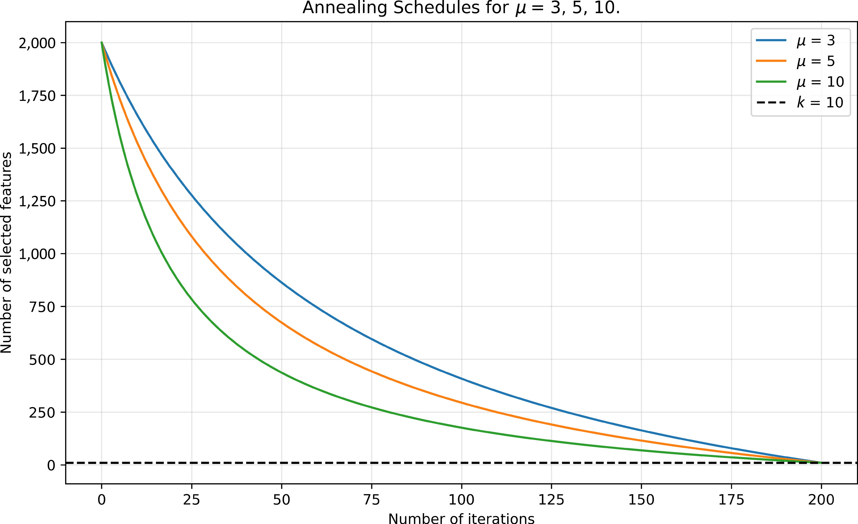
Figure 2. 

Annealing schedule for p₀ = 2,000, k = 10, N_iter = 200, and multiple annealing parameters $ \mu $ = 3, 5, and 10.

Given that the neural network models are trained with SGD per epoch, backpropagation is performed accordingly. As a result, $ {{\boldsymbol{\omega}}}_2 $ and $ b_2 $ are updated first, followed by the updates of $ {\bf{W}}_1 $ and $ {\bf{b}}_1 $. While sharing the same SGD iterations in each stage, Algorithm 1 employs a hard-thresholding operator and sets the unimportant weights to zero, keeping only k variables. Algorithm 2 removes the unimportant variables according to the current schedule $ M_{t} $, which reaches k in the last stage. It is worth noting that during the annealing procedure, the learning rate may need to be adapted based on the number of remaining variables $ M_t $, due to changes in the problem dimensions^[2]. Consequently, the learning rate is kept constant within each stage but decays across stages.

The BIC for neural network models

Since the true number of features $ k^* $ is generally unknown in practice, it is necessary to determine the number of relevant features using a model selection criterion. In the neural network model, we can select the number of variables k using the BIC^[37]. According to the conventional definition of the BIC for a sparse model^[40], the BIC value for a one-hidden-layer neural network model is given by

where, p₁ denotes the width of the hidden layer, k is the selected number of variables, and n is the sample size. Eq. (4) is based on the fact that the number of free parameters in a one-hidden-layer neural network satisfying the sparsity constraint in Eq. (3) is of order $ O(k \cdot p_1) $.

However, in the high-dimensional scenario with sample size n < p₀, an increase in the number of parameters k causes the penalty term $ k \cdot p_1 \cdot \log(n)/n $ to intensify sharply. Consequently, to avoid excessive penalization, the variable selection criterion inevitably favors models with smaller k, which increases the risk of omitting important variables. To address this issue, a novel high-dimensional BIC (HD-BIC) is proposed:

Here, we modify the penalty term in Eq. (4) to $ k \cdot \log(p_1) \cdot \log(n)/n $ for enabling the model to select a more inclusive set of important variables. Furthermore, the high-dimensional setting corresponds to the few-shot supervised learning paradigm within the proposed feature selection framework, particularly when neural networks are employed as the surrogate model. The modification introduced to the penalty term enables us to incorporate neural networks with wider hidden layers, thereby introducing a moderate degree of over-parameterization. Such a design effectively alleviates the difficulties posed by insufficient training samples, a critical challenge commonly encountered in high-dimensional few-shot scenarios. The numerical results for these two BIC values are reported in the experiments of the section "Simulation".

A comparison of existing feature selection methods in neural networks

The methods introduced in this paper, regardless of the specific algorithmic details, can be broadly classified as nonparametric feature selection techniques. In these approaches, surrogate models are employed to approximate the underlying model. The index set $ S^{*} $ is estimated by determining the parameters of the surrogate models from the available data. Given the powerful approximation capabilities of neural networks, many studies have leveraged them as surrogate models. In this section, we review the relevant studies to the best of the our knowledge and compare their methodologies with those in our own work.

In the literature of the latest method^[41], the authors estimate the index set of the nonzero columns of $ {\bf{W}}_1 $ using a second-order Stein's formula and establish consistency results under the sub-Gaussian assumption on the input covariates and Hölder continuity of the underlying model. Although the resulting estimator is independent of the neural network architecture, the proposed algorithms rely on accurate estimation of the inverse covariance matrix, which is challenging in high dimensions. As variants of the SGD algorithm, our methods incur low storage costs in the high-dimensional setting and are independent of the distribution of the input variables.

In works featuring Deep Feature Selection^[29] and LassoNet^[30], the sparsity constraint is imposed on $ {\bf{W}}_1 $, leading to a sparse-constrained nonconvex optimization problem that is typically solved using Alternating Direction Method of Multipliers (ADMM) algorithms. Although our methods address the same class of constrained optimization problems, we instead adopt the “Slow Kill” strategy^[2], which gradually enforces sparsity through a multistage feature selection procedure. Moreover, the optimization at each stage is not restricted to SGD; the corresponding iterations can be implemented using any mainstream machine-learning optimization algorithm, thereby providing greater flexibility and additional modeling capabilities.

In this section, we describe the evaluation of the proposed variable selection methods using a one-hidden-layer neural network. First, we present the simulation results for a high-dimensional linear regression model as an initial example. Next, we evaluate the performance of the proposed variable selection methods on the nonlinear regression model using large-scale data sets. We then extend the nonlinear regression model to the nonlinear logistic regression model. In addition, we tackle a particularly challenging Exclusive OR (XOR) problem^[42]. Finally, we present the results of the real-data analysis. Each simulation setting is repeated 100 times using independently generated data sets, and the cosine-annealing method is used to schedule the learning-rate decay. Since initializing neural network parameters to zero leads to symmetry issues during training, we adopt randomized initialization schemes proposed in the literature^[43]. The number of hidden-layer nodes is set to 128 for all experiments, except for the XOR problem, where it is increased to 256. All simulations are performed on a desktop equipped with an AMD Ryzen 9 9950X3D CPU running at 4.30 GHz and 64 GB of memory.

High-dimensional linear regression case

Here, we present the results of a numerical experiment for a high-dimensional linear regression model. The samples $ {\bf{x}}_i \in \mathbb{R}^{p_0} $, for $ i = 1, 2, \cdots, n $, are generated from a multivariate Gaussian distribution with mean zero and an AR(2) covariance matrix $ {{\boldsymbol{\Sigma}}} $, which has the structure:

The response $ y_i $ is generated using the high-dimensional linear regression model

where, the parameter vector β^* = (2, −2, 2, 3, 3, −2, 3, 3, −3, 2, 0, 0, ..., 0)^T$ \in \mathbb{R}^{p_0} $, and $ \epsilon_i $ is the random noise term. In this simulation, we set p₀ = 2,000 and sample sizes n = 1,000, 1,500, and 3,000. We also generate test data with sample size n = 1,000.

In this simulation, we compare the performance of the proposed multistage StoIHT method with the multistage FSA method. We also include the IHT method as a baseline^[31]. First, we consider the case in which the number of variables $ k^* $ is known. Next, we assume that the number of variables $ k^* $ is unknown and use both the conventional BIC and the proposed HD-BIC, as defined in Eqs. (4) and (5), for variable selection. The evaluation criteria for prediction performance and variable selection include model size (i.e., the number of selected covariates), false selection rate (FSR), negative selection rate (NSR)^[44,45], and root-mean-square error (RMSE) for the test data. The FSR and NSR are defined as

where, $ S^* $ denotes the index set of true important covariates and $ \hat{S} $ is the estimated index set. The results for the numerical experiments are presented in Table 1.

From Table 1, we observe that the performances of the multistage StoIHT and multistage FSA methods are similar in this high-dimensional linear regression setting. Specifically, in the high-dimensional scenario with n = 1,000 and p₀ = 2,000, the multistage FSA outperforms the multistage StoIHT and the IHT when using the proposed HD-BIC. As the sample size n increases, the multistage StoIHT performs slightly better than the multistage FSA. When the sample size n is sufficiently large, for example, n = 3,000, the results obtained with the conventional BIC are better than those obtained with the HD-BIC. We also conclude that multistage FSA and multistage StoIHT outperform the IHT method in the large-n case.

Nonlinear regression case

The numerical results for the nonlinear regression model are presented in this section. The predictors $ {\bf{x}}_i \in \mathbb{R}^{p_0} $, for $ i = 1, 2, \cdots, n $, are generated from the previous multivariate Gaussian distribution with mean zero and an AR(2) covariance matrix $ {{\boldsymbol{\Sigma}}} $. The response $ y_i $ is generated using the high-dimensional nonlinear regression model:

In this case, we set p₀ = 1,000 and n = 10⁴, 2 × 10⁴, 3 × 10⁴ as a large-scale data set, and compare the multistage FSA, multistage StoIHT, and IHT under the conditions of known and unknown $ k^* $. In addition, we generate test data with n = 1,000. The results of numerical experiments are presented in Table 2.

From Table 2, we can conclude that the performance of the multistage StoIHT slightly outperforms that of the multistage FSA when the sample size n is large, regardless of whether $ k^* $ is known. However, the multistage StoIHT is more computationally expensive than the multistage FSA. Both the multistage FSA and multistage StoIHT methods outperform the IHT method. When the sample size n is large, the variable selection performance of HD-BIC is inferior of the conventional BIC. The former may select more unimportant variables compared to the latter.

Nonlinear logistic regression case

We extend the nonlinear regression model to the nonlinear logistic regression model. The instances $ {\bf{x}}_i \in \mathbb{R}^{p_{0}} $, for $ i = 1, 2, \cdots, n $, are generated using the multivariate Gaussian distribution described above. The response $ y_i $ is generated using the model

where $ \mathbb{I}(\cdot) $ is an indicator function and the random noise term $ \epsilon_i $ has a logistic distribution. We set p₀ = 1,000 and n = 10⁴, 2 × 10⁴, 3 × 10⁴ in this nonlinear logistic regression case, and compare the multistage FSA, multistage StoIHT, and IHT under the conditions of known and unknown $ k^* $. The test data is generated with n = 1,000. We use the area under the receiver operating characteristic curve (AUC) to evaluate the predictive performance of the proposed methods. Recall that, for binary classification problems, the ROC curve shows the trade-off between false-positive rate and true positive rate across all possible classification thresholds. AUC indicates the probability that the model ranks a random positive sample higher than a random negative sample; it equals 1 for perfect classifiers. AUC was computed using sklearn.metrics.roc_auc_score^[46], which implements a pairwise ranking approach: positive–negative samples are ranked by predicted scores, valid pairs (positive score > negative score) are counted, with ties contributing 0.5 per pair, and the total is normalized by the number of positive–negative pairs. The results of numerical experiments are presented in Table 3.

From Table 3, we observe that the multistage FSA significantly outperforms the multistage StoIHT and IHT methods in both variable selection and prediction, regardless of whether $ k^* $ is known. For large sample sizes n, HD-BIC may select more unimportant variables.

XOR problem

In this section, we present numerical results on the challenging XOR problem for the proposed multistage FSA and multistage StoIHT methods. The IHT method is also included as a baseline for comparison. The XOR problem is a binary classification task. The $ p_0 $-dimensional predictor vectors $ {\bf{x}}_i \in \mathbb{R}^{p_0} $ are independently generated from the uniform distribution $ {\cal{U}}(-1,1) $. The response variable $ y_i $ is defined as

where, $ \mathbb{I}(\cdot) $ denotes the indicator function. This model corresponds to a $ k^* $-dimensional XOR problem with nonlinear separability. We set p₀ = 20 and n = 3,000 in this XOR problem and compare the multi-stage FSA, multi-stage StoIHT, and IHT methods. The test data is generated with n = 1,000. We use the AUC to evaluate the predictive performance of the proposed methods. The results of numerical experiments are presented in Table 4.

Table 4 shows that the performance of all methods is relatively poor, attributed to the XOR problem being particularly challenging. Nevertheless, compared with the multistage StoIHT and IHT methods, the multistage FSA achieves better variable selection and prediction performance when using the HD-BIC.

Real-data analysis

17-AAG data set

We apply the proposed multistage FSA, multistage StoIHT, and IHT methods to the 17-AAG data set from the Cancer Cell Line Encyclopedia (CCLE) to identify genes associated with sensitivity to 17-AAG. The CCLE data set comprises 8-point dose–response curves for 24 chemical compounds, measured across more than 400 cancer cell lines, and is publicly available at www.broadinstitute.org/ccle. For each cell line, gene expression levels of 18,926 genes are recorded. We use the area under the dose–response curve as the response variable to quantify drug sensitivity^[47]. Specifically, for the 17-AAG data set, our objective is to apply the proposed variable selection methods to identify genes associated with sensitivity to 17-AAG.

First, we apply the proposed HD-BIC to the entire data set to select important variables. Figure 3 presents the BIC values for different numbers of selected variables k. We observe that when k = 2, the BIC value is minimal. The essential variable, NQO1, is selected using the multistage FSA method when k = 3 and k = 4.

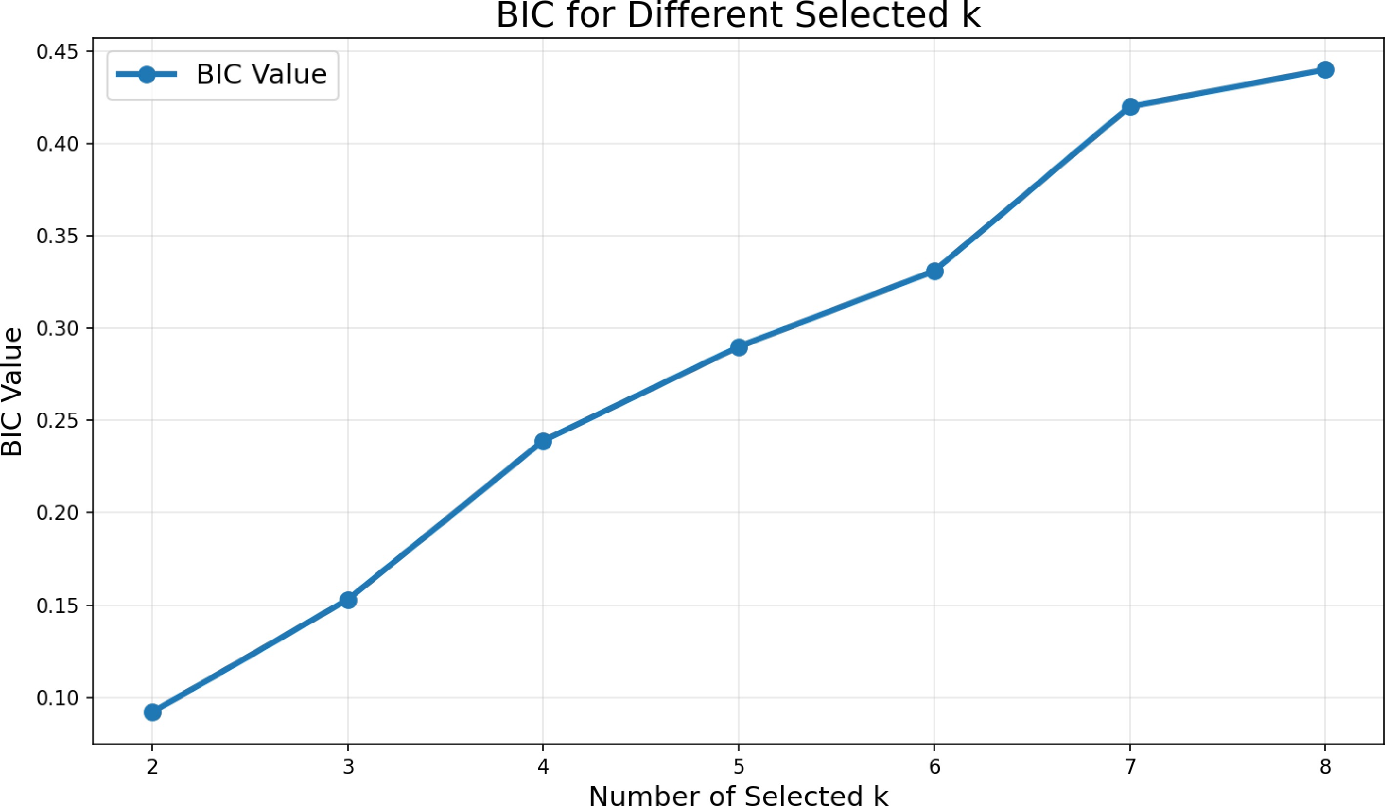
Figure 3. 

BIC values for multiple selected k.

We then randomly split the data set into training and validation sets, with 400 samples in the training set and 76 samples in the validation set. This procedure is repeated 20 times. The training data are used to fit the model, and the performance is evaluated on the validation data. We select k = 2, 3, 4 variables and compare the multistage FSA with the multistage StoIHT and IHT methods. The results are presented in Table 5.

The variable NQO1 selected by the multistage FSA method has been identified in the existing literature as the most important biomarker associated with sensitivity to 17-AAG^[47,48]. From Table 5, we observe that, across multiple choices of the selected number k, the multistage FSA achieves a smaller predicted RMSE on the validation data compared with the multistage StoIHT and IHT methods.

Madelon data set

The Madelon data set is an artificial data set designed for variable selection and classification^[49]. This data set consists of data points grouped into 32 clusters at the vertices of a five-dimensional hypercube, with labels assigned at random to +1 or −1 (relabeled as +1 or 0 in this paper). This data set contains k* = 20 informative features, including 5 original features and their 15 linear combinations. In addition, this data set includes 480 irrelevant features with no predictive power, bringing the total to 500. The data set has a sample size of 2,600. The Madelon data set is publicly available at https://archive.ics.uci.edu/dataset/171/madelon. We train shallow neural networks on the training data and report the performance on the validation data in Table 6.

We randomly split the data set into training and validation sets 20 times, with 2,000 samples in the training set and 600 samples in the validation set each time. The training data are used to fit the model, while the performance is evaluated on the validation set. We compare the performance of the proposed multistage FSA, multistage stochastic IHT, and IHT methods. In addition, the classical $ \ell_1 $-penalized method is included as a baseline for comparison. As the true number of variables is known ( k* = 20) in this data set, we use k* as the known value, and the conventional BIC and proposed HD-BIC as the criteria. For the $ \ell_1 $-penalized method, which is proposed for linear models, we use k* as the known value and the conventional BIC as the criteria. We select about 20 variables each time when k* is the known value. From Table 6, we observe that the multistage FSA outperforms the other methods across all criteria on the validation data.

This article proposes two novel stochastic algorithms for nonlinear variable selection via shallow neural networks. The first proposed algorithm is the multistage StoIHT algorithm, a stochastic version of the IHT algorithm^[31,32]. The second proposed algorithm is the multistage FSA algorithm, a variable selection method that employs an annealing strategy with the multistage StoIHT. After a comprehensive evaluation in both regression and classification settings, we conclude that the proposed multistage FSA and multistage StoIHT methods slightly outperform the IHT method in the numerical experiments presented in this paper. Furthermore, in the high-dimensional setting (large-p–small-n setting), the proposed HD-BIC outperforms the conventional BIC for variable selection. In contrast, in the low-dimensional setting (large-n–small-p setting), the conventional BIC performs better for variable selection.

Although the proposed methods exhibit strong empirical performance, they have several limitations. First, this study focuses primarily on numerical investigations, with rigorous theoretical analysis left for future research. Unlike parameter learning in linear regression, which involves only the estimation error, training a neural network model requires accounting for both estimation and approximation errors^[14]. As a result, the theoretical analysis of variable selection consistency for neural network models is substantially more complicated than that for linear regression models. Second, the present study is limited to nonlinear variable selection using shallow neural networks, and the performance of the proposed methods in the deep neural network setting remains unexplored. We will focus on these issues in our future research.