-
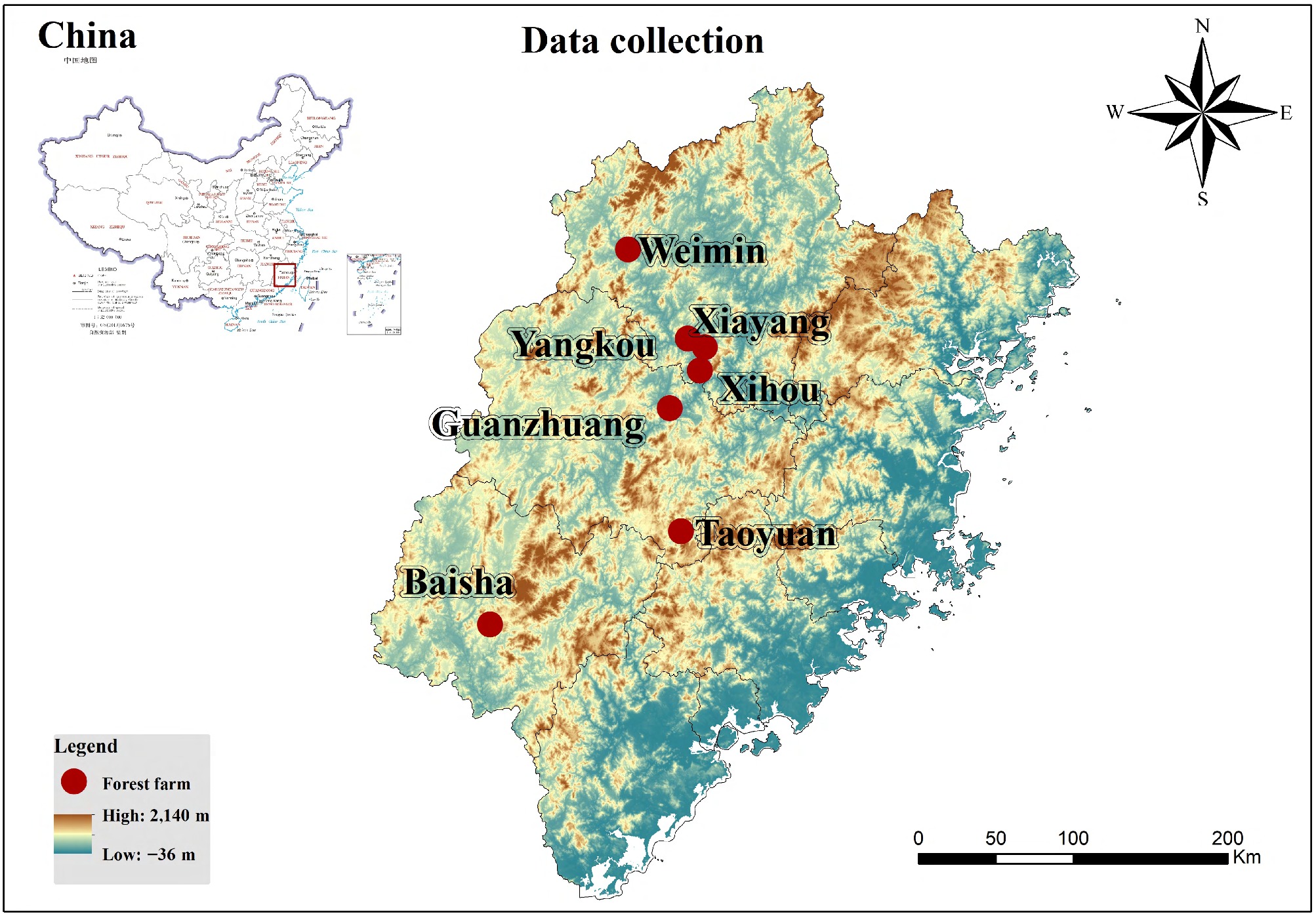
Figure 1.
Geographic locations of the seven state-owned forest farms in Fujian Province, China, where sample data were collected.
-
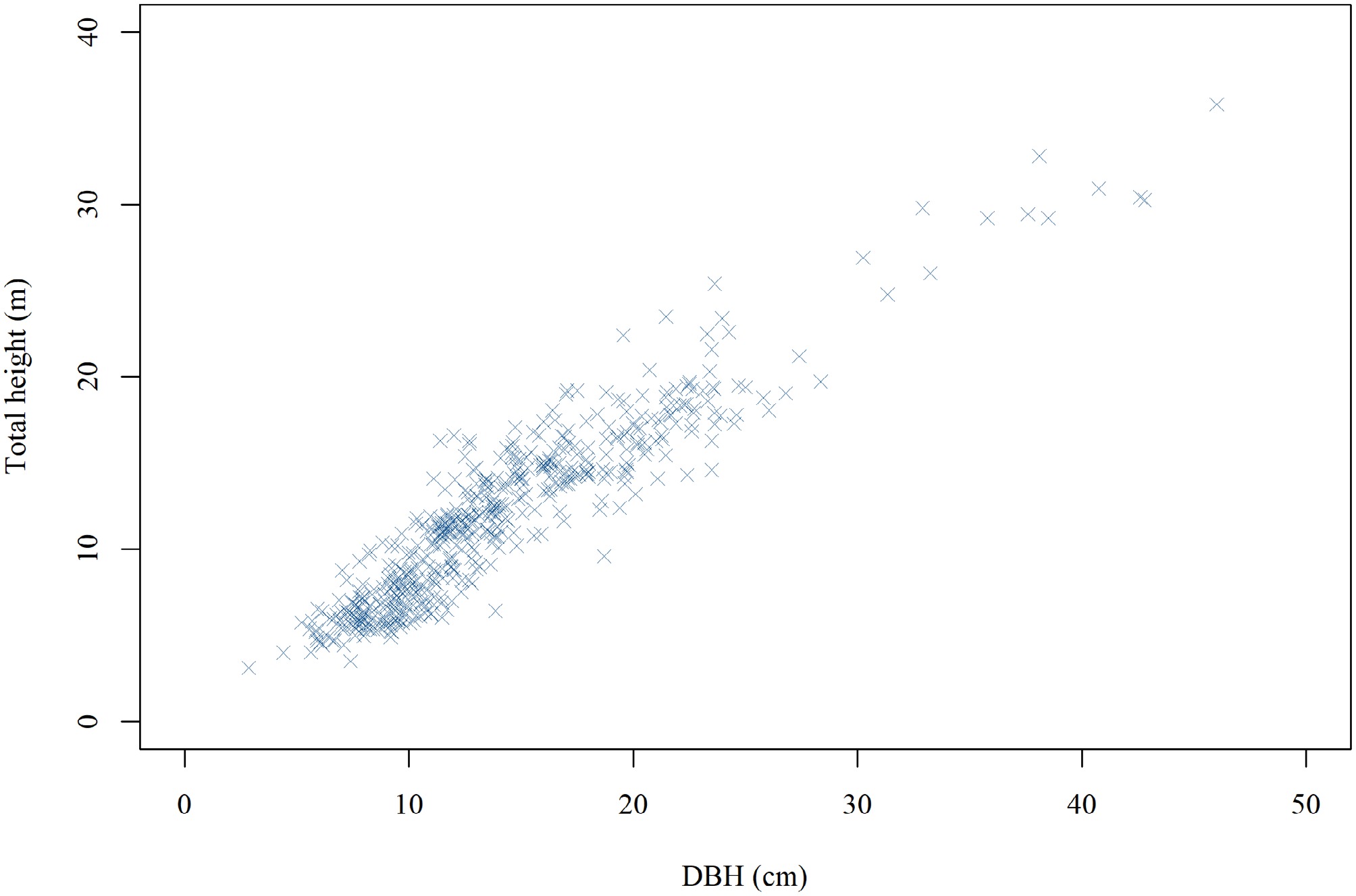
Figure 2.
Height-DBH distribution of the sampled Chinese fir trees. DBH denotes diameter at breast height.
-
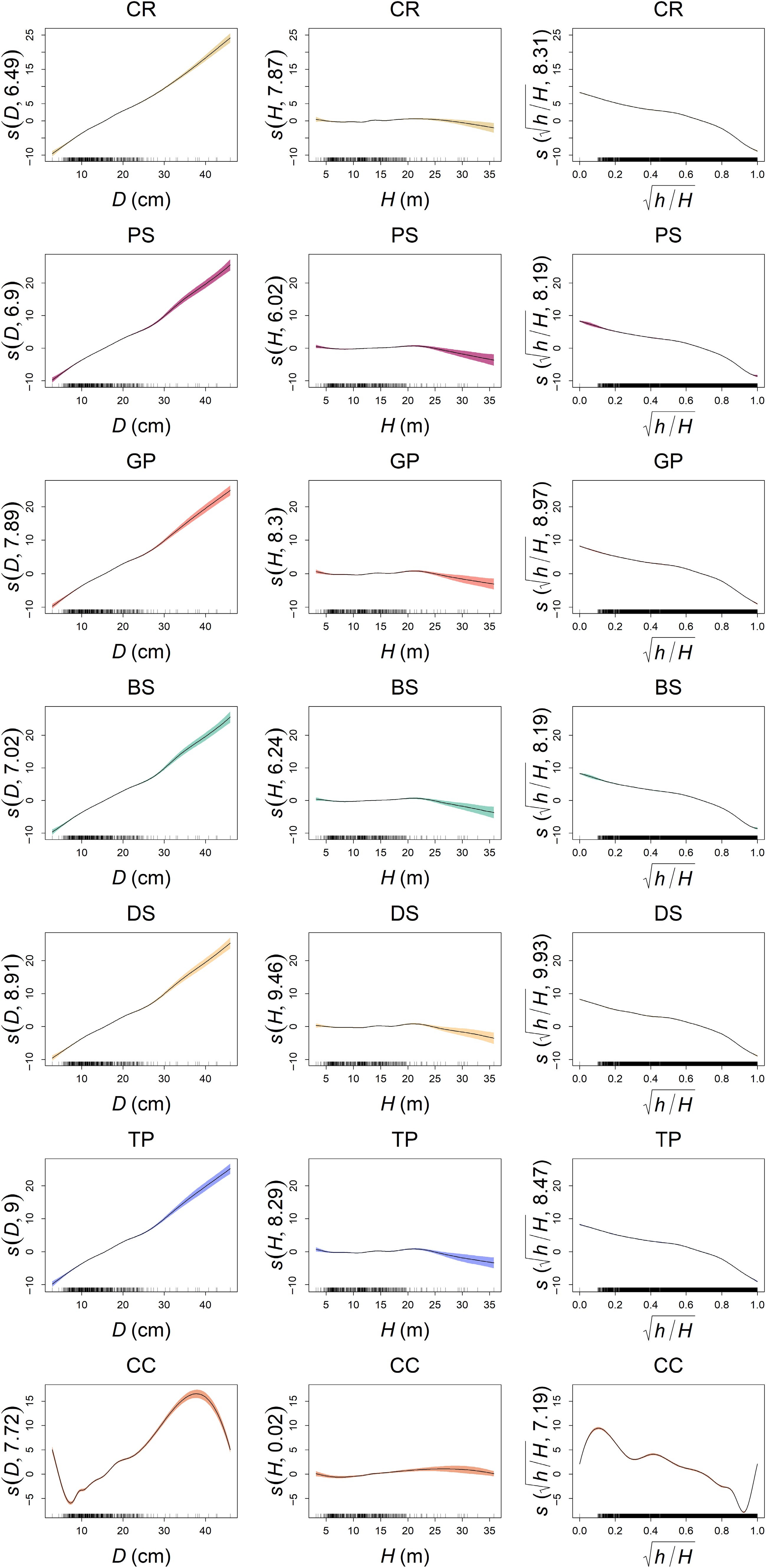
Figure 3.
Partial effects of variables for different smoothing spline functions. The numbers in parentheses on the Y-axis labels represent the estimated degrees of freedom (edf) for each smooth term, indicating the complexity of the fitted nonlinear curve.
-
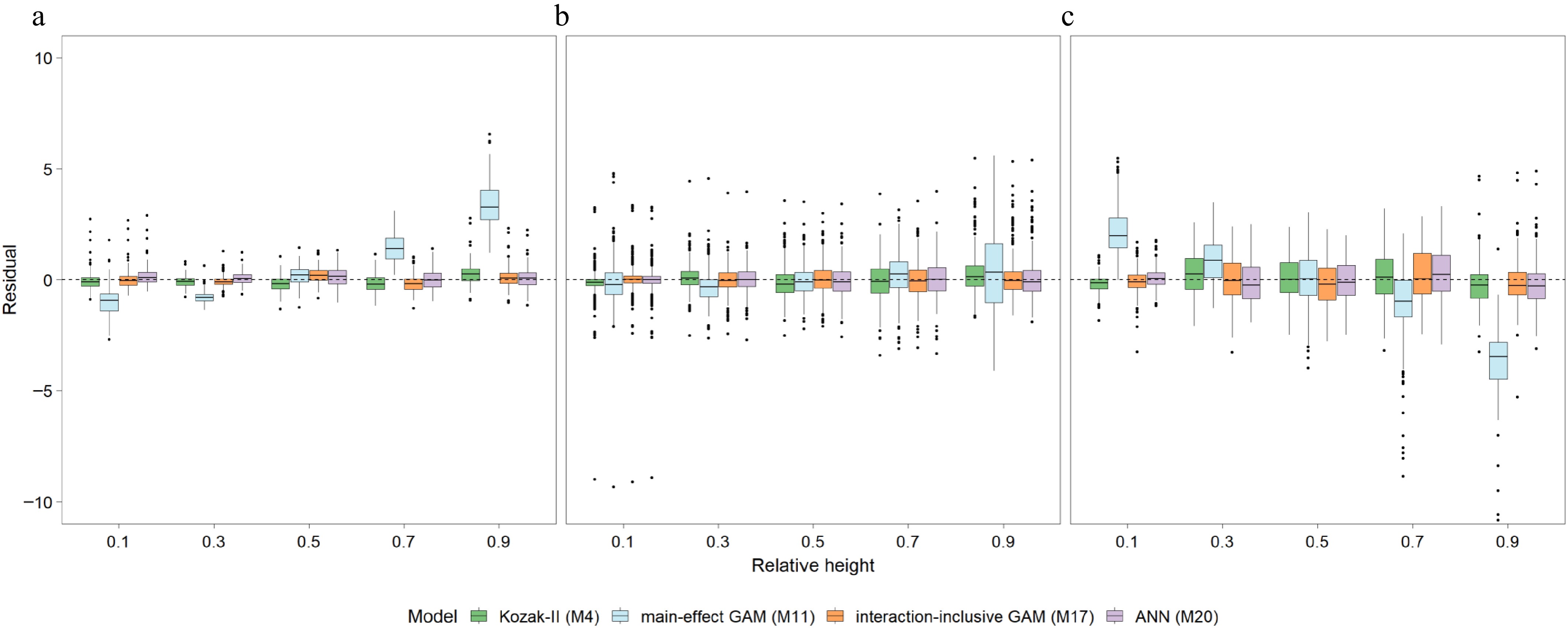
Figure 4.
Boxplots of prediction residuals across relative stem heights for (a) small (D < 10 cm), (b) medium (10 cm ≤ D < 20 cm), and (c) large trees (D ≥ 20 cm). The comparison includes the benchmark Kozak-II model (M4), the best main-effect GAM (M11), the optimal interaction-inclusive GAM (M17), and the ANN model (M20).
-
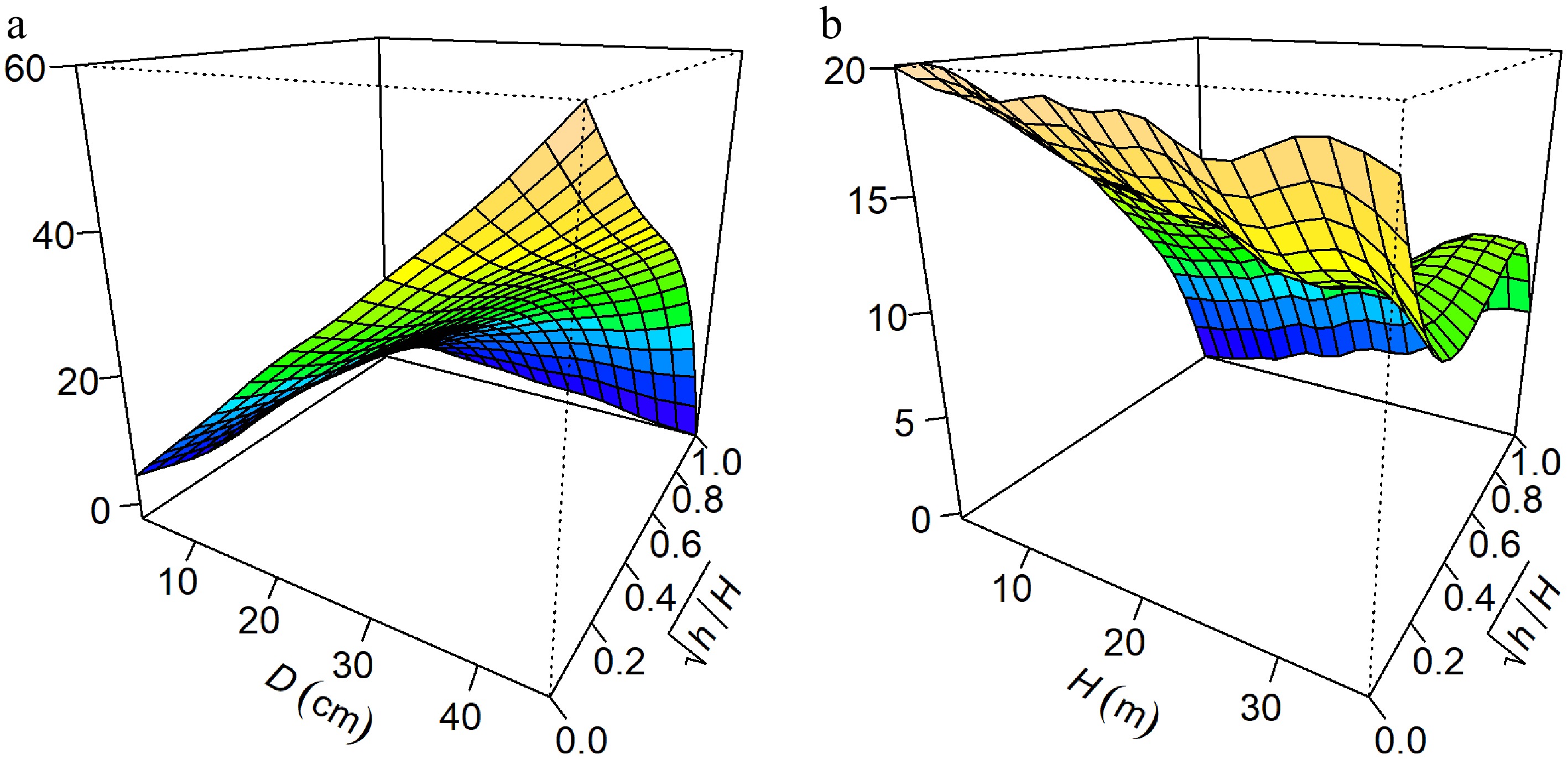
Figure 5.
Visualization of the tensor product interaction effects on predicted stem diameter from the optimal GAM (M17). The plots show the interactions between (a) D and
$ \sqrt{h/H} $ $ \sqrt{h/H} $ -
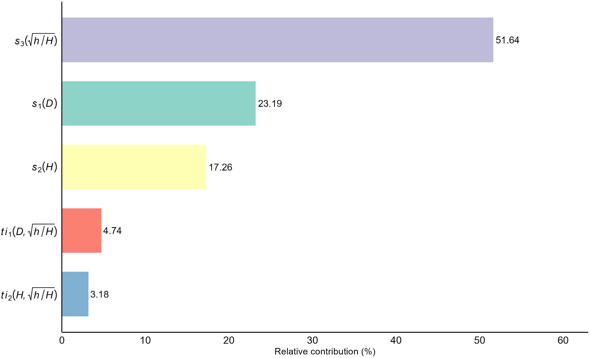
Figure 6.
Relative importance of predictors in the optimal interaction-inclusive GAM (M17), quantified as the percentage contribution of each main effect and interaction term to the total explained deviance.
-
Variable Minimum Maximum Mean SD CV (%) D (cm) 2.86 46.01 15.57 5.96 35.46 H (m) 3.13 35.80 13.34 4.85 23.50 d (cm) 0.27 63.16 11.37 6.12 37.42 h (m) 0.00 32.22 5.99 4.75 22.52 D is diameter at breast height; H is total tree height; d is stem diameter at height h; h is stem height from the butt; SD is standard deviation, CV is coefficient of variation. Table 1.
Summary statistics for the sampled Chinese fir trees.
-
Table 2.
Goodness-of-fit comparison of conventional parametric taper models for Chinese fir.
-
No. Model RMSE MAE MAPE R2 M5 $ d=\alpha +{s}_{1}\left(D\right)+{s}_{2}\left(H\right)+{s}_{3}\left(h/H\right) $ 1.8017 1.1957 19.3549 0.9132 M6 $ d=\alpha +{s}_{1}\left({D}^{2}\right)+{s}_{2}\left(H\right)+{s}_{3}\left(h/H\right) $ 1.8033 1.1960 19.3744 0.9131 M7 $ d=\alpha +{s}_{1}\left(D\right)+{s}_{2}\left(H\right)+{s}_{3}(\sqrt{h/H}) $ 1.7814 1.1798 19.3742 0.9152 M8 $ d=\alpha +{s}_{1}\left({D}^{2}\right)+{s}_{2}\left(H\right)+{s}_{3}(\sqrt{h/H}) $ 1.7830 1.1806 19.3996 0.9150 Bold numbers denote the best model for each criterion. Table 3.
Comparison of goodness-of-fit statistics for main-effect GAMs using different variable transformations.
-
No. Spline function RMSE MAE MAPE R2 M9 BS 1.7830 1.1793 19.3216 0.9150 M10 PS 1.7831 1.1794 19.3263 0.9150 M11 DS 1.7789 1.1768 19.3203 0.9154 M12 TP 1.7814 1.1798 19.3742 0.9152 M13 GP 1.7804 1.1789 19.3737 0.9153 M14 CR 1.7825 1.1797 19.3603 0.9151 M15 CC 2.9298 1.7361 31.5170 0.7706 Bold numbers denote the best model for each criterion. Table 4.
Comparison of goodness-of-fit statistics for main-effect GAMs constructed with different smoothing spline functions.
-
No. RMSE MAE MAPE R2 M1 1.0192 0.6340 7.6203 0.9719 M2 1.0456 0.7345 8.6664 0.9704 M3 1.0866 0.7955 10.9481 0.9681 M4 0.8746 0.5828 7.1727 0.9793 M9 1.8058 1.1945 19.5991 0.9127 M10 1.8065 1.1952 19.6147 0.9126 M11 1.8045 1.1945 19.5934 0.9130 M12 1.8027 1.1954 19.6199 0.9130 M13 1.8021 1.1945 19.6288 0.9130 M14 1.8016 1.1945 19.6139 0.9131 M15 3.0705 1.7842 32.0782 0.7421 Bold numbers denote the best model for each criterion. Table 5.
Cross-validation statistics for parametric and main-effect additive taper models.
-
No. Model Spline function RMSE MAE MAPE R2 M16 $ d=\alpha +{s}_{1}\left(D\right)+{s}_{2}\left(H\right)+{s}_{3}\left(\sqrt{h/H}\right)+{ti}_{1}\left(D,\sqrt{h/H}\right) $ GP 0.8534 0.5776 7.2471 0.9805 M17 $ d=\alpha +{s}_{1}\left(D\right)+{s}_{2}\left(H\right)+{s}_{3}\left(\sqrt{h/H}\right)+{ti}_{1}(D,\sqrt{h/H})+{ti}_{2}(H,\sqrt{h/H}) $ DS 0.8212 0.5404 6.6636 0.9820 M18 $ d=\alpha +{s}_{1}\left(D\right)+{s}_{2}\left(H\right)+{s}_{3}\left(\sqrt{h/H}\right)+{ti}_{1}\left(D,H\right)+{ti}_{2}\left(D,\sqrt{h/H}\right)+{ti}_{3}(H,\sqrt{h/H}) $
BS 0.8129 0.5365 6.6722 0.9823 M19 $ d=\alpha +{s}_{1}\left(D\right)+{s}_{2}\left(H\right)+{s}_{3}\left(\sqrt{h/H}\right)+{ti}_{1}\left(D,H,\sqrt{h/H}\right) $ BS 0.8316 0.5512 6.8612 0.9815 Bold numbers denote the best model for each criterion. Table 6.
Performance comparison of the best-performing GAMs with varying levels of interaction complexity.
-
No. Model RMSE MAE MAPE R2 M4 Kozak-II 0.8746 0.5828 7.1727 0.9793 M11 $ d=\alpha +{s}_{1}\left(D\right)+{s}_{2}\left(H\right)+{s}_{3}(\sqrt{h/H}) $ 1.8045 1.1956 19.5934 0.9128 M16 $ d=\alpha +{s}_{1}\left(D\right)+{s}_{2}\left(H\right)+{s}_{3}\left(\sqrt{h/H}\right)+{ti}_{1}\left(D,\sqrt{h/H}\right) $ 0.8864 0.6003 7.5216 0.9787 M17 $ d=\alpha +{s}_{1}\left(D\right)+{s}_{2}\left(H\right)+{s}_{3}\left(\sqrt{h/H}\right)+{ti}_{1}(D,\sqrt{h/H})+{ti}_{2}(H,\sqrt{h/H}) $ 0.8688 0.5765 7.0451 0.9796 M18 $ d=\alpha +{s}_{1}\left(D\right)+{s}_{2}\left(H\right)+{s}_{3}\left(\sqrt{h/H}\right)+{ti}_{1}\left(D,H\right)+{ti}_{2}\left(D,\sqrt{h/H}\right)+{ti}_{3}(H,\sqrt{h/H}) $
0.8965 0.5791 7.0870 0.9783 M19 $ d=\alpha +{s}_{1}\left(D\right)+{s}_{2}\left(H\right)+{s}_{3}\left(\sqrt{h/H}\right)+{ti}_{1}\left(D,H,\sqrt{h/H}\right) $ 1.2807 0.6148 7.4740 0.9441 M20 Artificial Neural Networks (ANN) 0.8742 0.5836 7.2455 0.9793 M21 Random Forest (RF) 1.1009 0.7289 9.3892 0.9673 Bold numbers denote the best model for each criterion. Table 7.
Cross-validation performance metrics comparing the interaction-inclusive GAMs against parametric and machine learning benchmarks.
-
Term Estimate (SE) edf Ref.df p-value Intercept 11.458 (0.008) < 0.001 $ {s}_{1}(D) $ 9.593 10.57 < 0.001 $ {s}_{2}(H) $ 10.660 10.95 < 0.001 $ {s}_{3}(\sqrt{h/H}) $ 10.557 10.95 < 0.001 $ {ti}_{1}(D,\sqrt{h/H}) $ 13.454 14.87 < 0.001 $ {ti}_{2}(H,\sqrt{h/H}) $ 13.955 15.32 < 0.001 SE denotes standard error; edf and Ref.df are effective degrees of freedom and reference degrees of freedom respectively. Table 8.
Parameter estimates and smooth term statistics of the optimal interaction-inclusive GAM (M17).
Figures
(6)
Tables
(8)