Tree size and relative height interactions enhance generalized additive models for Chinese fir stem taper prediction

Sustainable forest management and the precise estimation of carbon stocks rely fundamentally on the accurate quantification of timber resources^[1,2]. While stem taper models serve as indispensable tools for these tasks by describing the gradual decrease in stem diameter with increasing height^[3,4], stem taper is not a static geometric attribute. Instead, it represents a dynamic phenotype that evolves with tree ontogeny. According to the constant stress hypothesis and metabolic scaling theories, trees allocate biomass along the stem to equalize the distribution of bending stress caused by wind loading and self-weight^[5−8]. As a tree matures and increases in size, its stem form factor must evolve to maintain stability. For instance, larger dominant trees typically develop a more pronounced basal flare to resist higher bending moments compared to smaller subdominant individuals^[9]. This allometric scaling implies that the taper profile is inextricably dependent on the absolute size of the tree. Therefore, accurate taper models must account for this nonlinear interplay between tree size and relative position along the stem to capture the inherent biological plasticity of tree form.

The quest for taper modeling boasts a rich history spanning over a century with seminal contributions from researchers like Larson^[5], Newnham^[10], and notably Kozak^[11,12], whose variable-exponent models represent a widely adopted benchmark in forest inventory^[13−17]. These traditional parametric approaches possess inherent advantages regarding interpretability as their parameters often carry direct biological meanings that can be incorporated into hierarchical modeling frameworks^[18−20]. However, their reliance on predefined mathematical forms imposes a limitation. Specifically, such structural constraints can restrict flexibility in capturing the inherent variability and complex shapes of tree stems, especially under diverse site conditions or for trees exhibiting irregular growth patterns^[21,22]. This inherent rigidity has motivated the exploration of more adaptable modeling frameworks.

Generalized additive models (GAMs) offer a compelling alternative by blending the interpretability of linear models with the flexibility of nonparametric smoothing functions to capture complex data-driven relationships without stringent a priori assumptions^[23,24]. While pioneering studies^{[21,22,25,26]} successfully established the viability of GAMs in taper modeling, they primarily focused on capturing the additive effects of key predictors independently. This additive assumption overlooks the critical interaction effects where the influence of relative height on taper varies significantly depending on tree size. Although recent machine learning algorithms like artificial neural networks (ANN) and random forest (RF) can effectively capture such complex nonlinearities^[22,27], these methods often operate as black boxes that prioritize predictive accuracy at the expense of biological interpretability^[28,29]. Consequently, there is a lack of modeling frameworks that can bridge this gap by offering the predictive power of machine learning regarding interaction effects while retaining the inferential transparency of parametric models. While GAMs have shown promise, the application of interaction-inclusive models utilizing tensor product smooths^[30] to resolve this modeling trade-off remains underexplored.

In this study, we address this knowledge gap using Chinese fir (Cunninghamia lanceolata) as a model species. As the most extensively planted species in Southern China with paramount economic and ecological significance^[31−33], Chinese fir exhibits rapid growth and significant morphological variation, making it an ideal candidate for examining size-dependent taper dynamics. We address the limitations of previous methods by developing GAM-based taper models that explicitly incorporate interaction effects of varying complexity. Our primary objective is to construct GAMs incorporating tensor product interactions to identify the optimal structure for stem taper prediction. We subsequently evaluate the performance of these models against established parametric equations and popular machine learning algorithms while quantifying the relative contributions of main and interactive effects. Ultimately, we aim to connect these statistical interaction patterns with the biological principles governing size-dependent stem form development.

The stem form data for this study were collected from Fujian Province in Southeastern China, a region renowned for its production of high-quality Chinese fir timber. The province is characterized by a high forest coverage rate of 65.12%, an extensive mountainous landscape, and a humid, rainy climate throughout the year. These environmental conditions provide an ideal natural habitat for the robust growth of Chinese fir.

Data were sourced from seven state-owned forest farms strategically located across the province including Guanzhuang (117°35'−117°50' E, 26°24'−27°38' N), Taoyuan (117°32'−117°48' E, 25°15'−25°22' N), Baisha (116°30'−116°38' E, 25°04'−25°15' N), Xihou (118°02'−118°13' E, 26°36'−26°47' N), Yangkou (117°46'−118°25' E, 26°28'−26°54' N), Weimin (117°48'−117°51' E, 26°56'−26°57' N), and Xiayang (117°54'−118°02' E, 26°44'−26°52' N). Figure 1 shows the specific locations of each forest farm.

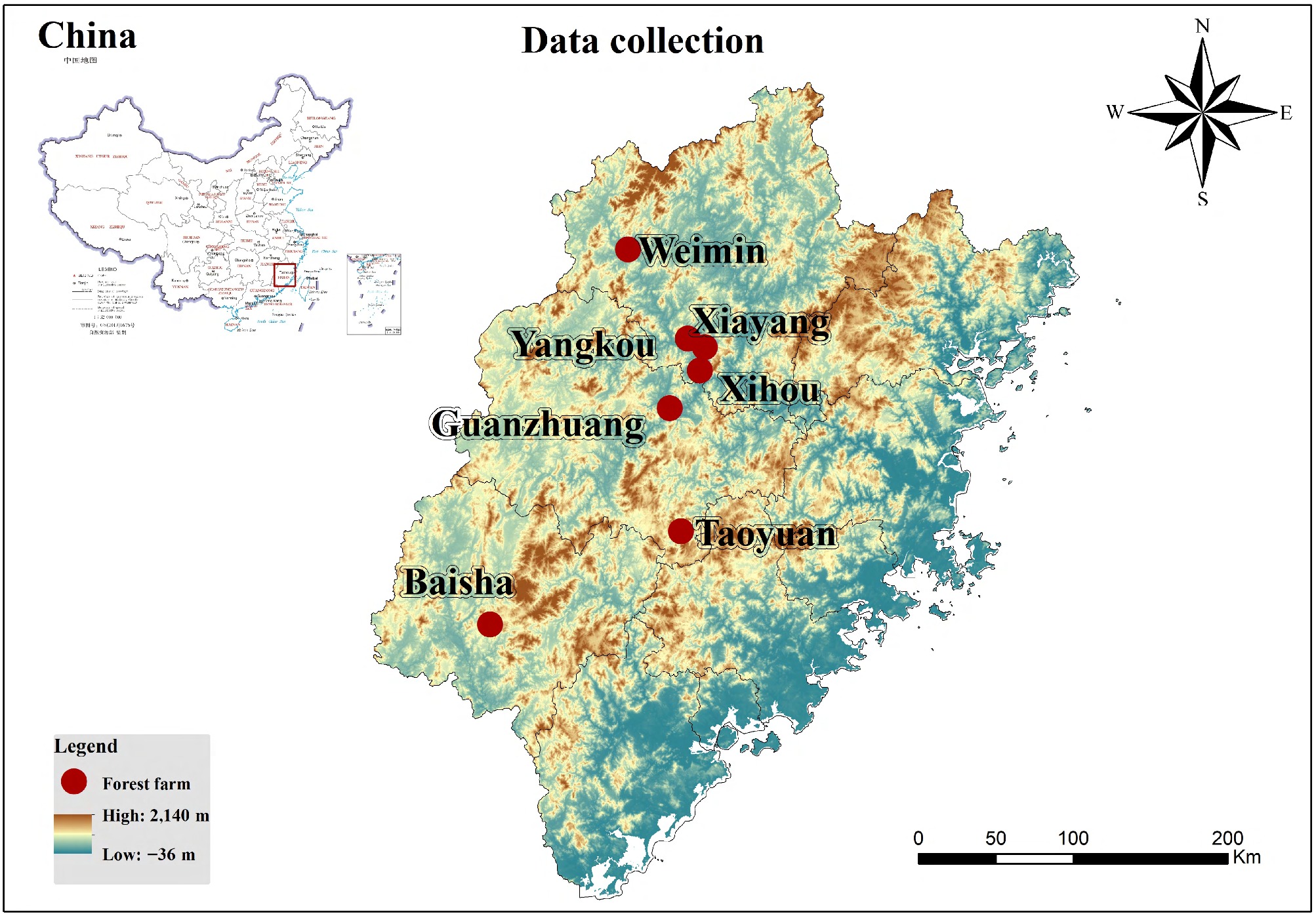
Figure 1. 

Geographic locations of the seven state-owned forest farms in Fujian Province, China, where sample data were collected.

For each sample tree felled, the tree age and an identification number were recorded. The DBH and total tree height (H) were then measured. Following this, the stem diameter was systematically measured at multiple predetermined positions along the bole starting from the base (0 m) and continuing at relative heights of 0.02, 0.04, 0.06, 0.08, 0.1, 0.15, 0.2, 0.25, 0.3, 0.4, 0.5, 0.6, 0.7, 0.75, 0.8, 0.9, and 0.95 H. In total, 516 felled Chinese fir trees were measured, yielding 10,374 individual diameter observations. Summary statistics for these measurements are presented in Table 1, while Fig. 2 illustrates the height-DBH distribution for the entire dataset.

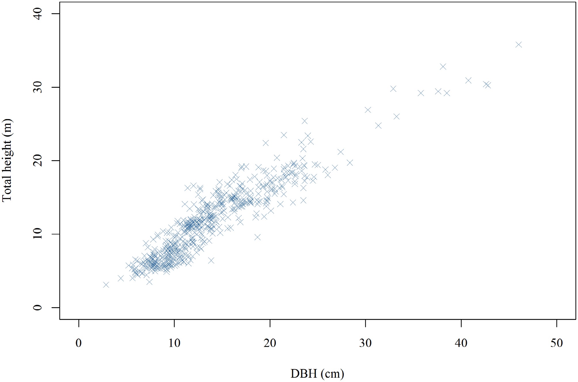
Figure 2. 

Height-DBH distribution of the sampled Chinese fir trees. DBH denotes diameter at breast height.

Conventional parametric taper models

To identify a benchmark for performance, we first fitted the Chinese fir stem profile data using four widely recognized variable-exponent taper equations. These models, selected for their frequent application and proven utility in forest inventory, were the Zeng & Liao^[34] model, the Lee^[35] model, and two variants of the Kozak^[12] model, herein referred to as Kozak-I and Kozak-II. The mathematical forms of these models are as follows:

where, d represents the diameter at various stem positions (cm); h denotes the height at those positions (m); D is the diameter at breast height (DBH, cm); H indicates total tree height (m); h/H signifies relative height; a₀, a₁, a₂, a₃, a₄, a₅, a₆, a₇, and a₈ are model parameters; and ε is the random error term.

Generalized additive taper models

The fundamental mathematical expression for a generalized additive model (GAM) is:

where, Y is the response variable; α is the intercept; x₁, …, x_m are the explanatory variables; s(·) denotes a nonparametric smoothing spline function for each variable; and m is the number of predictors.

To ensure a fair and direct comparison with the parametric models, we maintained the same variable selection in developing the GAM-based taper models. We designated the stem diameter at a given height (d) as the response variable, with DBH (D), total tree height (H), and relative height (h/H) serving as the explanatory variables. To determine the most appropriate model structure, we formulated and compared four distinct GAMs based on different variable transformations^[36]:

To examine the influence of different spline functions on GAM performance, we constructed models using seven distinct types of splines after identifying the optimal model structure from Eqs. (6)−(9). The evaluated splines included basis spline (BS), penalized B-spline (PS), Duchon spline (DS), thin plate spline (TP), Gaussian process spline (GP), cubic regression spline (CR), and cubic cyclic spline (CC). All GAMs were fitted using the restricted maximum-likelihood (REML) method. This approach was chosen over standard maximum likelihood (ML) to mitigate the potential for downward bias in variance component estimation, thereby enhancing model stability.

A key strength of GAMs lies in their capacity to effectively model complex, nonlinear interactions between variables. We explored these interactions using tensor product interaction smooths, which allow for the explicit separation of interaction effects from the main effects of the predictors. To identify the optimal trade-off between model complexity and predictive power, we constructed a series of candidate GAMs incorporating different combinations of interaction terms based on the optimal main-effect structure. Taking Eq. (6) as a base example, a GAM incorporating all two-way interactions would take the following form:

where, ti(·) denotes the tensor product interaction smooth function.

Machine learning models

To provide a comprehensive benchmark for the proposed GAMs, we developed two widely used machine learning models: artificial neural networks (ANN) and random forest (RF). Both models utilized the same predictors as the GAMs (D, H, and relative height terms) to ensure comparability.

The ANN model was constructed using a multilayer perceptron architecture with the neuralnet package in R^[37]. We employed a resilient backpropagation algorithm with a single hidden layer. To determine the optimal network architecture, we performed a grid search for the number of neurons in the hidden layer (ranging from 1 to 10), selecting the configuration that minimized the mean square error in the cross-validation. Based on this grid search, the optimal network architecture was established as a single hidden layer with three neurons.

The RF model was implemented using the randomForest package^[38]. We optimized two key hyperparameters: the number of trees (ntree) and the number of variables randomly sampled at each split (mtry). The optimal hyperparameter combination was identified by evaluating the out-of-bag error and cross-validation performance across a range of candidate values. Consequently, the final hyperparameters were set to 1,000 for the number of trees and 2 for the number of variables randomly sampled at each split.

Model evaluation

The performance of all taper models was evaluated using a five-fold cross-validation procedure based on tree ID. The entire dataset of 516 trees was randomly partitioned into five mutually exclusive subsets. In an iterative process, four subsets were combined for model training, and the remaining one was used for validation. This process was repeated five times until every tree had served as a validation sample exactly once. The final model performance was assessed by averaging the evaluation metrics from the five validation folds.

To ensure statistical validity, the selection of evaluation criteria depended on the specific modeling context. We employed Akaike's information criterion (AIC), Bayesian information criterion (BIC), and −2*log-likelihood (−2LogLik) exclusively for the internal performance assessment of the four candidate parametric models. Lower values for these indices signify a superior fit. For all other model evaluations, we relied on standard predictive metrics for both model fitting and cross-validation. These metrics comprised the root mean square error (RMSE), mean absolute error (MAE), mean absolute percentage error (MAPE), and fit index (R²). Superior predictive performance is indicated by lower values of RMSE, MAE, and MAPE, and a higher value of R². The formulas for these statistical indicators are as follows:

where, k is the number of model parameters; n is the sample size; L is the likelihood function; d_i and $ {\hat{d}}_{i} $ are the i^th observed and predicted stem diameter; and $ \bar{d} $ is the mean of the observed stem diameters.

Variable importance analysis

Based on the optimal GAM taper equation, the relative importance of each predictor and their interaction terms was quantified using the gam.hp package in R^[39]. This approach implements hierarchical partitioning to decompose the total explained deviance into components attributable to each predictor's independent contribution, thereby providing robust importance estimates even in the presence of multicollinearity.

Our baseline analysis demonstrated that conventional parametric models establish a stringent benchmark for predictive accuracy. Among the four variable-exponent candidates (M1−M4), the Kozak-II model (M4) demonstrated the superior goodness-of-fit, yielding the lowest AIC, BIC, and −2LogLik values (Table 2). In contrast, generalized additive models constructed solely with main effects proved insufficient to capture the full complexity of taper dynamics. Although the screening of predictor functional forms (Table 3) and smoothing splines (Table 4) identified the Duchon spline model incorporating D, H, and $ \sqrt{h/H} $ (M11) as the optimal additive structure, it failed to surpass the predictive accuracy of the parametric benchmark (Table 5).

The partial effects of the predictors derived from these main-effect GAMs are visualized in Fig. 3. Consistent patterns emerged across all spline types except CC. Specifically, the predicted stem diameter (d) exhibited a gradual nonlinear increase with D alongside widening confidence intervals. The relationship between d and H remained relatively stable but demonstrated greater uncertainty at larger heights. Additionally, d displayed a pronounced nonlinear decline with increasing $ \sqrt{h/H} $ 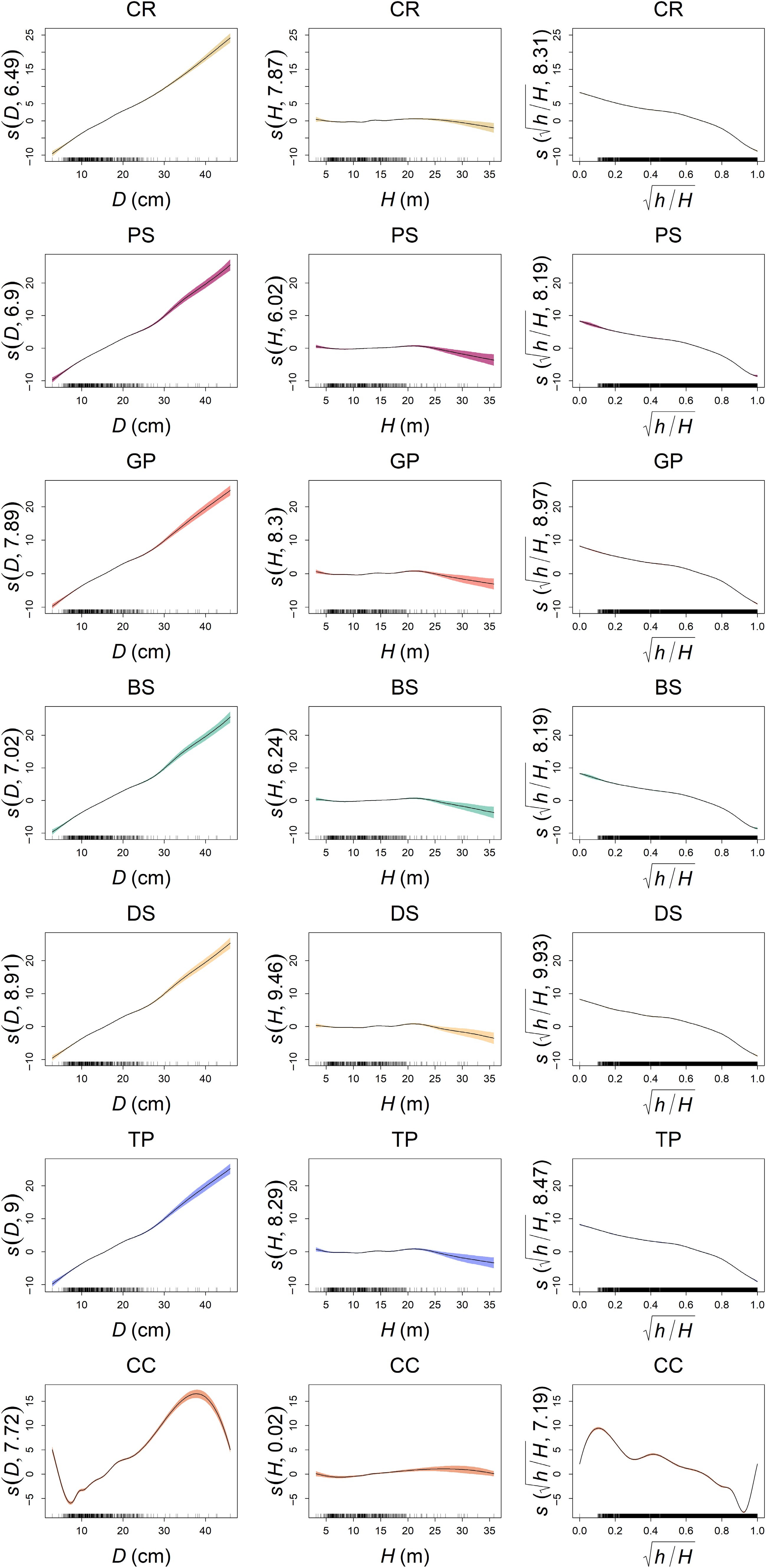while maintaining narrow and stable confidence intervals.

Figure 3. 

Partial effects of variables for different smoothing spline functions. The numbers in parentheses on the Y-axis labels represent the estimated degrees of freedom (edf) for each smooth term, indicating the complexity of the fitted nonlinear curve.

Performance enhancement via interaction terms

Explicitly modeling tensor product interactions overcame the structural limitations of additive frameworks and yielded significant performance gains. Seventy-seven GAMs with distinct two-way and three-way interaction structures across various spline functions were examined, and the four best-performing GAMs representing varying levels of interaction complexity are presented in Table 6. The inclusion of interaction terms substantially reduced fitting errors, where the model incorporating all two-way interactions (M18) achieved the highest fitting performance. Meanwhile, the model with two interactions (M17 excluding the D and H interaction) demonstrated comparable accuracy.

However, the five-fold cross-validation results summarized in Table 7 highlighted a critical trade-off between complexity and generalization. The more parsimonious model (M17), which incorporates only two specific interaction terms $ {ti}_{1}(D,\sqrt{h/H}) $ and $ {ti}_{2}(H,\sqrt{h/H}) $, demonstrated the best generalization capability among all representative models. M17 yielded the lowest validation RMSE (0.8688 cm), MAE (0.5765 cm), MAPE (7.05%), and the highest R² (0.9796), outperforming both the complex M18 and the parametric benchmark (M4). Crucially, this interaction-inclusive GAM (M17) also demonstrated superior predictive power compared to the black-box machine learning algorithms, surpassing both the artificial neural network (M20) and random forest (M21) benchmarks.

The detailed parameter statistics based on the entire dataset for the optimal M17 model are provided in Table 8. As shown, all main effect and interaction smooth terms exhibited estimated degrees of freedom (edf) substantially greater than 1. This statistically confirms the highly nonlinear nature of these biological relationships, with higher edf values reflecting the complex, flexible curve structures required to accurately model the taper profile.

Statistical interpretation and bias correction

Stratified residual analysis (Fig. 4) elucidated the source of this predictive superiority. The main-effect GAM (M11) exhibited systematic bias characterized by the overestimation of top diameters in small trees (D < 10 cm) and underestimation in large trees (D ≥ 20 cm). In contrast, the optimal interaction-inclusive model (M17) effectively corrected these size-dependent structural deviations, maintaining homogeneous residuals centered near zero. Notably, M17 demonstrated superior stability with slightly tighter residual distributions compared to both the benchmark Kozak-II model (M4) and the ANN model (M20), confirming its robust predictive capability across all tree sizes and stem heights.

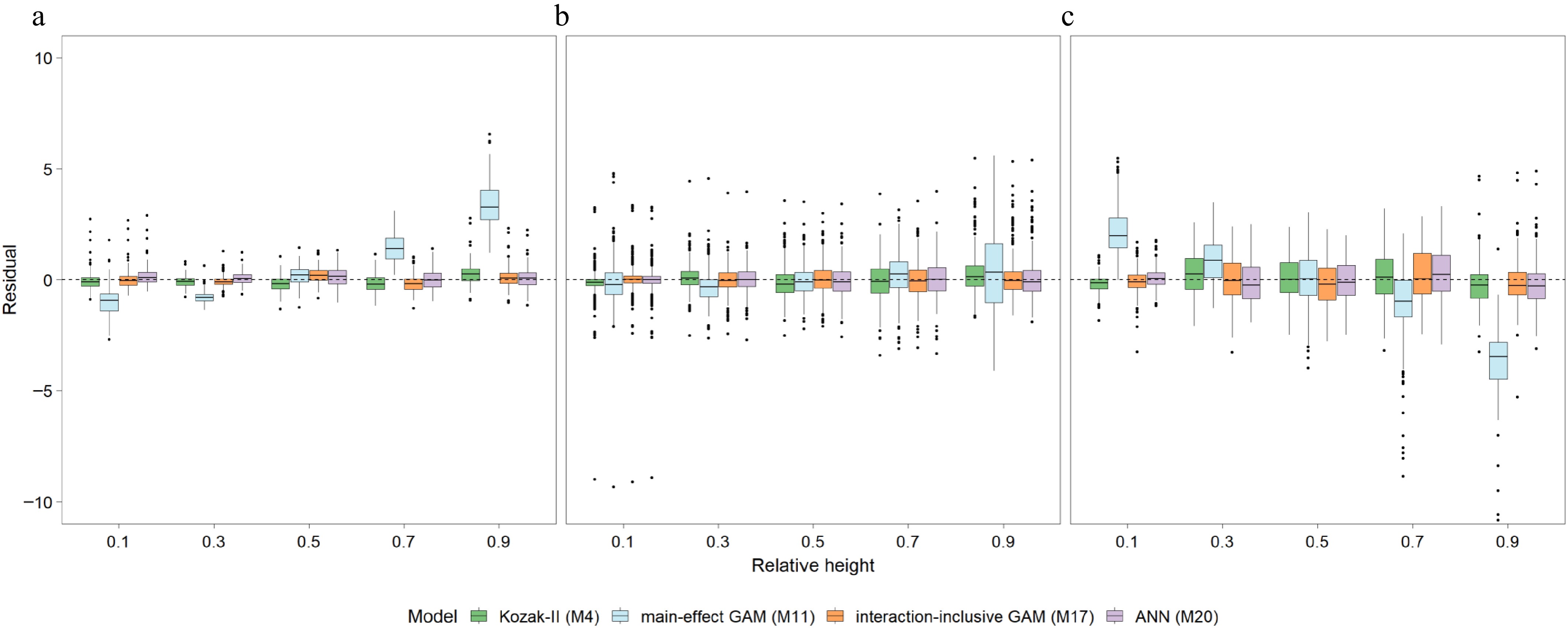
Figure 4. 

Boxplots of prediction residuals across relative stem heights for (a) small (D < 10 cm), (b) medium (10 cm ≤ D < 20 cm), and (c) large trees (D ≥ 20 cm). The comparison includes the benchmark Kozak-II model (M4), the best main-effect GAM (M11), the optimal interaction-inclusive GAM (M17), and the ANN model (M20).

The statistical basis for this correction is illustrated in the three-dimensional visualization of tensor product surfaces (Fig. 5). The interaction between DBH and $ \sqrt{h/H} $ manifested as a steep, nonlinear surge in predicted diameter at the stem base specifically for large-diameter trees (Fig. 5a), accurately capturing the biological phenomenon of basal flare. Meanwhile, the interaction between total height and $ \sqrt{h/H} $ (Fig. 5b) was primarily concentrated in the lower stem section across the entire range of tree heights. Unlike the dominant DBH interaction, this surface displayed a significantly lower z-axis range and a more subtle curvature, indicating that total height exerts a continuous but moderate influence on the stem taper profile, serving as a modifying factor rather than a primary driver of diameter magnitude.

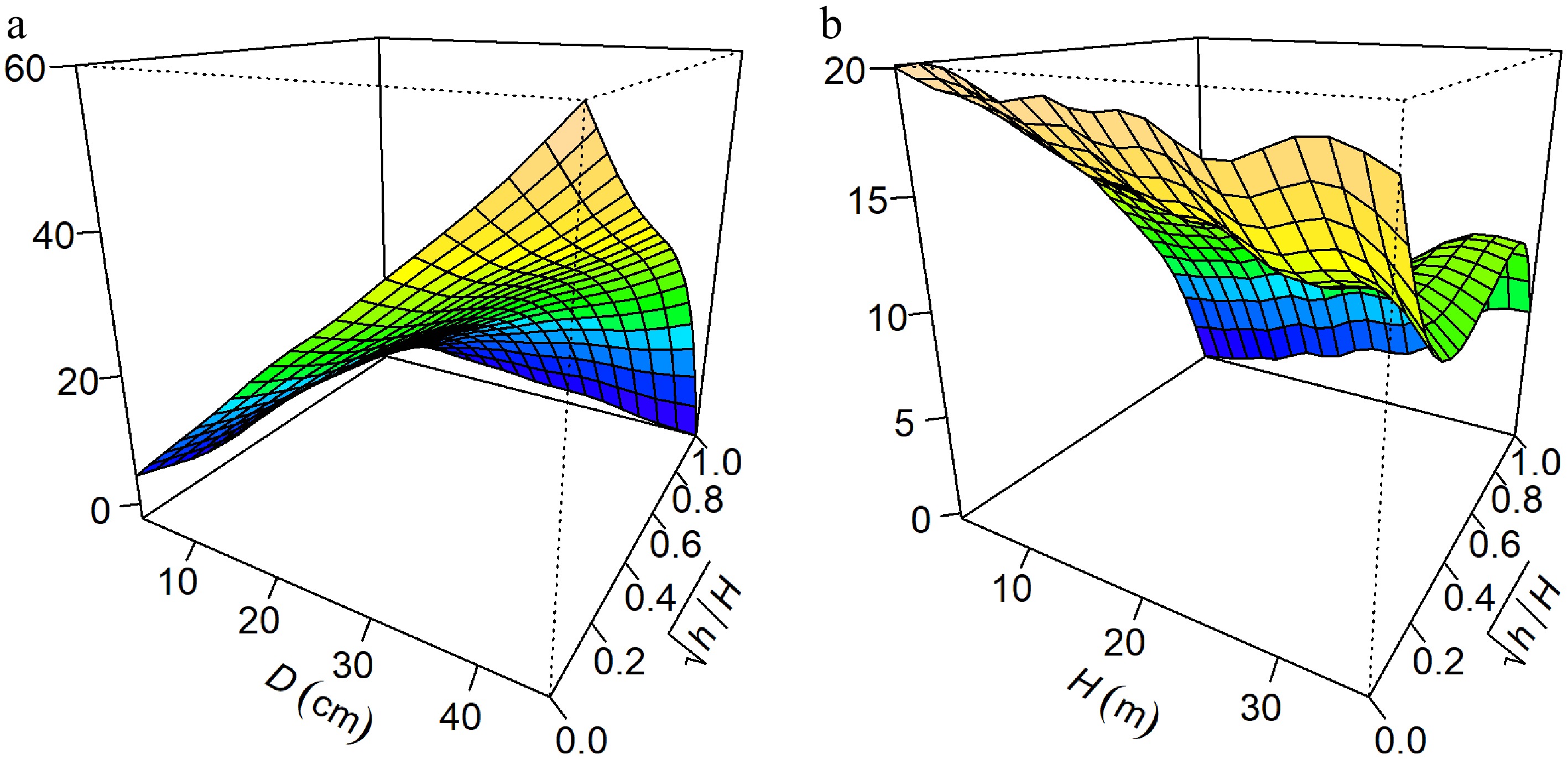
Figure 5. 

Visualization of the tensor product interaction effects on predicted stem diameter from the optimal GAM (M17). The plots show the interactions between (a) D and $ \sqrt{h/H} $, and (b) H and $ \sqrt{h/H} $. The warping of the surface plane indicates the magnitude of the interaction effect.

Variable importance analysis (Fig. 6) quantified this architectural hierarchy. While the square root of relative height ($ \sqrt{h/H} $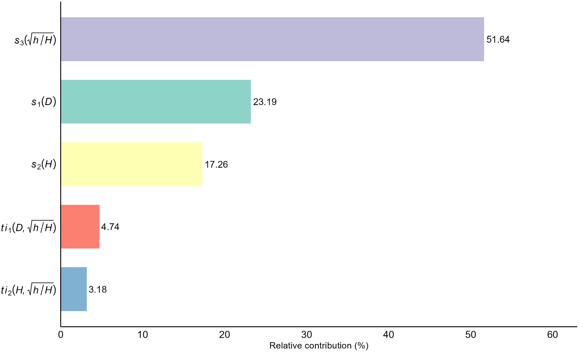) remained the dominant predictor (51.64%), the interaction terms collectively accounted for 7.92% of the total explained deviance, acting as the critical modifiers that fine-tune stem form predictions beyond the capacity of main effects.

Figure 6. 

Relative importance of predictors in the optimal interaction-inclusive GAM (M17), quantified as the percentage contribution of each main effect and interaction term to the total explained deviance.

This study demonstrates that the incorporation of interaction effects into generalized additive models substantially enhances stem taper prediction for Chinese fir, yielding results that outperform both conventional parametric equations and main-effect GAMs. While previous studies have established the viability of GAMs for taper modeling^[21,25,26], they predominantly relied on additive structures. Our results reveal a critical limitation of this approach, as the best-performing main-effect GAM was inferior to the benchmark Kozak-II model (Table 7). This seemingly counterintuitive finding underscores that the Kozak model, through its multiplicative structure and complex exponents, implicitly captures the interactive nature of stem tapering. A purely additive GAM fails to account for these synergies and consequently provides a biased representation of the underlying biological process. While traditional parametric models can also be refined by manually incorporating multiplicative or divisive interaction terms to improve performance, such modifications often rely on a priori assumptions or iterative trial and error to determine the correct functional form for a specific dataset. In contrast, the true power of the GAM framework was realized when we explicitly modeled these interactions using tensor product smooths, which allows for the automatic discovery of optimal interaction structures in a data-driven manner. The optimal interaction-inclusive model M17 reduced the cross-validation RMSE by 52.3% relative to the main-effect model M11. More importantly, it demonstrated robust predictive capacity by outperforming the rigorous Kozak-II parametric benchmark while offering superior residual homogeneity across all tree sizes (Fig. 4).

A key contribution of this study is the rigorous selection of the interaction structure based on predictive generalization rather than simple goodness of fit. Although the model with three two-way interactions (M18) achieved the best fit on the training data, the cross-validation results favored the simpler model with two interactions (M17). M17 yielded the lowest predictive errors in the validation phase (Table 7), suggesting that the additional interaction term between DBH and total height in M18 introduced redundancy or overfitting. This aligns with the principle of parsimony in statistical modeling^[40]. The interaction between DBH and total height likely captured sample-specific noise rather than a general biological trend, whereas the interactions involving relative height are essential for defining the stem profile. Consequently, we recommend M17 as the optimal model since it strikes the best balance between model complexity and predictive robustness.

Furthermore, our comparison with machine learning approaches highlights a significant advantage of the interaction-inclusive GAM. While the artificial neural network (M20) achieved high accuracy comparable to the parametric benchmark, it functions as a black box where functional relationships are obscured^[28,29]. In contrast, M17 not only outperformed both artificial neural networks and random forest models in predictive accuracy (Table 7) but also retained the inferential transparency of parametric models. The superiority of M17 over machine learning models can be attributed to its semi-parametric nature, which imposes a smoothness constraint consistent with biological growth, whereas models like random forests may overfit local data irregularities. Our findings suggest that a well-specified GAM can effectively bridge the gap between the interpretability of parametric equations and the flexibility of algorithmic modeling^[22], providing a transparent approach that is both accurate and scientifically insightful.

The statistical improvement observed in M17 aligns with the biological concept that tree stem form is not static but evolves with size, a phenomenon governed by biomechanical constraints^[6,8]. The strong interaction between DBH and relative height, as visualized in Fig. 5a, aligns with the constant stress hypothesis^[7], which posits that trees allocate biomass to equalize bending stress along the stem. As illustrated in the interaction surface, trees with larger DBH exhibit a disproportionately pronounced basal flare compared to smaller trees. This reflects an adaptive response to increased mechanical load, as the stem must thicken at the base to prevent failure when crown size and wind drag increase with tree growth^[9]. Furthermore, the interaction between total height and relative height shown in Fig. 5b indicates that taller trees modify their taper rates in the lower bole to maintain stability. As trees increase in total height, their slenderness ratio typically alters, subjecting the stem to greater wind-induced bending moments and leverage^[6,9]. To counteract this increased wind loading and prevent structural failure, taller individuals must dynamically adjust their lower bole taper, distributing the mechanical stress more evenly across the lower stem profile^[7]. By capturing these allometric shifts via tensor product smooths, the interaction-inclusive GAM effectively models the ontogenetic drift in stem form from paraboloid to neiloid shapes as trees mature without requiring the rigid and predefined inflection points used in variable-exponent models. The variable importance analysis confirmed that while the relative height is the dominant driver of taper, the interaction terms account for a non-negligible proportion of approximately 8% of the explained deviance (Fig. 6). This fraction represents the critical fine-tuning that distinguishes a standard model from a high-precision one.

For comparative purposes, the GAMs in this study utilized the same standard variables of diameter, height, and relative height as parametric approaches. However, it is well-established that stand attributes such as stand density and site index, along with crown metrics, also influence stem form^[27,32,33]. This is particularly critical when extending our framework from structurally simple and even-aged plantations to natural forests. In such heterogeneous environments, uneven light distribution and complex competitive pressures often result in irregular crown development and more intricate allometric interactions affecting stem taper. The GAM framework is ideally suited to incorporate these additional variables as linear or smooth terms in future research, potentially through higher-order interactions, which could further refine predictive accuracy and ecological interpretability. Furthermore, the acquisition of such detailed stem form data has traditionally relied on labor-intensive destructive sampling, which limits sample size and geographic scope. The rapid advancement of remote sensing technologies, particularly terrestrial laser scanning (TLS), now offers a nondestructive alternative for quantifying 3D stem profiles with millimeter precision^[41,42]. Integrating TLS-derived point clouds with the flexible and interaction-inclusive GAMs proposed here represents a promising frontier, enabling the development of dynamic and site-specific taper models on a significantly larger scale.

This study demonstrates that explicitly modeling the nonlinear interactions between tree size and relative height is essential for resolving the systematic biases inherent in traditional taper models. By integrating tensor product interaction smooths, we developed a model for Chinese fir that not only outperforms leading parametric equations and black-box machine learning algorithms in predictive accuracy but also provides a transparent statistical framework to evaluate ontogenetic drift, such as the size-dependent basal flare. This approach effectively bridges the long-standing trade-off between algorithmic flexibility and biological interpretability, offering a robust and scientifically grounded tool for precision timber quantification and sustainable forest management.