-
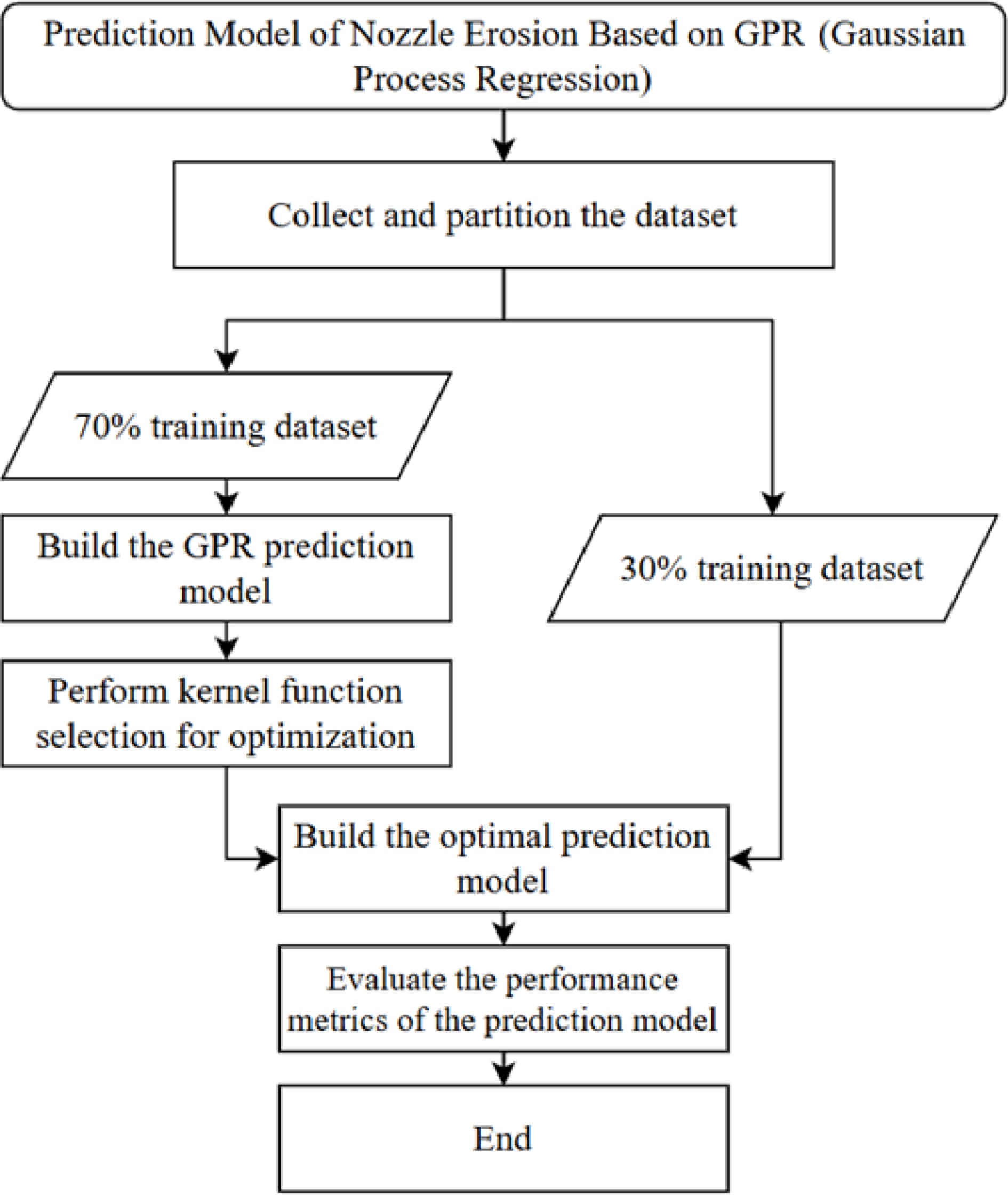
Figure 1.
Solution procedure of the prediction model.
-
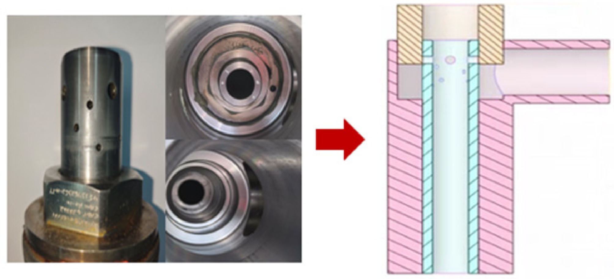
Figure 2.
Geometric model of the CV10 adjustable nozzle in Well HT101.
-
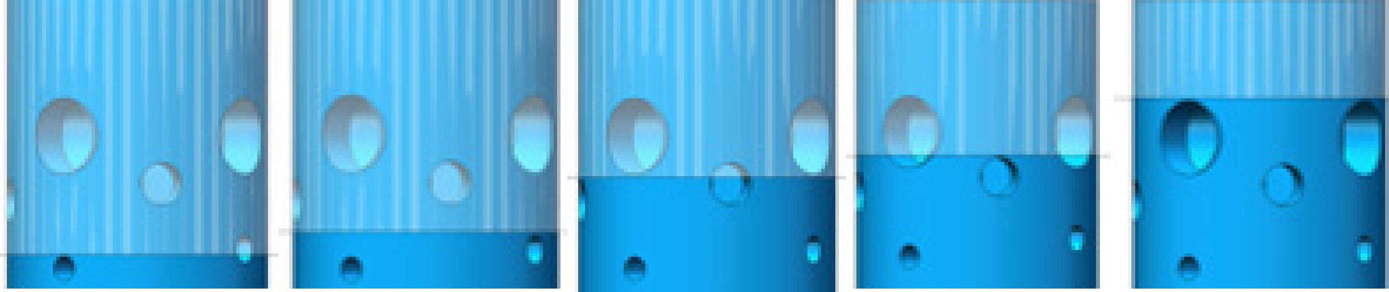
Figure 3.
Valve core of the CV10 adjustable nozzle under different opening conditions.
-
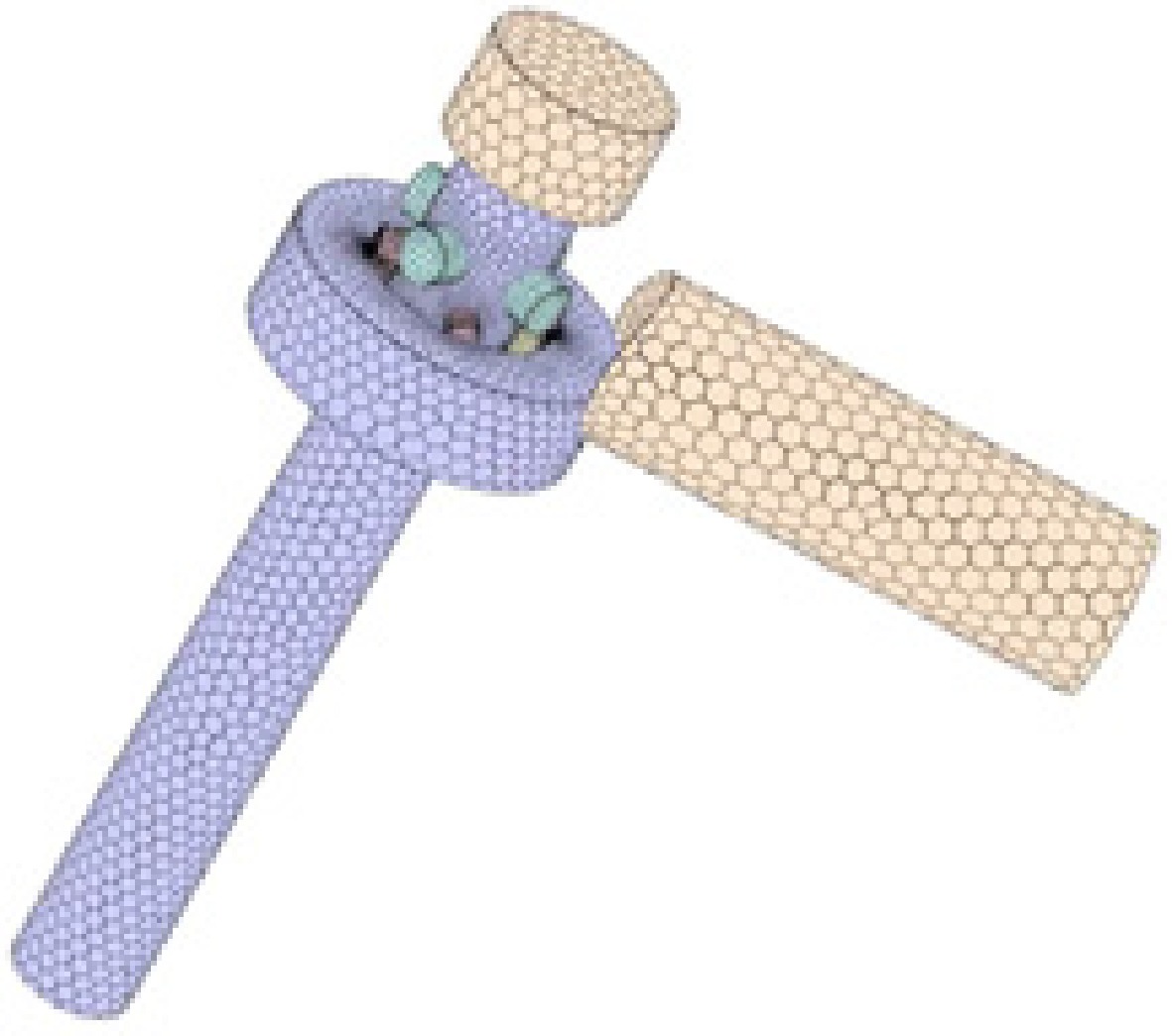
Figure 4.
Mesh generation of the CV10 adjustable nozzle model.
-
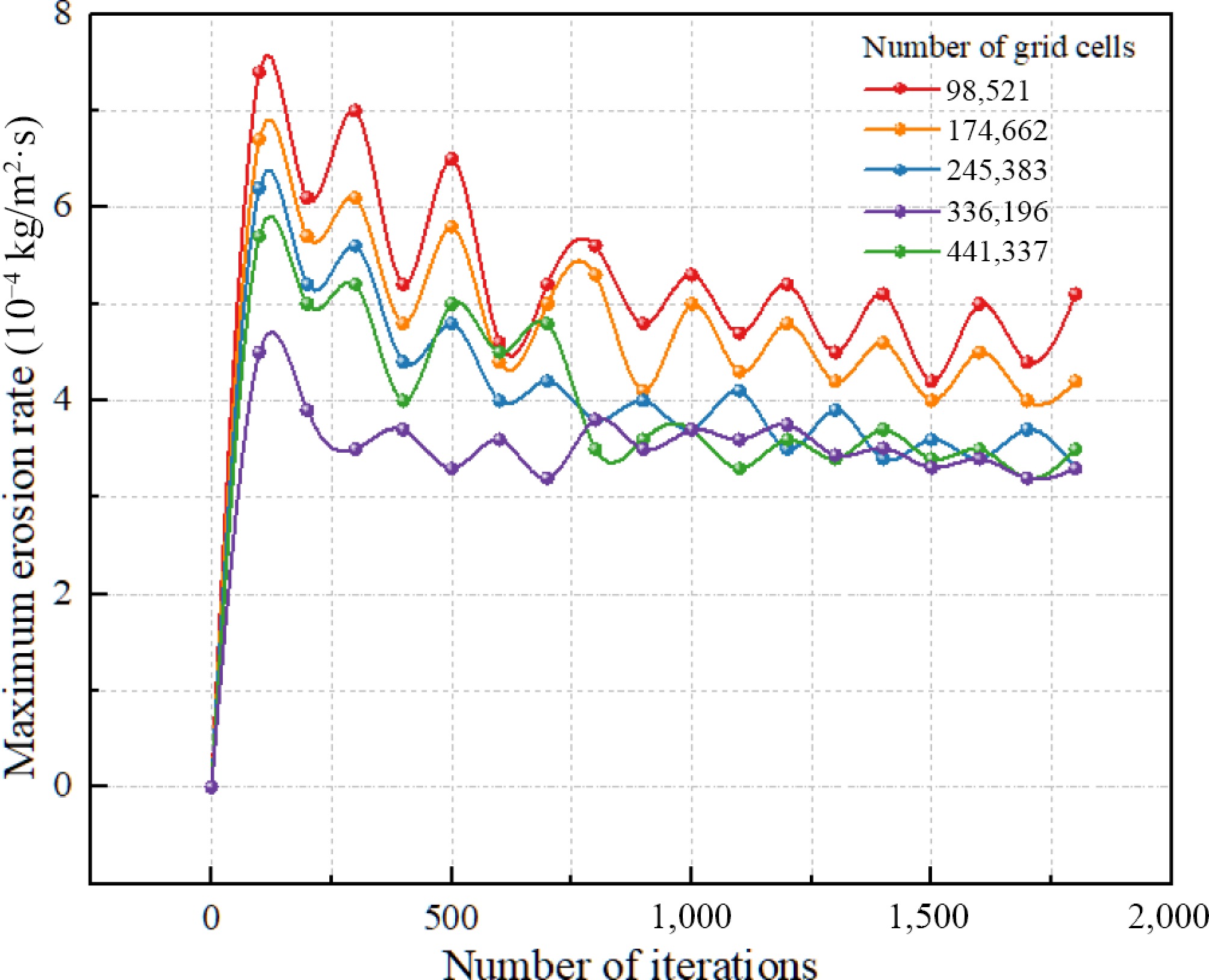
Figure 5.
Grid independence study.
-
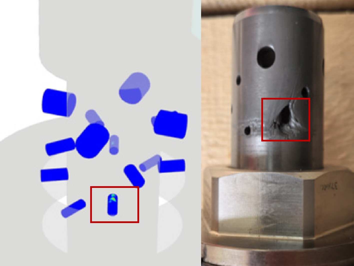
Figure 6.
Comparison of numerical simulation results with field observations.
-
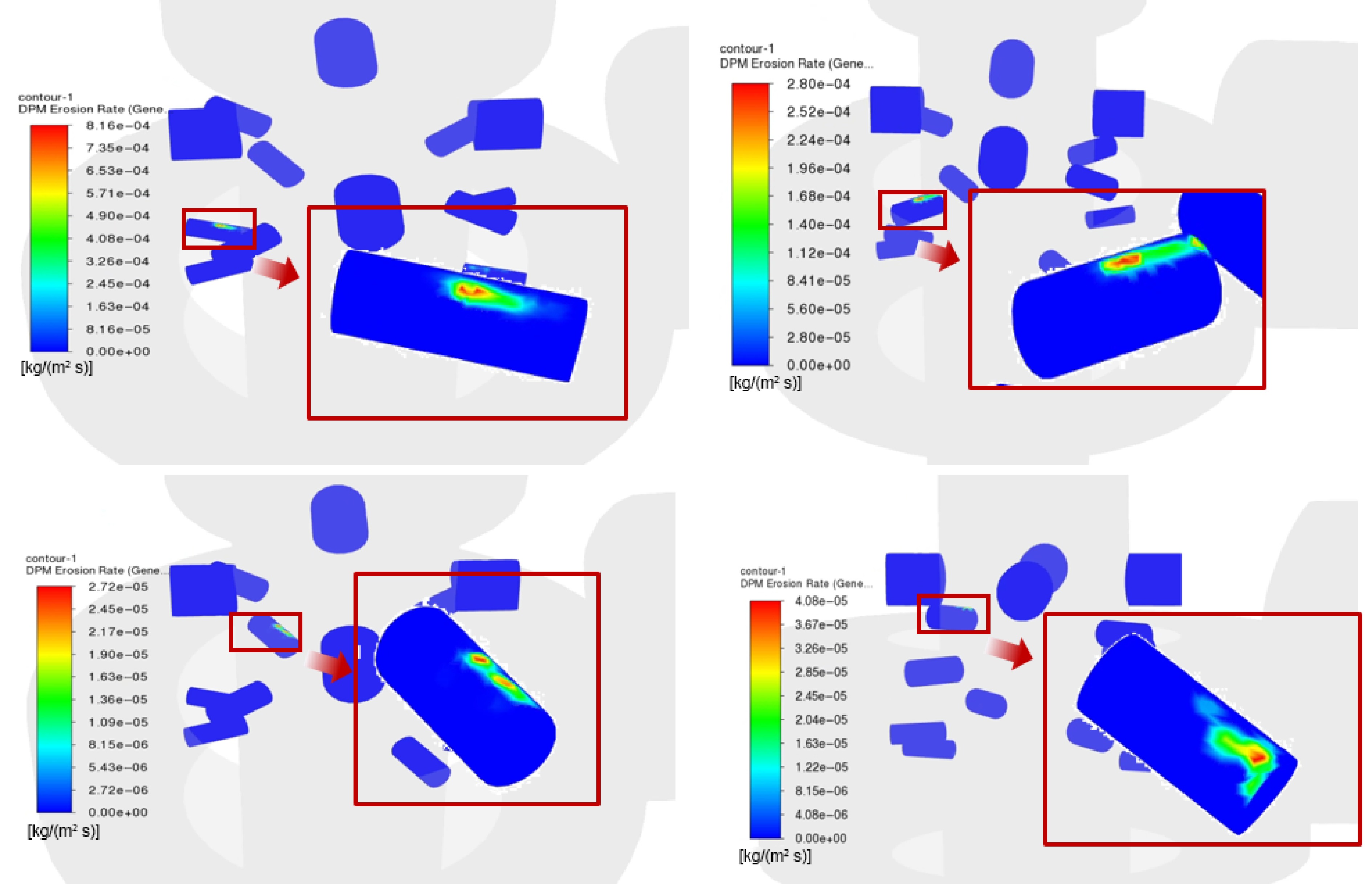
Figure 7.
Erosion rate contours of the adjustable nozzle under different opening conditions.
-
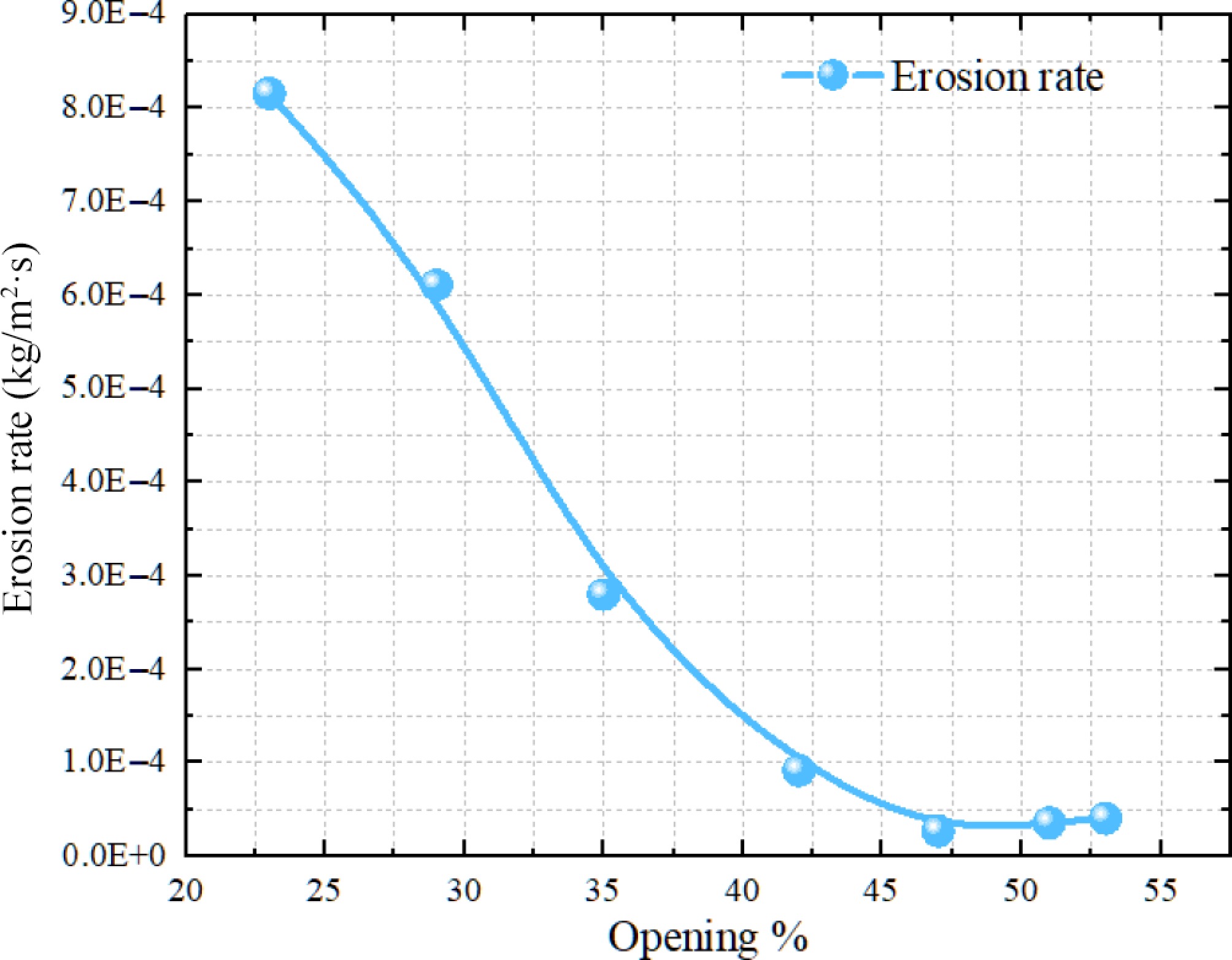
Figure 8.
Effect of nozzle opening on the erosion rate.
-
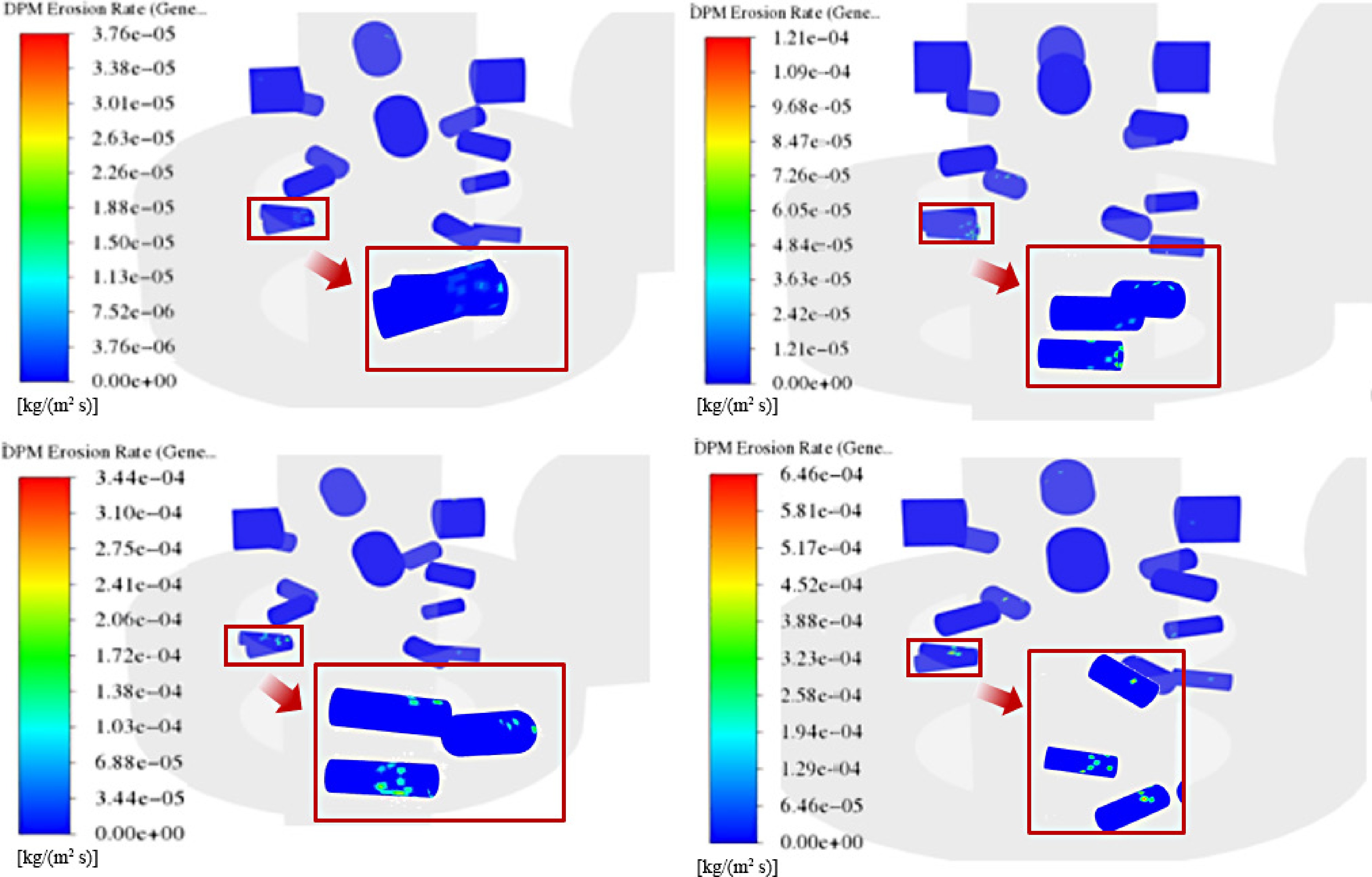
Figure 9.
Erosion rate contours under different production pressure differentials.
-
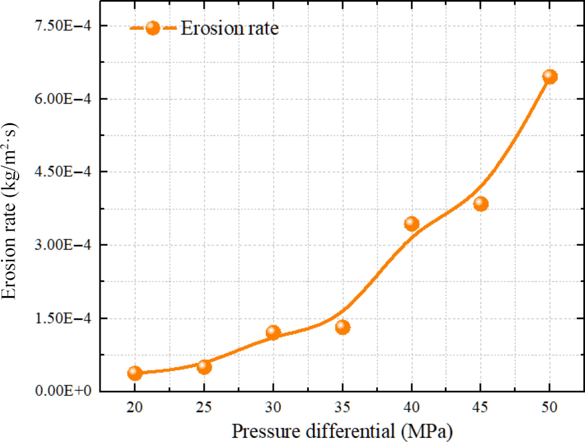
Figure 10.
Effect of production pressure differential on the erosion rate.
-
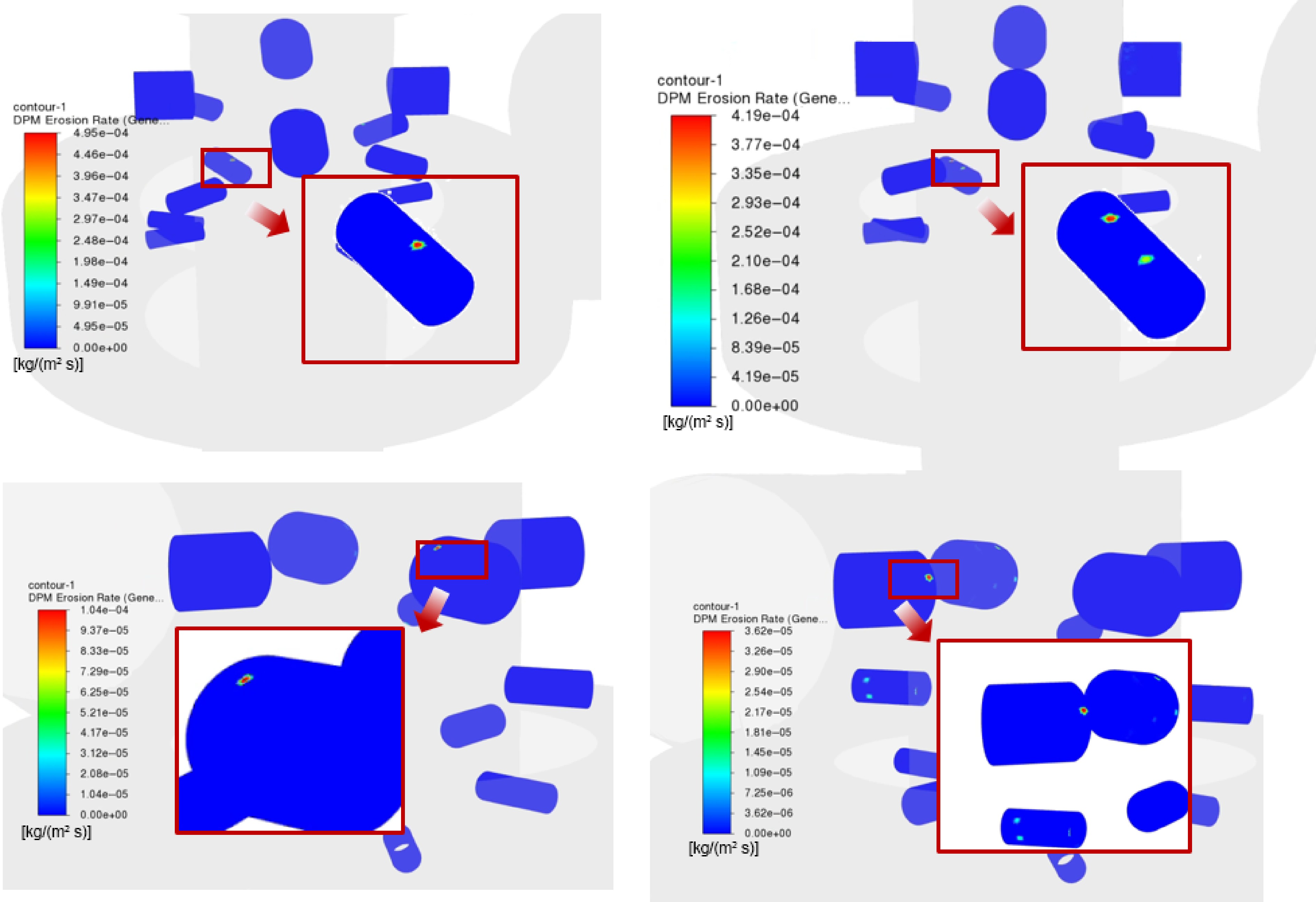
Figure 11.
Erosion rate contours of the adjustable nozzle under different particle diameters.
-
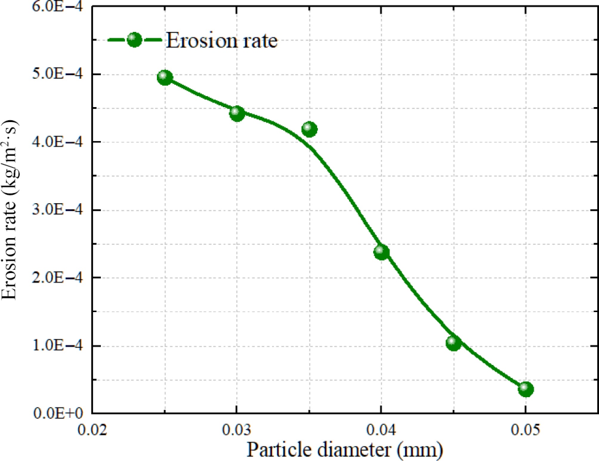
Figure 12.
Effect of particle diameter on the erosion rate.
-
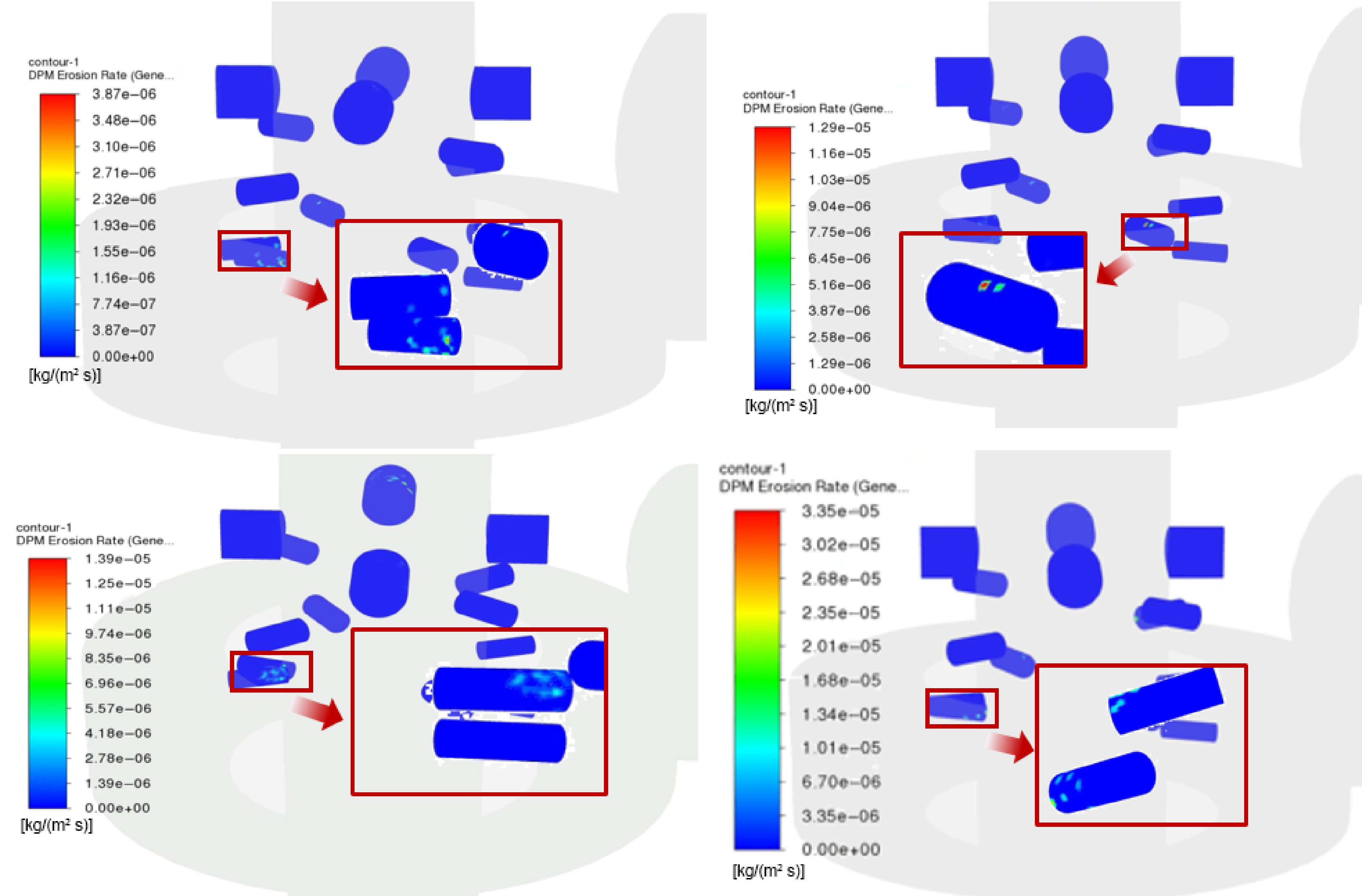
Figure 13.
Erosion rate contours of the adjustable nozzle under different particle densities.
-
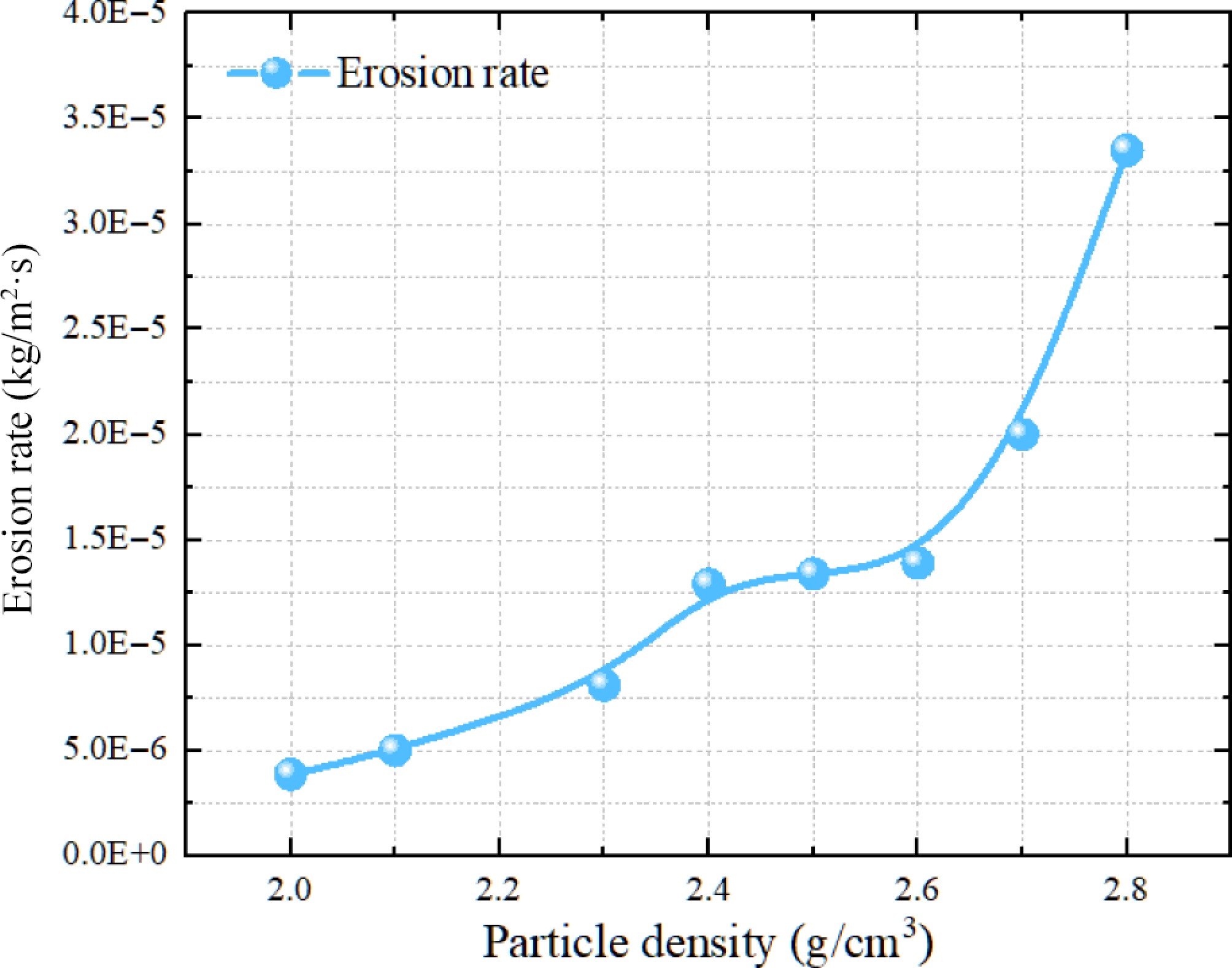
Figure 14.
Effect of particle density on the erosion rate.
-
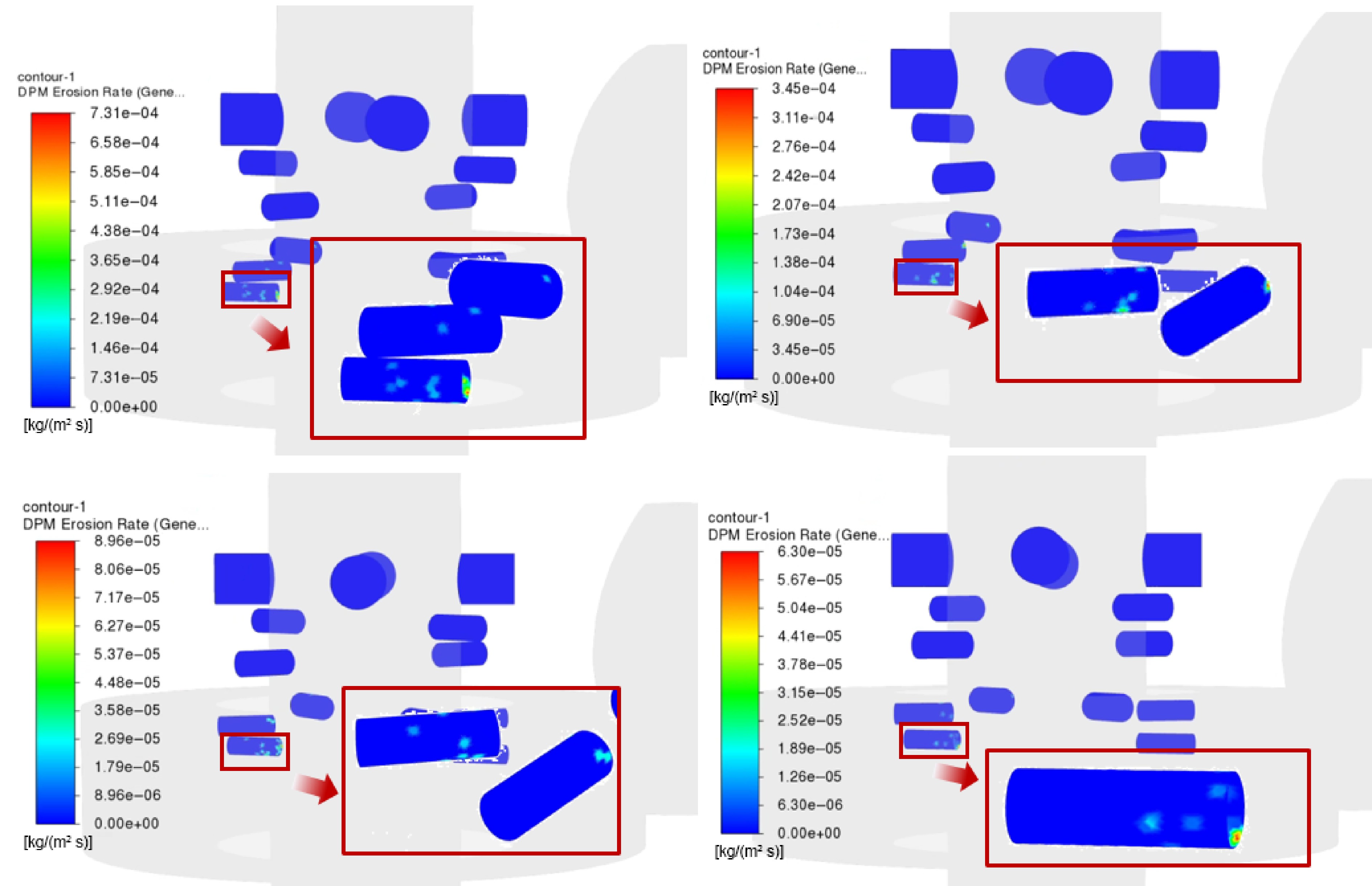
Figure 15.
Effect of sand production rate on the erosion rate.
-
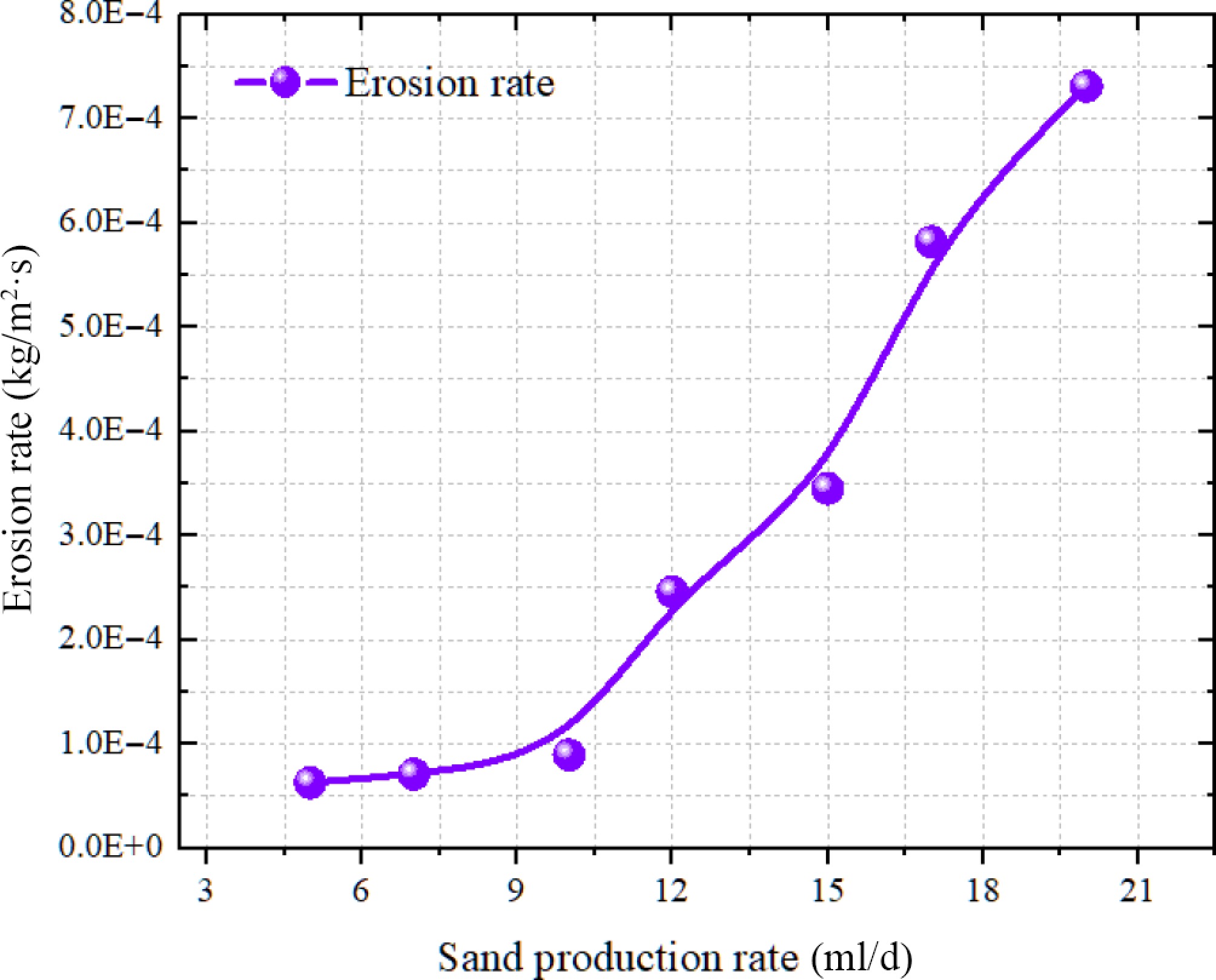
Figure 16.
Effect of sand production rate on the erosion rate.
-
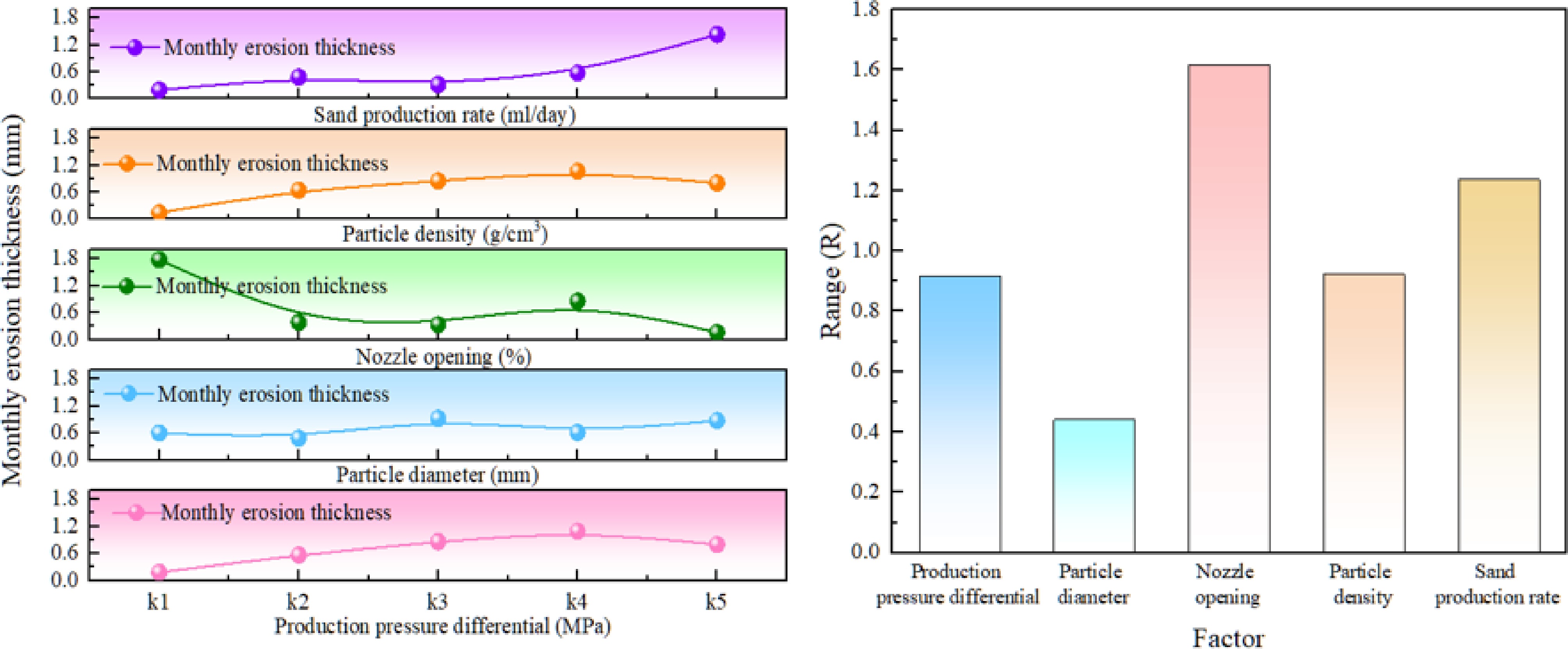
Figure 17.
Range analysis results.
-
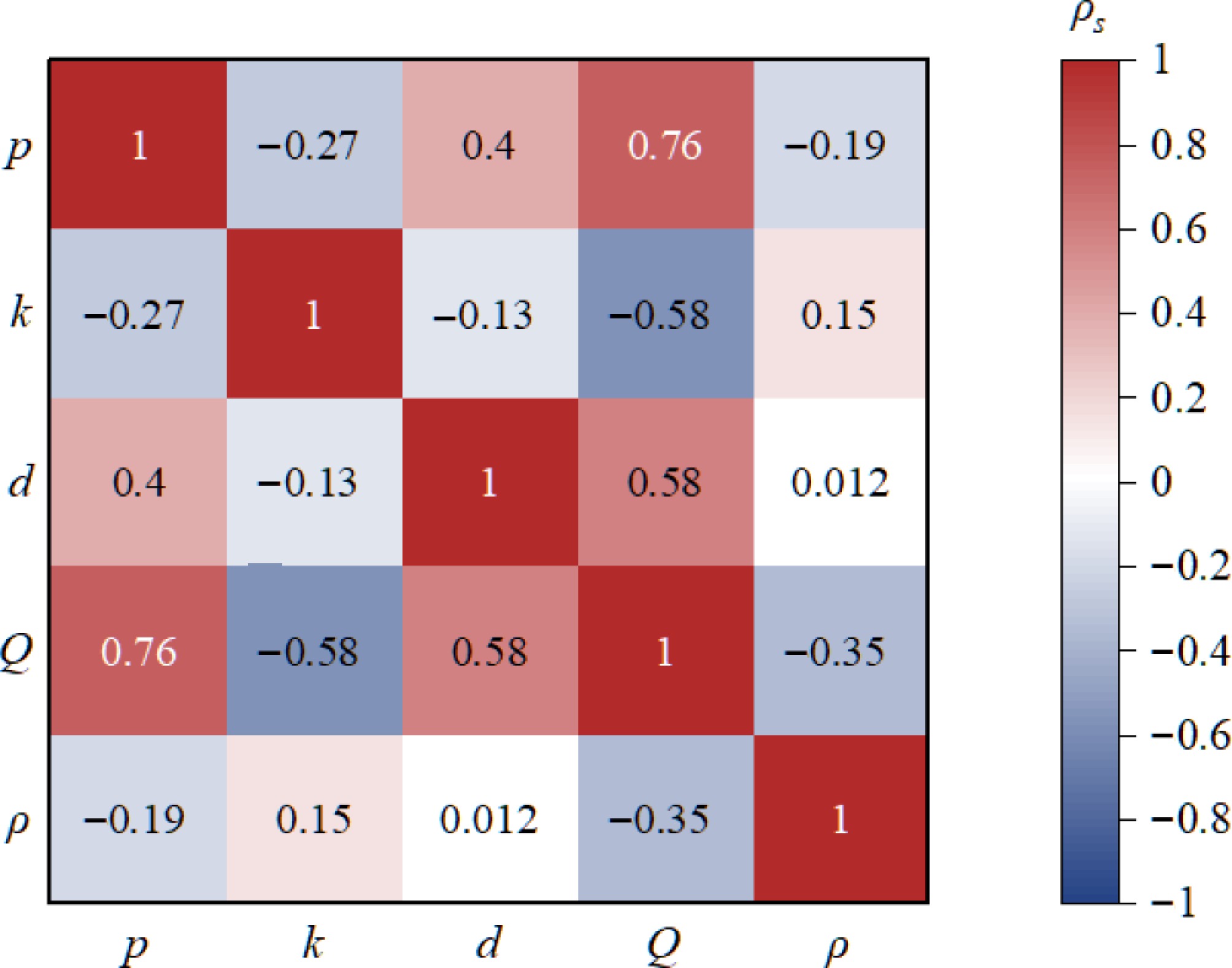
Figure 18.
Feature correlation analysis
-
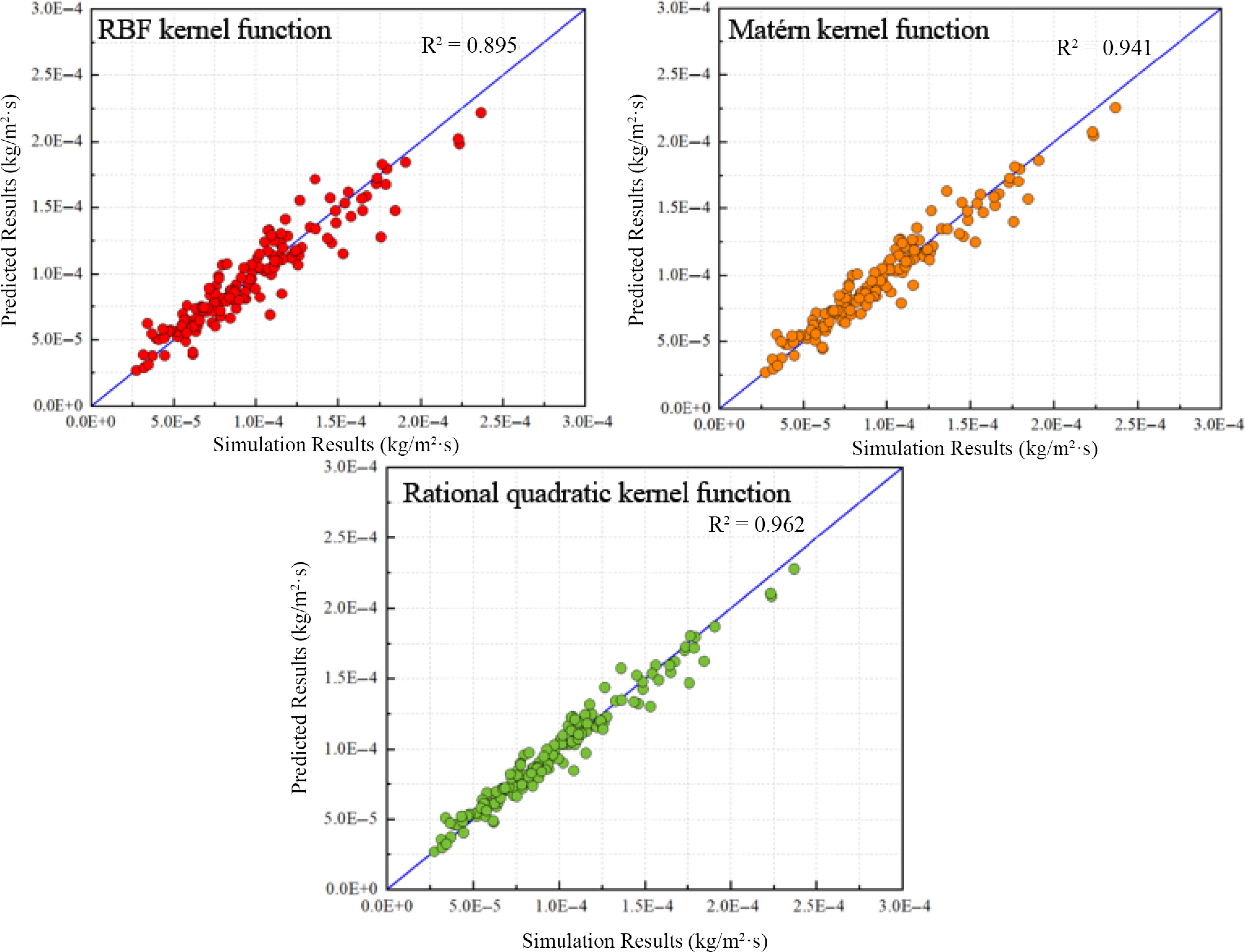
Figure 19.
Predicted erosion-rate results for the training set.
-
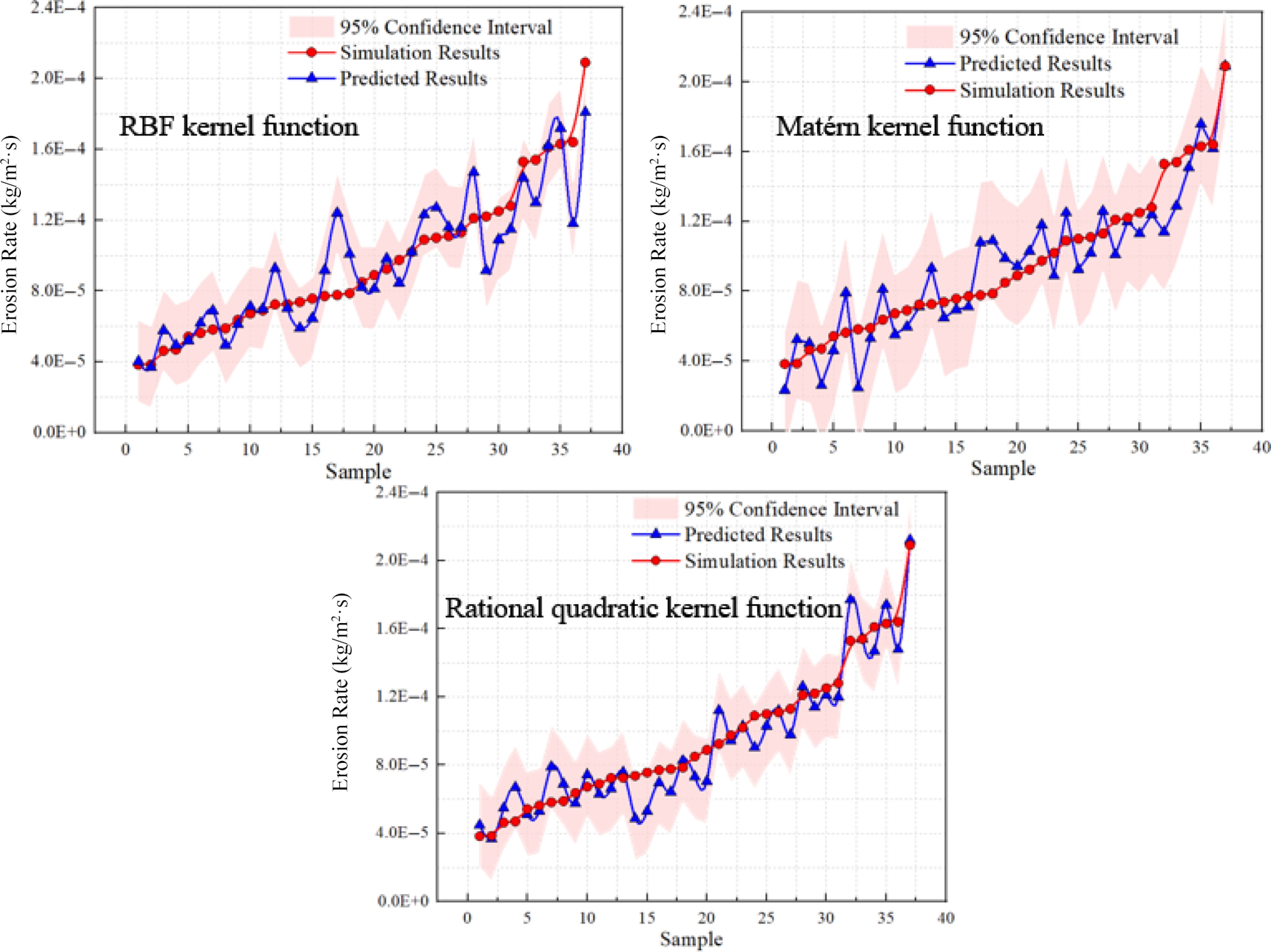
Figure 20.
Predicted erosion-rate results.
-
Numerical simulation parameter Value Inlet pressure of nozzle, p1/(MPa) 82 Outlet pressure of nozzle, p2/(MPa) 10 Particle mass flow rate, m1/(kg/s) 0.002 Particle density, ρ1/(kg/m3) 2,500 Particle diameter, d1/(μm) 25 Table 1.
Parameters used for the grid independence study.
-
Factor level Nozzle opening (%) Production pressure differential (MPa) Particle diameter (μm) Particle density (g/cm3) Sand production rate (ml/d) 1 23 20 25 2 5 2 29 25 30 2.2 10 3 35 30 35 2.4 15 4 47 35 40 2.6 20 5 53 40 45 2.8 25 Table 2.
Factor levels for the orthogonal experimental design.
-
Run No. Nozzle opening (%) Production pressure differential (MPa) Particle diameter (μm) Particle density (g/cm3) Sand Production rate (ml/d) Erosion thickness (mm) 1 23 20 25 2 5 0.044 2 29 20 30 2.2 10 0.22 3 35 20 35 2.4 15 0.005 4 47 20 40 2.6 20 0.63 5 53 20 45 2.8 25 0.02 6 29 25 25 2.4 15 0.31 7 35 25 30 2.6 20 0.018 8 47 25 35 2.8 25 0.55 9 53 25 40 2 5 0.21 10 23 25 45 2.2 10 1.73 11 35 30 25 2.8 25 1.49 12 47 30 30 2.2 5 0.21 13 53 30 35 2.4 10 0.08 14 23 30 40 2.6 15 1.74 15 29 30 45 2.8 20 0.8 16 47 35 25 2.4 10 1.03 17 53 35 30 2.6 15 0.36 18 23 35 35 2.8 20 3.75 19 29 35 40 2 25 0.33 20 35 35 45 2.2 5 0.002 21 53 40 25 2.6 20 0.13 22 23 40 30 2.8 25 1.62 23 29 40 35 2.2 5 0.25 24 35 40 40 2.4 10 0.15 25 47 40 45 2.8 15 1.84 Table 3.
Experimental scheme and results of the orthogonal design.
-
k value Production pressure differential Particle diameter Nozzle opening Particle density Sand production rate k1 0.1838 0.6008 1.7768 0.1432 0.194 k2 0.5636 0.4856 0.382 0.642 0.4824 k3 0.864 0.927 0.333 0.851 0.315 k4 1.0944 0.612 0.852 1.0656 0.5756 k5 0.798 0.8784 0.16 0.802 1.43 R 0.9156 0.4414 1.6168 0.9224 1.236 Table 4.
Results of the range analysis.
-
Kernel function Nozzle erosion rate R2 RMSE/(kg/m2·s) MSE/(kg2/m4·s2) RBF 0.835 1.71 × 10⁻⁵ 2.92 × 10⁻¹⁰ Matérn 0.829 1.67 × 10⁻⁵ 2.78 × 10⁻¹⁰ Rational quadratic 0.910 1.21 × 10⁻⁵ 1.47 × 10⁻¹⁰ Table 5.
Performance evaluation of GPR models with different kernel functions.
Figures
(20)
Tables
(5)