Study on the erosion characteristics and predictive modeling of surface throttling in ultra-high-pressure gas condensate wells

The southern margin block of the Xinjiang Oilfield is located in the southern Junggar Basin. This region has undergone intense tectonic compression, resulting in complex geological structures and widespread overpressure within the strata^[1,2]. Under conditions of large production pressure differentials, the stress state of the reservoir rock in the completed interval becomes highly complex. The interaction of multiple factors readily induces reservoir damage and sand production^[3], thereby affecting the production stability of gas wells. As sand-laden gas flows enter the surface gathering and transportation system, solid particles continuously impinge upon surface facilities. In particular, the choke nozzle is highly susceptible to severe erosion under the combined effects of high-velocity gas flow and particle impingement. Taking Well HT101 in the Xinjiang Oilfield as an example, analysis of solid particles collected from the desander indicates that their lithological characteristics are essentially consistent with those of the reservoir sand. After the sand-laden gas enters the surface manifold and throttling device, the erosion of the choke nozzle is further aggravated. Therefore, investigating the erosion characteristics and developing predictive models for surface choke nozzles in ultra-high-pressure gas condensate wells is of significant practical importance. Systematically elucidating the sources and evolution mechanisms of nozzle erosion and establishing corresponding predictive models can provide a theoretical basis for equipment optimization and operational management. This, in turn, will help extend equipment service life, reduce failure rates, and enhance the safety and economic performance of oil and gas field production^[4]. The related research outcomes can also offer scientific support for equipment management, maintenance strategies, and production safety assurance in ultra-high-pressure gas wells, thereby promoting the efficient and safe development of oil and gas resources.

Numerous scholars have conducted substantial and productive research on the analysis and prediction of erosion in surface throttling systems of gas wells. With respect to erosion wear mechanisms, Zhang et al.^[5] developed a three-dimensional CFD model to evaluate erosion in natural gas choke valves with different structures. Guo et al.^[6] used CFD to analyze erosion in high-temperature, high-pressure choke valves. Li et al.^[7] reviewed erosion models and identified key factors and mechanisms governing valve erosion. Zhao et al.^[8] applied a CFD–DPM model to investigate needle valve erosion under shale gas operating conditions. Wu et al.^[9] established a CFD–DEM-based gas–solid erosion model for needle-type valves. Liu et al.^[10] examined cage valve erosion under gas–liquid–solid three-phase flow, focusing on internal flow passages. Jing et al.^[11] investigated erosion-induced failure of side valve plates through liquid–solid experiments and simulations. Sun et al.^[12] applied CFD–DEM to study erosion in small-diameter butterfly valves under gas–solid flow. Kou et al.^[13] numerically examined erosion in sleeve-type discharge valves during operation. Zhao et al.^[14] combined CFD with the FINNIE model to analyze valve-core erosion and proposed an optimized orifice structure to mitigate wear. Existing studies on erosion wear have mainly focused on low-pressure conditions and simplified structures, often neglecting the coupled effects of pressure, particle properties, geometry, and material. In contrast, erosion behavior under ultra-high-pressure conditions remains insufficiently explored. This is particularly true for electrically adjustable nozzles with complex flow passages and dynamic regulation, where erosion exhibits stronger nonlinearity and localized concentration. Overall, systematic investigations targeting ultra-high-pressure and structurally complex nozzles are still lacking.

Meanwhile, numerous studies have been conducted on predictive models for erosion in throttling nozzles. Wang et al.^[15] developed a machine learning-based model to predict erosion in natural gas pipeline elbows. Liu et al.^[16] combined CFD with machine learning methods, including LSTM and BP neural networks, to predict erosion rates under different operating conditions. Another study by Wang et al.^[17] integrated machine learning with multi-objective optimization to establish a data-driven erosion rate model. Li et al.^[18] coupled CFD and the Euler–Lagrange approach with machine learning to predict erosion in tandem elbows under gas–solid flow. Wang et al.^[19] applied a genetic algorithm–optimized extreme learning machine (GA-ELM) to forecast elbow erosion. Chen et al.^[20] used a kernel extreme learning machine (KELM) to model the relationship between key features and erosion rate. Peng et al.^[21] combined the sparrow search algorithm with support vector machines to develop an erosion prediction model. Brown et al.^[22] reviewed common erosion prediction methods and highlighted limitations of machine learning approaches, particularly regarding data sparsity and feature correlation. However, most existing erosion prediction models rely on large-scale datasets and are typically developed using deep machine learning techniques. For surface throttling conditions in ultra-high-pressure gas condensate wells, systematic experimental investigations are constrained by safety concerns, technical limitations, and high costs. Consequently, current research primarily depends on numerical simulations, resulting in limited sample sizes, restricted data distributions, and considerable uncertainty. Under such conditions, conventional machine learning methods often struggle to establish stable and reliable predictive models. Therefore, it is necessary to introduce learning strategies tailored for small-sample scenarios to enable robust prediction of erosion wear in ultra-high-pressure gas condensate well surface throttling systems.

Accordingly, this study focuses on two core aspects: First, the erosion–wear characteristics of surface throttling at the wellhead of ultra-high-pressure gas condensate wells; second, the development of an erosion rate prediction model under small-sample conditions. Based on CFD simulations, the coupled dynamics between high-velocity gas flow and particle motion in ultra-high-pressure gas–solid two-phase flow are systematically investigated. Particular attention is given to revealing the spatial distribution and evolution of erosion in complex electrically adjustable nozzles under multi-factor coupling, thereby highlighting the unique mechanisms and increased complexity of erosion under ultra-high-pressure operating conditions. On this basis, Gaussian Process Regression (GPR) is introduced to develop a small-sample surrogate model for erosion prediction in complex engineering systems. Benefiting from its nonparametric Bayesian framework, the method exhibits strong knowledge generalization capability under limited data conditions. At the same time, it enables rapid representation and prediction of complex erosion processes through an efficient surrogate modeling strategy. In addition, the inherent uncertainty quantification capability of the GPR model provides confidence information for the predictions, thereby offering valuable support for risk assessment and decision-making in engineering applications. In summary, from an integrated perspective combining mechanism analysis and data-driven modeling, this study innovatively elucidates the erosion–wear characteristics of ultra-high-pressure throttling processes and proposes a reliable prediction approach suitable for small-sample scenarios, providing both theoretical insights and engineering guidance for equipment life assessment and structural optimization.

CFD-based erosion modeling generally involves two main steps: (1) The flow field of the continuous phase is modeled by considering the gas as a continuum, with its motion governed by the Navier–Stokes equations; and (2) particle tracking and erosion calculation, where particles are considered as the discrete phase and their motion is governed by Newton's second law.

2.1.1.   Governing equations of fluid flow

The general forms of the continuity equation and the momentum conservation equation are given in Eqs. (1) and (2), respectively^[23,24]:

In Eqs. (1) and (2), ρ_g denotes the density of the continuous phase, kg/m³; u represents the velocity vector of the continuous phase, m/s; p is the pressure, Pa; g is the gravitational acceleration, m/s²; and S_M denotes the interaction force between the discrete and continuous phases. τ is the stress tensor, which is expressed as Eq. (3):

where, µ denotes the dynamic viscosity of the fluid, Pa·s, and I represents the identity tensor.

The energy conservation equation is given as Eq. (4)^[25]:

where, E denotes the total energy per unit mass, J/kg; k is the thermal conductivity; T represents the fluid temperature, K; and q is the heat source term associated with the erosion process.

2.1.2.   Turbulence model

The internal structure of the adjustable nozzle is geometrically complex, leading to velocity gradients, flow separation, and vortex formation within the flow field. To capture turbulence characteristics, the RNG k–ε model is utilized owing to its enhanced accuracy and broader applicability. The governing equations are given in Eqs. (5) and (6)^[26]:

In Eqs. (5) and (6), µ_eff denotes the effective viscosity, Pa·s; G_k and G_β represent the production terms of turbulent kinetic energy, Pa/s; α_k and α_e are the inverse effective Prandtl numbers for k and ε, respectively (dimensionless), typically taken as 1.39; ε is the turbulent dissipation rate, m²/s³; k is the turbulent kinetic energy, m²/s²; C₁ε and C₂ε are empirical constants (dimensionless); x_j denotes the second component of the position vector (dimensionless); µ_t is the turbulent viscosity, Pa·s; and R_ε is an additional source term, Pa/s².

2.1.3.   Governing equation for discrete phase motion

In the numerical simulation, eroding particles are treated as the discrete phase and solved using the Discrete Phase Model (DPM). The governing equations of particle motion are given in Eqs. (7)–(9)^[27]:

Where,

In Eqs. (7)–(9) f_D denotes the drag function; C_D represents the drag coefficient; u_p is the particle-phase velocity, m/s; dp is the particle diameter, m; ρ_p is the particle density, kg/m³; u is the fluid-phase velocity, m/s; µ is the dynamic viscosity of the fluid phase, Pa·s; ρ is the fluid density, kg/m³; Re denotes the Reynolds number (dimensionless); and F_s represents other forces acting on the particles, N.

2.1.4.   Particle–wall collision model

To accurately predict particle trajectories, it is essential to employ an appropriate particle–wall collision model. The variation in particle velocity upon impact with the wall is typically characterized by the restitution coefficient. In the present study, the particle–wall collision model proposed by Cui et al. and Cui et al.^[28,29] was adopted to improve the accuracy of particle dynamics simulation. The governing equations of the particle–wall collision model are given in Eqs. (10) and (11)^[28,29].

In Eqs. (10) and (11), e_n and e_t denote the normal and tangential restitution coefficients, respectively, while α represents the particle impingement angle on the wall surface.

2.1.5.   Erosion model

The erosion rate of the adjustable nozzle is characterized as the material mass loss per unit time resulting from particle impingement, and is evaluated using the model described in Eq. (12)^[30].

In this equation, R_E denotes the erosion rate, kg/(m²·s); A_face represents the wall surface area, m²; m_i is the particle mass flow rate, kg/s; v is the particle impact velocity, m/s; b(v) denotes the velocity exponent function; C(d_i) represents the particle size function, which is taken as 1.8 × 10⁻⁹ in the present study; and f(α) is the particle impingement angle function, defined using a piecewise linear formulation.

2.2.   Nozzle erosion rate prediction model

Gaussian Process Regression (GPR) is a non-parametric approach to regression grounded in Bayesian principles and statistical learning theory, designed to model the joint probability distribution of a finite collection of random variables. In addition, GPR provides both predictive mean values and corresponding uncertainty estimates, enabling probabilistic quantification of nozzle erosion risk. This capability enhances the reliability of model predictions and strengthens its support for engineering decision-making. Therefore, GPR demonstrates considerable potential for applications in nozzle service life prediction and operational optimization.

2.2.1.   Gaussian process regression

Gaussian Process Regression (GPR) is a non-parametric regression method developed based on Bayesian theory and statistical learning theory, aiming to establish the joint probability distribution over a finite set of random variables. In addition to providing point predictions, GPR is capable of quantifying predictive uncertainty in the form of confidence intervals, which can be expressed as follows^[31,32]:

In Eqs. (13)–(15), µ(X) denotes the mean function of the Gaussian process, which is commonly assumed to be zero, and k(X,X′) represents the kernel (covariance) function.

Assume that the training dataset is given by {(X_i,y_i)|i=1,2,3,…,n}. The relationship between the input features and the output can be expressed as follows:

In this equation, y_i denotes the observed value with noise; f(X_i) represents the latent function value corresponding to the input vector X_i; and ε is the Gaussian noise term, assumed to follow a normal distribution ε~N(0, σ²).

When constructing a model using GPR, the mean function is typically assumed to be µ(X) = 0, and an appropriate kernel function parameterized by θ is selected. The hyperparameters θ generally include a set of control parameters, which are determined by minimizing the negative log-likelihood (NLL). The NLL can be expressed as follows^[33]:

In this equation, X = [X₁,X₂,X₃,…,X_n] denotes the matrix of input variables, and Y = [Y₁,Y₂,Y₃,…,Y_n]^T represents the corresponding output vector.

After selecting an appropriate kernel function and given the training data, the joint distribution of the training outputs and the test outputs follows a Gaussian distribution. According to Bayesian inference, the predictive distribution of the output y* corresponding to a new input X*, i.e., P(y*|X*, θ), can be derived as follows^[34]:

In Eqs. (18), (19), µ* and Σ* denote the predictive mean and variance, respectively, which are used to perform point prediction and construct confidence intervals for the test output y*.

2.2.2.   Kernel function selection

In Gaussian Process Regression (GPR), the covariance function (kernel) plays a central role, as it defines the prior and posterior distributions by measuring the similarity between data points. Different kernels lead to different model structures and probabilistic behaviors. In this study, three commonly used kernels—the Radial Basis Function (RBF), Matérn, and Rational Quadratic—were employed to construct GPR models, and their performance in erosion rate prediction was comparatively evaluated.

(1) RBF Kernel. The Radial Basis Function (RBF) kernel, also known as the squared exponential kernel, is parameterized by a length-scale parameter l (l > 0). The length scale l can be either a scalar or a vector with the same dimensionality as the input variable x. A larger value of l corresponds to a smoother function and smaller variance between training points. The mathematical form of the RBF kernel is given as follows^[35]:

In this equation, d(x_i,x_j) denotes the Euclidean distance between x_i and x_j.

(2) Matérn Kernel. The Matérn kernel is an extension of the RBF kernel. It is parameterized by a length-scale parameter l (l > 0) and introduces an additional smoothness parameter v, which controls the differentiability and smoothness of the function. The Matérn kernel is defined as follows^[36]:

In this equation, K_v denotes the modified Bessel function of the second kind, and Г(v) represents the Gamma function evaluated at v. The smoothness parameter v is commonly set to 0.5, 1.5, or 2.5. Smaller values of v correspond to less smooth function realizations.

(3) Rational Quadratic Kernel. The Rational Quadratic kernel serves as an alternative to the RBF kernel and can be interpreted as a weighted sum of RBF kernels with different characteristic length scales. It is parameterized by a length-scale parameter l (l > 0) and a scale-mixture parameter α (α > 0), where α controls the relative weighting of different length scales. Although the Rational Quadratic kernel has a wide range of applicability, it is relatively sensitive to hyperparameter settings. The mathematical expression of this kernel is given as follows^[37]:

In this equation, α represents the relative weighting of different characteristic length scales.

2.2.3.   Prediction model solution procedure

The overall framework of the Gaussian Process Regression (GPR)-based erosion prediction model for surface throttling in ultra-high-pressure condensate gas wells is illustrated in Fig. 1 The specific procedure is described as follows:

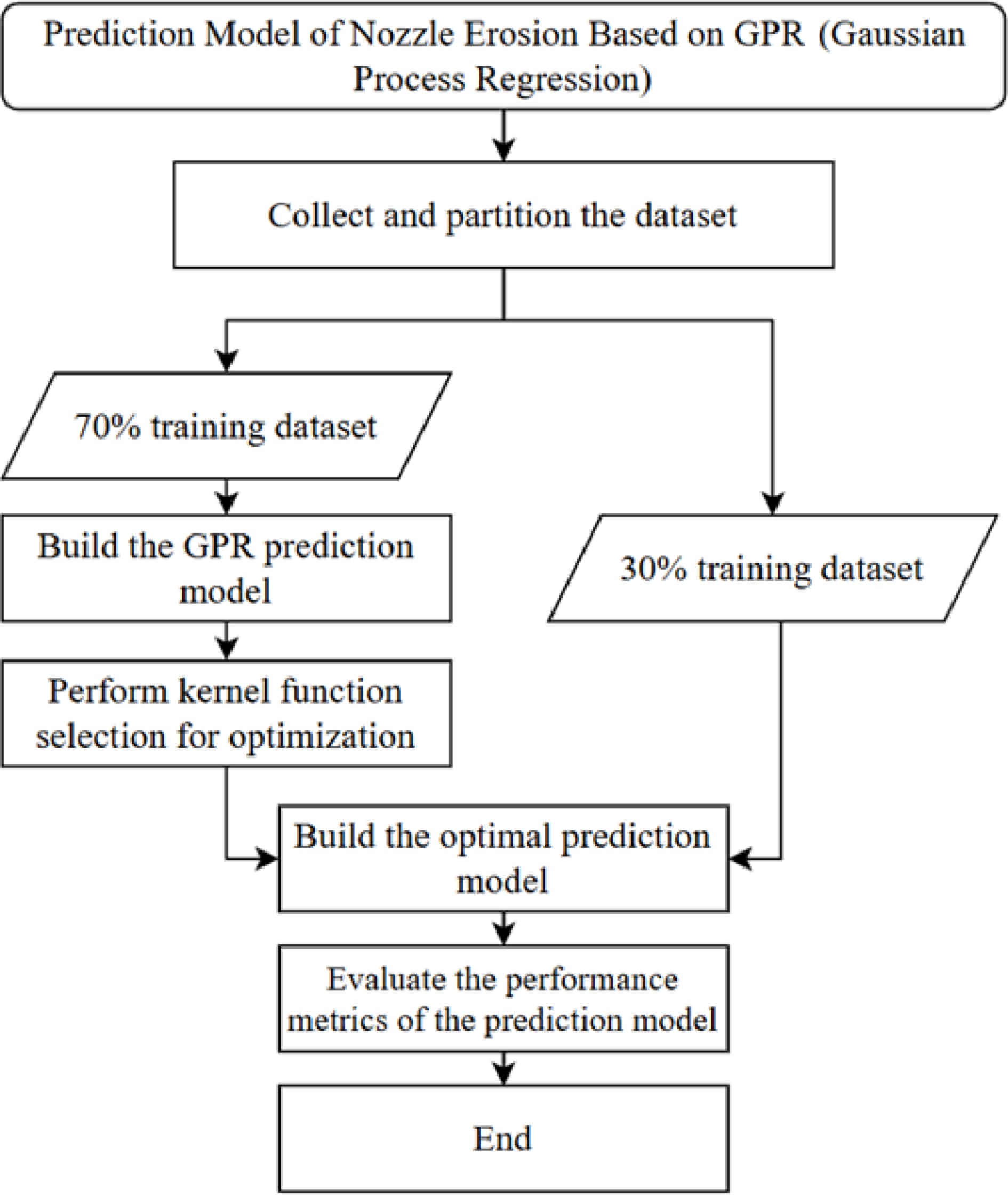
Figure 1. 

Solution procedure of the prediction model.

(1) Based on the hourly production data of Well HT101, key parameters such as pressure differential, particle density, and particle diameter were extracted as input variables, while the erosion rate was taken as the output;

(2) These parameters were then implemented in ANSYS Fluent to simulate and obtain the corresponding erosion rates;

(3) The dataset was split into training and testing subsets, where the former was used for model development and the latter for performance evaluation;

(4) Kernel functions were selected according to the problem characteristics, and RBF, Matérn, and Rational Quadratic kernels were compared to identify the most suitable one for the Gaussian Process Regression model;

(5) The proposed model was further validated using the test data, and its predictive performance was assessed using metrics such as RMSE and the coefficient of determination (R²).

2.2.4.   Model performance evaluation metrics

To reasonably evaluate the performance of the nozzle throttling erosion rate prediction model, RMSE and the coefficient of determination (R²) were adopted as evaluation metrics to measure the model's generalization capability. RMSE is widely used to quantify prediction errors in regression analysis, reflecting the difference between predicted and actual values, and ranges from [0, +∞), with smaller values indicating better regression performance.

The coefficient of determination (R²) characterizes the proportion of variance in the target variable explained by the regression model, thereby reflecting the goodness of fit. R² takes values in the range (−∞, 1], with larger values indicating better fitting performance. The corresponding expressions are given as follows^[33]:

In Eqs. (24) and (25), n denotes the total number of samples; tᵢ and pᵢ represent the i observed value and predicted value, respectively; and t̄_i denotes the mean of the observed values.

Based on the measurement data of the critical components of the CV10 adjustable nozzle in Well HT101, a three-dimensional geometric model was developed using SolidWorks. The model incorporates key components, including the valve core, valve seat, and valve sleeve. It accurately represents the dimensions, geometries, and relative positions of these components, thereby providing a reliable geometric foundation for subsequent CFD simulations. The geometric model is shown in Fig. 2.

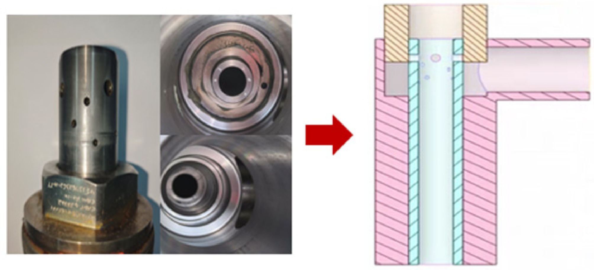
Figure 2. 

Geometric model of the CV10 adjustable nozzle in Well HT101.

To improve the accuracy of the simulation results, the model assembly was configured to match the actual assembly conditions. The CV10 adjustable nozzle was analyzed under different valve openings, as illustrated in Fig. 3. By adjusting the valve opening, the assembly configurations between the valve core and the valve seat were established for various opening conditions.

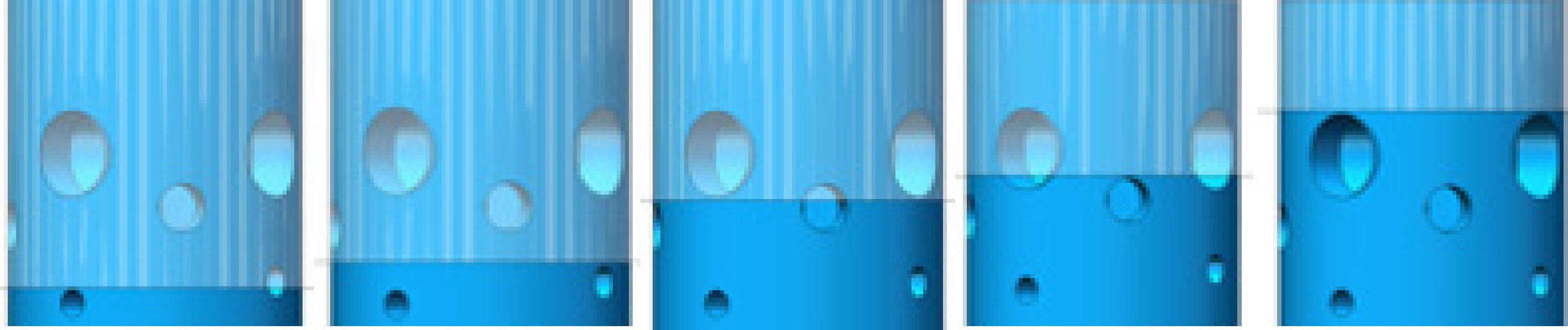
Figure 3. 

Valve core of the CV10 adjustable nozzle under different opening conditions.

The established CV10 adjustable nozzle model was discretized using a structured hexahedral mesh. Boundary layer refinement was applied to the inner wall of the nozzle to enhance near-wall resolution. During the meshing process, local mesh refinement was performed in critical regions of the model to accurately capture flow field variations and key features, as shown in Fig. 4. A well-designed mesh distribution contributes significantly to the accuracy and reliability of subsequent numerical simulations.

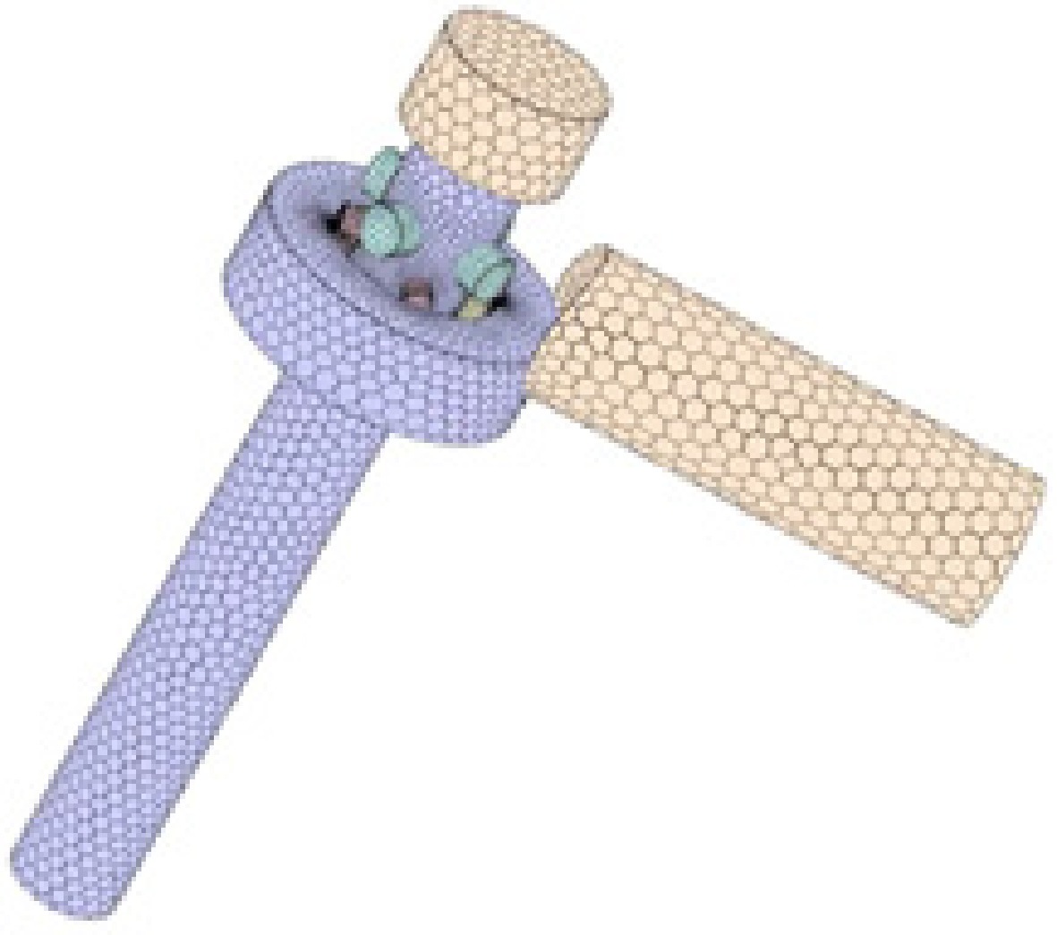
Figure 4. 

Mesh generation of the CV10 adjustable nozzle model.

To ensure computational accuracy while improving computational efficiency, a grid independence study was conducted. Five nozzle models with different mesh densities were generated, and erosion simulations were performed using the parameters listed in Table 1.

As shown in Table 1, the pressure differential between the inlet and outlet was set to 72 MPa. Based on sand production statistics at the wellhead, the particle mass flow rate was specified as 0.002 kg/s, with a particle density of 2,500 kg/m³ and a particle diameter of 25 μm. Under these operating conditions, a grid independence study was conducted to ensure the stability and reliability of the simulation results.

As shown in Fig. 5, when the number of grid cells reached 240,000 or more, the influence of mesh density on the computational results became negligible, and the results remained stable. Convergence was achieved after 1,000 iterations. Considering both computational efficiency and accuracy, a mesh consisting of 336,000 grid cells was ultimately selected, and 1,000 iterations were performed in the subsequent simulations.

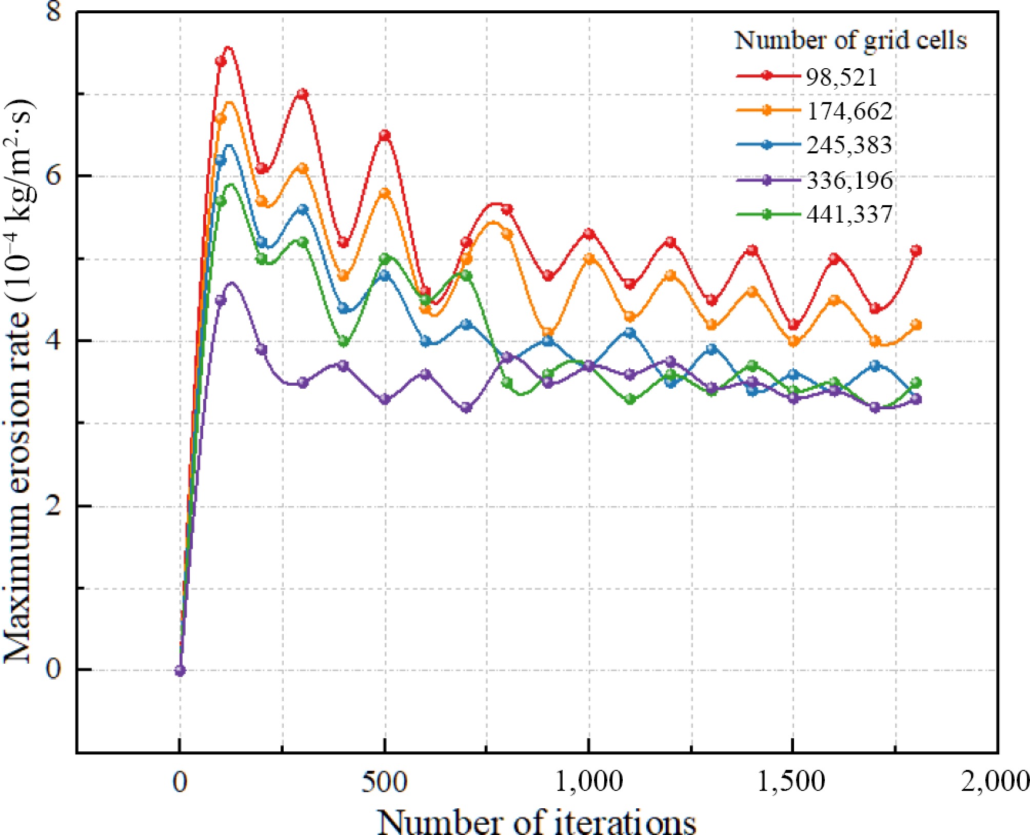
Figure 5. 

Grid independence study.

As presented in Fig. 6, the reliability and engineering applicability of the model are demonstrated; the numerical simulation results after grid independence verification were compared with field observations. The erosion locations were found to be consistent, mainly concentrated at the second row of valve holes on the backflow surface of the valve core, indicating that the numerical model exhibits good reliability.

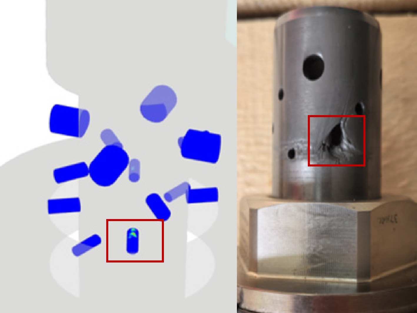
Figure 6. 

Comparison of numerical simulation results with field observations.

3.1.2.   Boundary conditions

According to the findings of Wang et al.^[38], the RNG k-ε model is better suited for simulating gas–solid two-phase flow in pipelines under the present conditions. In such flows, when the particle mass flow rate is significantly lower than that of the continuous phase, the effect of particles on the continuous phase can be considered negligible. Moreover, when the particle volume fraction is below 10%, the Discrete Phase Model (DPM) can be employed for numerical simulation.

Based on the above considerations, the RNG k-ε turbulence model combined with a CFD–DPM one-way coupling approach was adopted in this study. The RNG k-ε model effectively captures turbulence non-uniformity and anisotropy and is suitable for gas–solid interactions in complex flow fields. The CFD–DPM framework describes particles using a discrete phase model, enabling the simulation of particle trajectories and particle–wall interactions while coupling them with the continuous-phase flow.

To ensure computational accuracy and reliability, pressure inlet and pressure outlet boundary conditions were specified to accurately represent the inflow and outflow processes. To better account for gas compressibility, a density-based solver was employed to handle compressibility effects. In addition, the inner wall of the nozzle was defined as a no-slip boundary to properly model particle–wall interactions, thereby improving the overall accuracy and stability of the numerical simulations.

3.2.   Erosive wear characteristics of the nozzle

3.2.1.   Erosive wear of the adjustable nozzle at different openings

Based on the hourly production reports of Well HT101 and in conjunction with actual field operating conditions, the variation in erosion rate was investigated as the opening of the adjustable nozzle increased from 23.5% to 53%. The relationship between erosion rate and production pressure differential was obtained, as shown in Fig. 7.

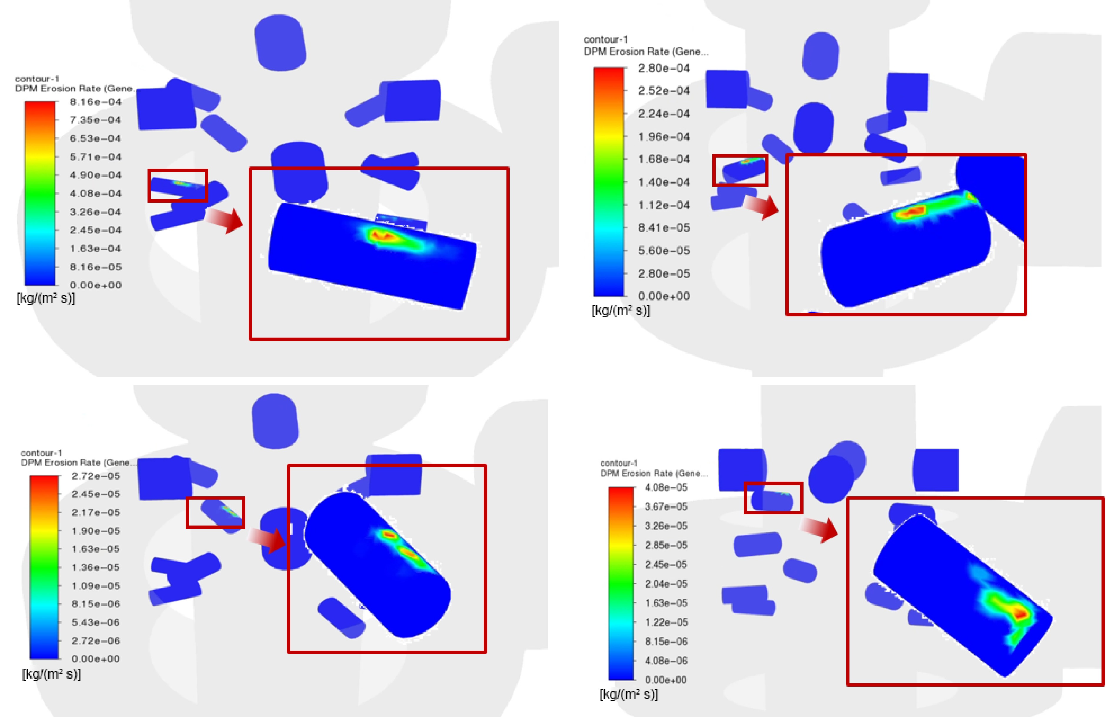
Figure 7. 

Erosion rate contours of the adjustable nozzle under different opening conditions.

As shown in Fig. 7, with increasing opening of the adjustable nozzle, the velocity distribution of the fluid gradually becomes more uniform, and the reduction in local high-velocity regions directly decreases the impact force exerted on the wall surface. As the opening increases, the flow field within the nozzle becomes more evenly distributed, resulting in reduced shear stress and fewer localized high-velocity zones. Consequently, the impact intensity on the wall is weakened, leading to a significant mitigation of erosion.

As shown in Fig. 8, with increasing nozzle opening, the erosion rate decreases from 8.16 × 10⁻⁴ kg/(m²·s) to 4.06 × 10⁻⁵ kg/(m²·s), indicating a significant reduction in erosion intensity. Meanwhile, the monthly erosion thickness decreases from 0.94 to 0.05 mm, demonstrating a substantial mitigation of erosive wear. These results suggest that appropriately increasing the opening of the adjustable nozzle can effectively reduce erosion caused by non-uniform flow velocity, thereby extending the service life of the equipment and improving the stability and reliability of the system.

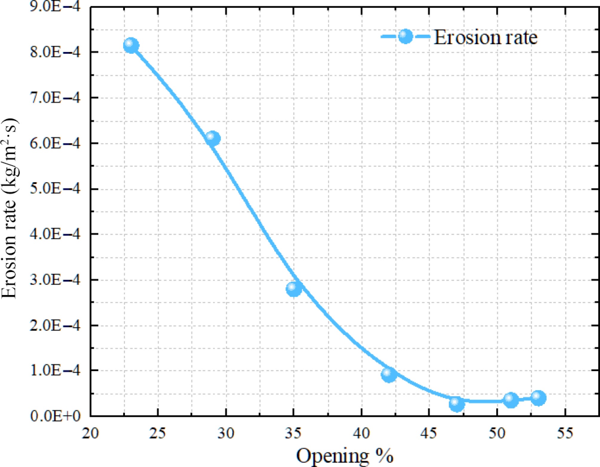
Figure 8. 

Effect of nozzle opening on the erosion rate.

3.2.2.   Erosive wear of the adjustable nozzle at different production pressure differentials

Based on the hourly production reports of Well HT101 and actual field operating conditions, the variation in erosion rate was investigated as the production pressure differential—defined as the difference between the upstream nozzle pressure and the downstream throttling pressure—increased from 20 to 50 MPa. The relationship between erosion rate and production pressure differential was obtained, as shown in Fig. 9.

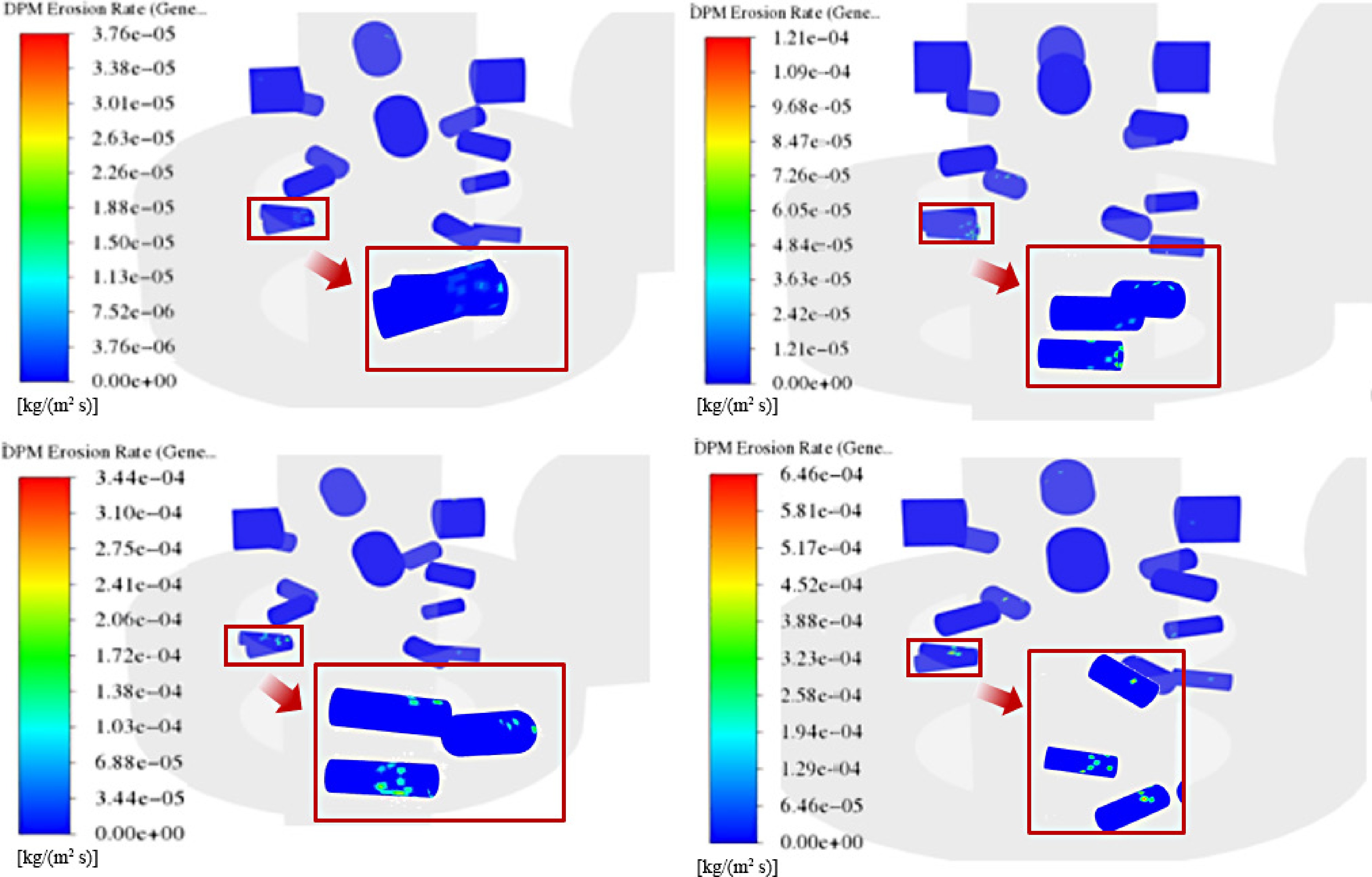
Figure 9. 

Erosion rate contours under different production pressure differentials.

As shown in Fig. 9, the scouring capability of the fluid increases significantly with increasing production pressure differential. This is attributed to the change in flow velocity and dynamic characteristics induced by a higher pressure differential, which enhances the impact force exerted on the solid surface and thereby intensifies the erosion process. As the pressure differential increases, the shear stress and kinetic energy of the fluid rise accordingly, leading to a higher erosion rate.

As shown in Fig. 10, with increasing production pressure differential, the erosion rate increases from 3.76 × 10⁻⁵ kg/(m²·s) to 6.46 × 10⁻⁴ kg/(m²·s), while the monthly erosion thickness rises from 0.04 to 0.74 mm. These results indicate that a higher pressure differential intensifies the long-term erosive wear on the solid surface, leading to a substantial increase in material loss. Therefore, the production pressure differential is a critical factor influencing fluid scouring intensity and material erosion resistance. Over prolonged operation, a significant increase in erosion thickness may result in premature equipment failure or performance degradation. Accordingly, effective protective and optimization measures should be implemented to mitigate erosion under high-pressure-differential conditions.

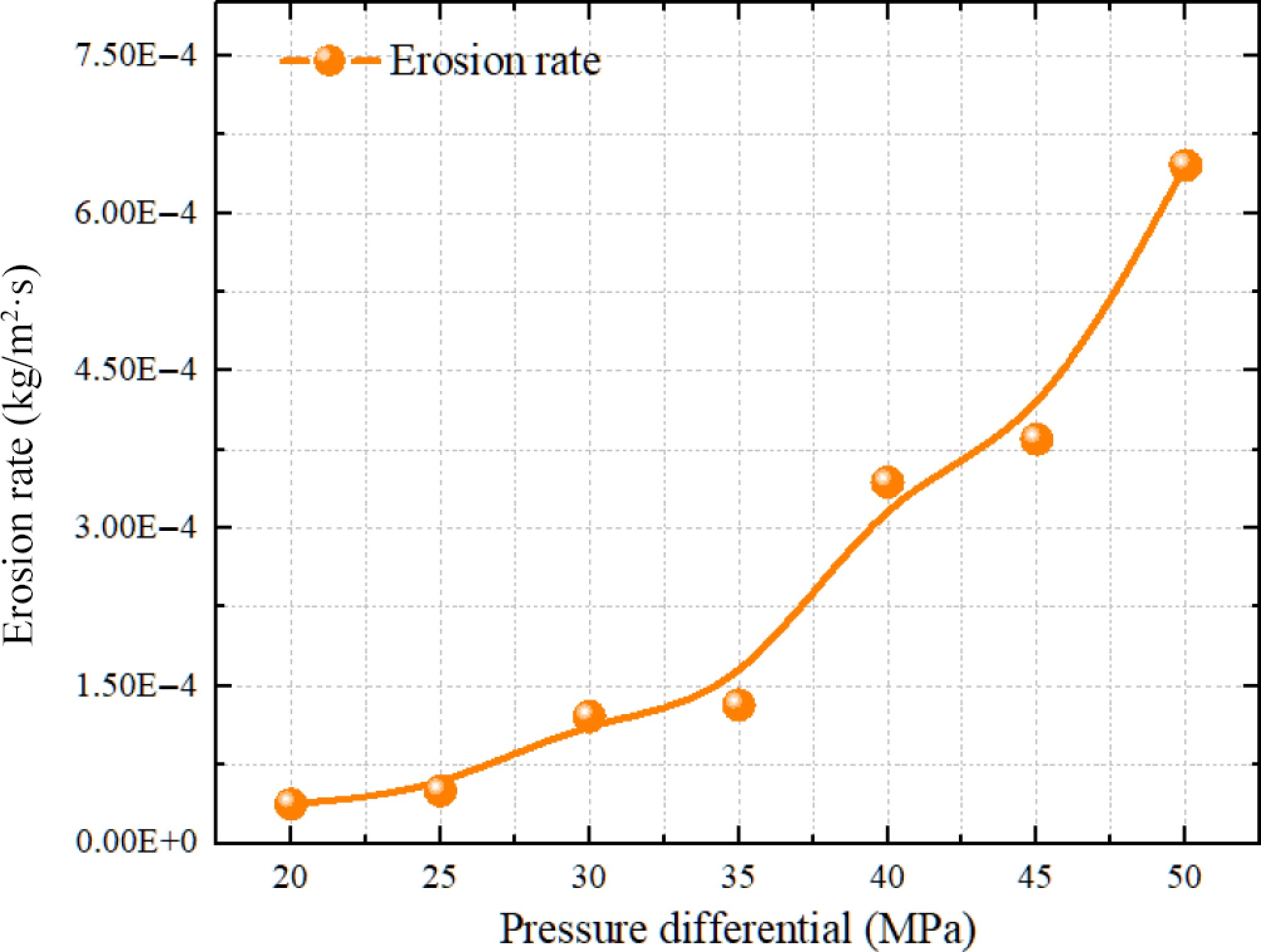
Figure 10. 

Effect of production pressure differential on the erosion rate.

3.2.3.   Erosive wear of the adjustable nozzle at different particle diameters

Based on the sand production data of Well HT101, the variation in erosion rate was investigated as the particle diameter increased from 25 to 50 μm. The relationship between erosion rate and particle diameter was subsequently obtained.

As shown in Fig. 11, with increasing particle diameter, the particle mass and inertia increase significantly, leading to a reduced ability to respond to variations in the fluid velocity field. Consequently, larger particles tend to maintain their original trajectories. In contrast, smaller particles, characterized by lower inertia and stronger flow-following capability, are more responsive to vortex structures and velocity gradients in the fluid. Under the effects of turbulent diffusion, vortex entrainment, and near-wall shear, they are more readily transported toward the wall region, resulting in a higher collision frequency per unit time. Therefore, as the particle size increases, the erosion rate decreases accordingly.

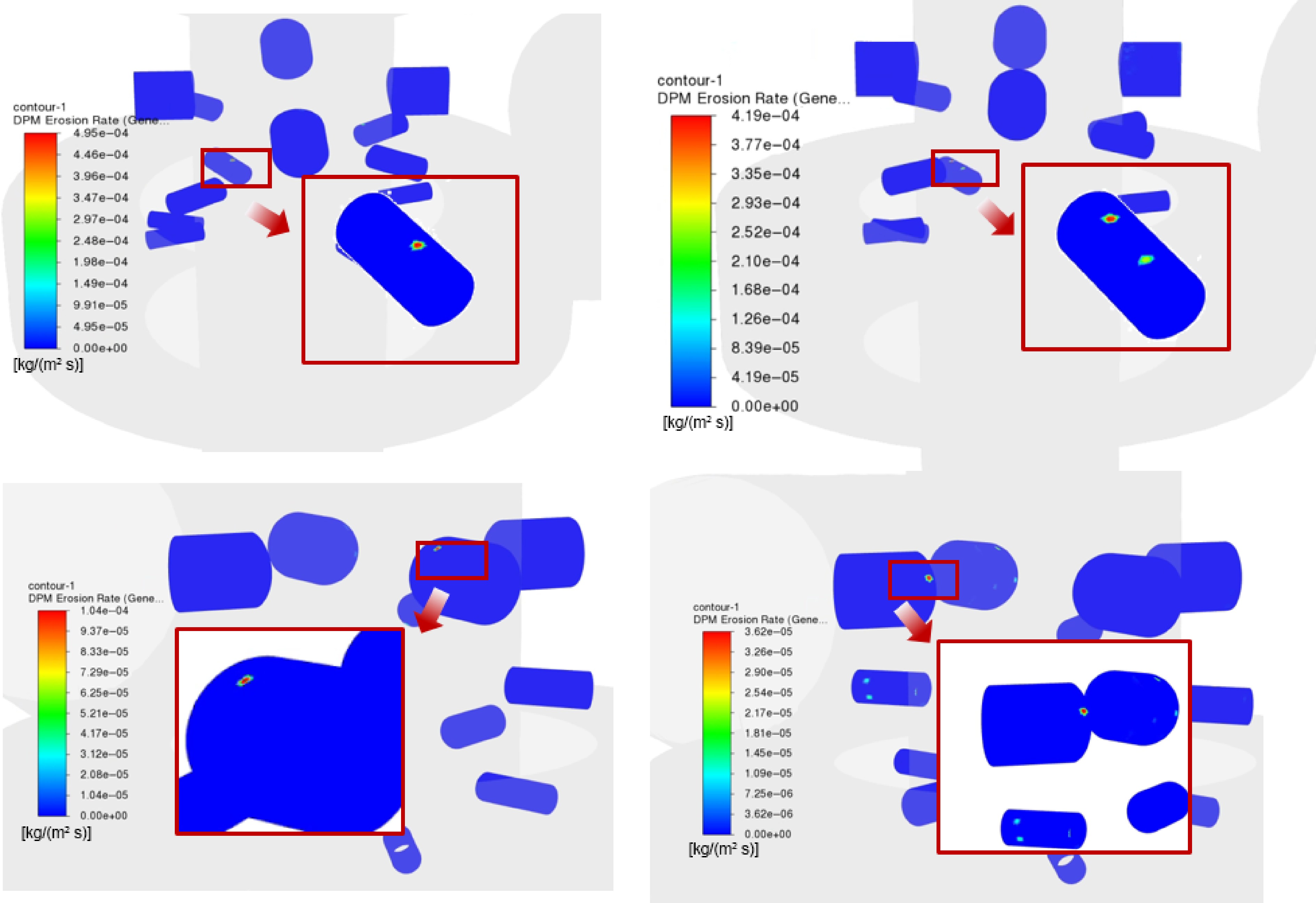
Figure 11. 

Erosion rate contours of the adjustable nozzle under different particle diameters.

As shown in Fig. 12, the erosion rate decreases significantly with increasing particle diameter, from 4.95 × 10⁻⁴ to 3.62 × 10⁻⁵ kg/(m²·s). Correspondingly, the monthly erosion thickness is reduced from 0.57 to 0.04 mm. These results indicate that variations in particle diameter alter the flow dynamics during the scouring process. Larger particles require greater impact energy to cause surface damage; however, due to the reduced collision frequency, the overall wall degradation is gradually mitigated. Therefore, in practical applications, controlling particle size can be an effective strategy to enhance equipment durability and reduce erosive wear losses.

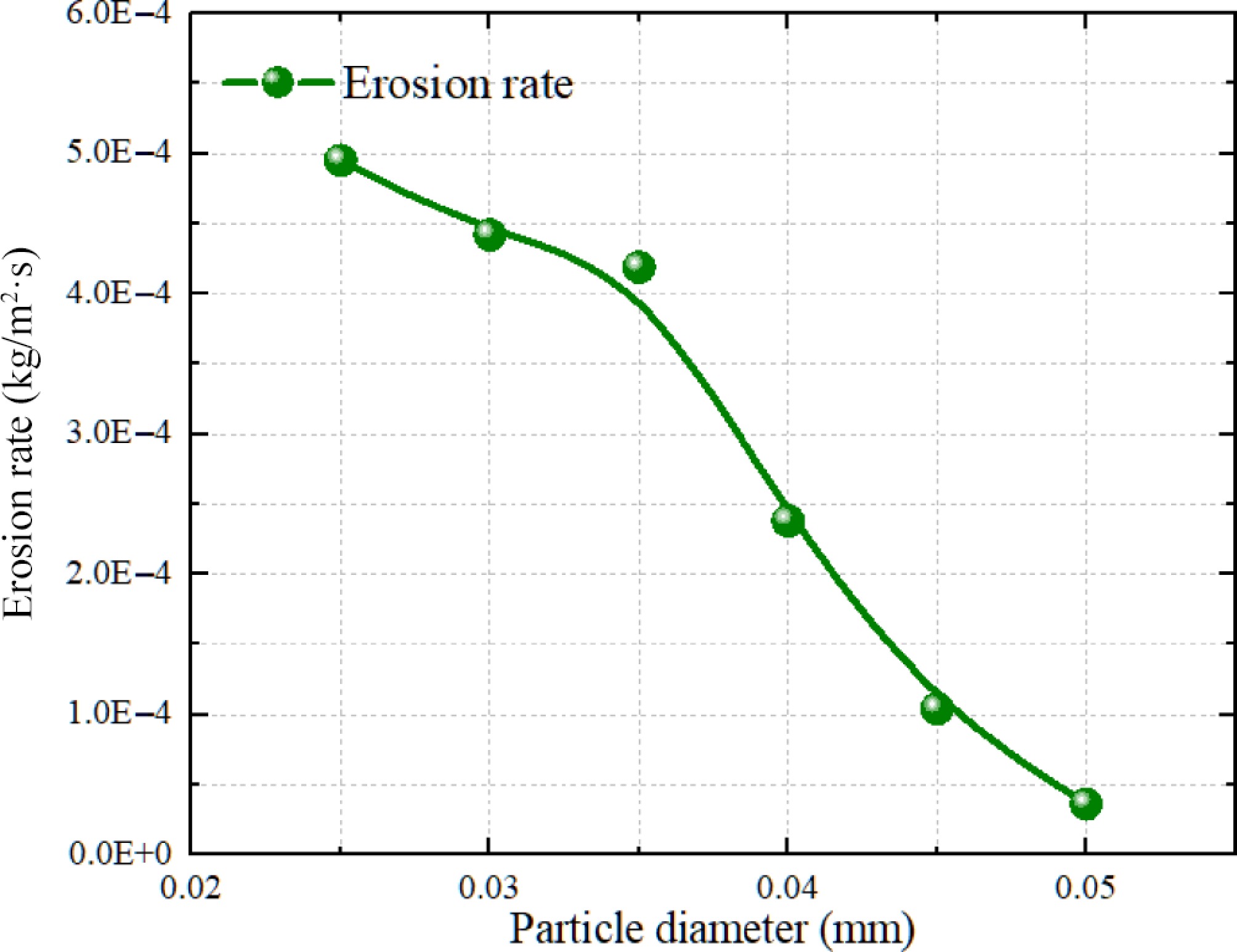
Figure 12. 

Effect of particle diameter on the erosion rate.

3.2.4.   Erosive wear of the adjustable nozzle at different particle densities

Based on the sand production conditions of Well HT101, the variation in erosion rate was investigated as the particle density increased from 2 to 2.8 g/cm³. The relationship between erosion rate and particle density was subsequently obtained.

As shown in Fig. 13, with increasing particle density, the mass and kinetic energy carried by solid particles per unit volume increase significantly. Under identical flow conditions, the impact intensity and destructive potential exerted on the wall surface are consequently enhanced. High-density particles transfer greater impact loads upon collision with the structural surface, making the material more susceptible to microcrack initiation and spalling, thereby aggravating the erosion process.

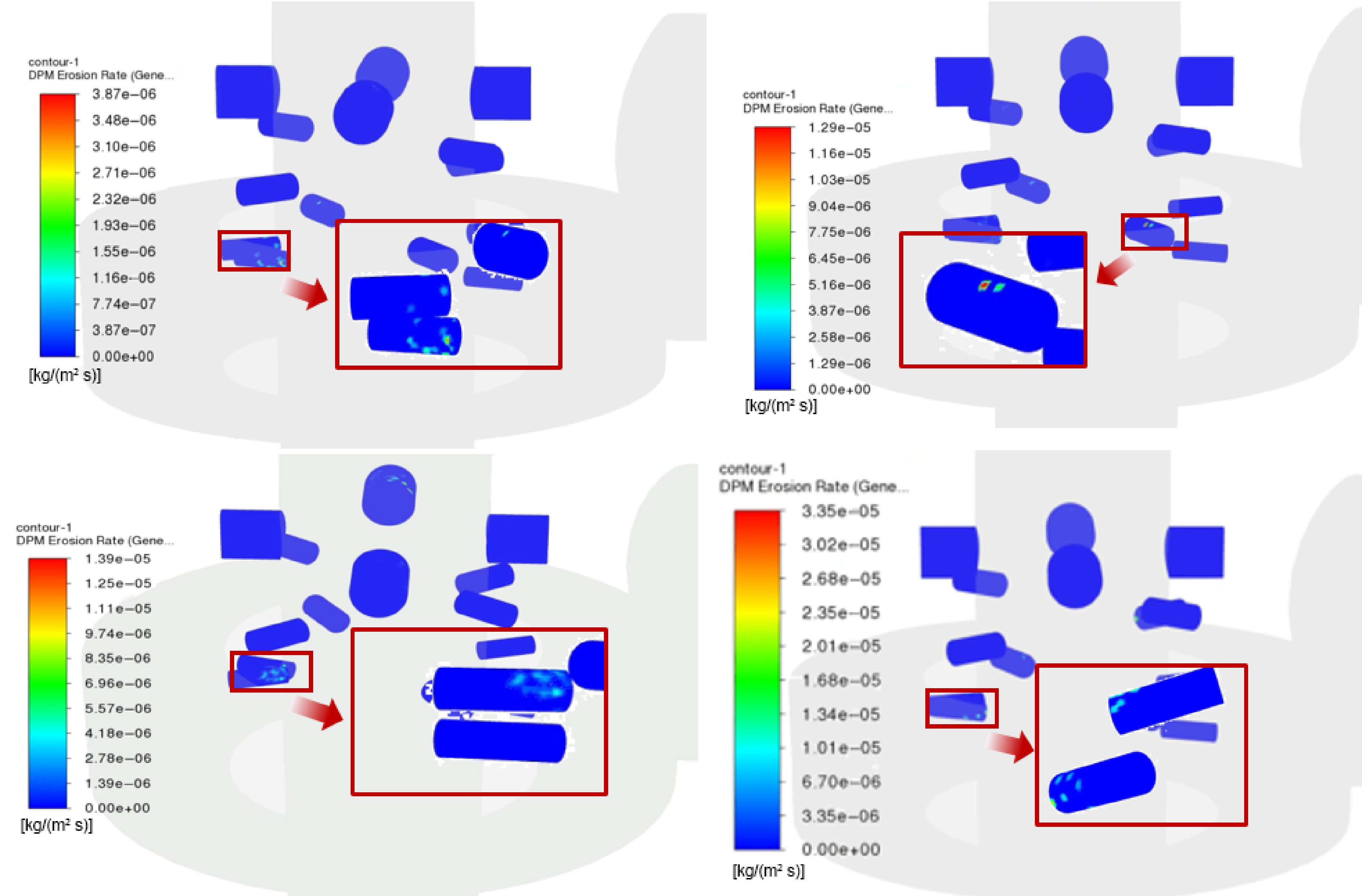
Figure 13. 

Erosion rate contours of the adjustable nozzle under different particle densities.

As shown in Fig. 14, the erosion rate increases markedly with increasing particle density, rising from 3.87 × 10⁻⁶ to 3.35 × 10⁻⁵ kg/(m²·s). Correspondingly, the monthly erosion thickness increases from 0.004 to 0.038 mm. These results indicate that, under long-term operating conditions, high-density particles exert a more pronounced cumulative damage effect on the inner wall of the equipment, leading to an accelerated material loss rate. Particle density is a key factor affecting erosion behavior. In ultra-high-pressure wellhead throttling operations, its influence on erosion risk should be considered to mitigate erosion damage.

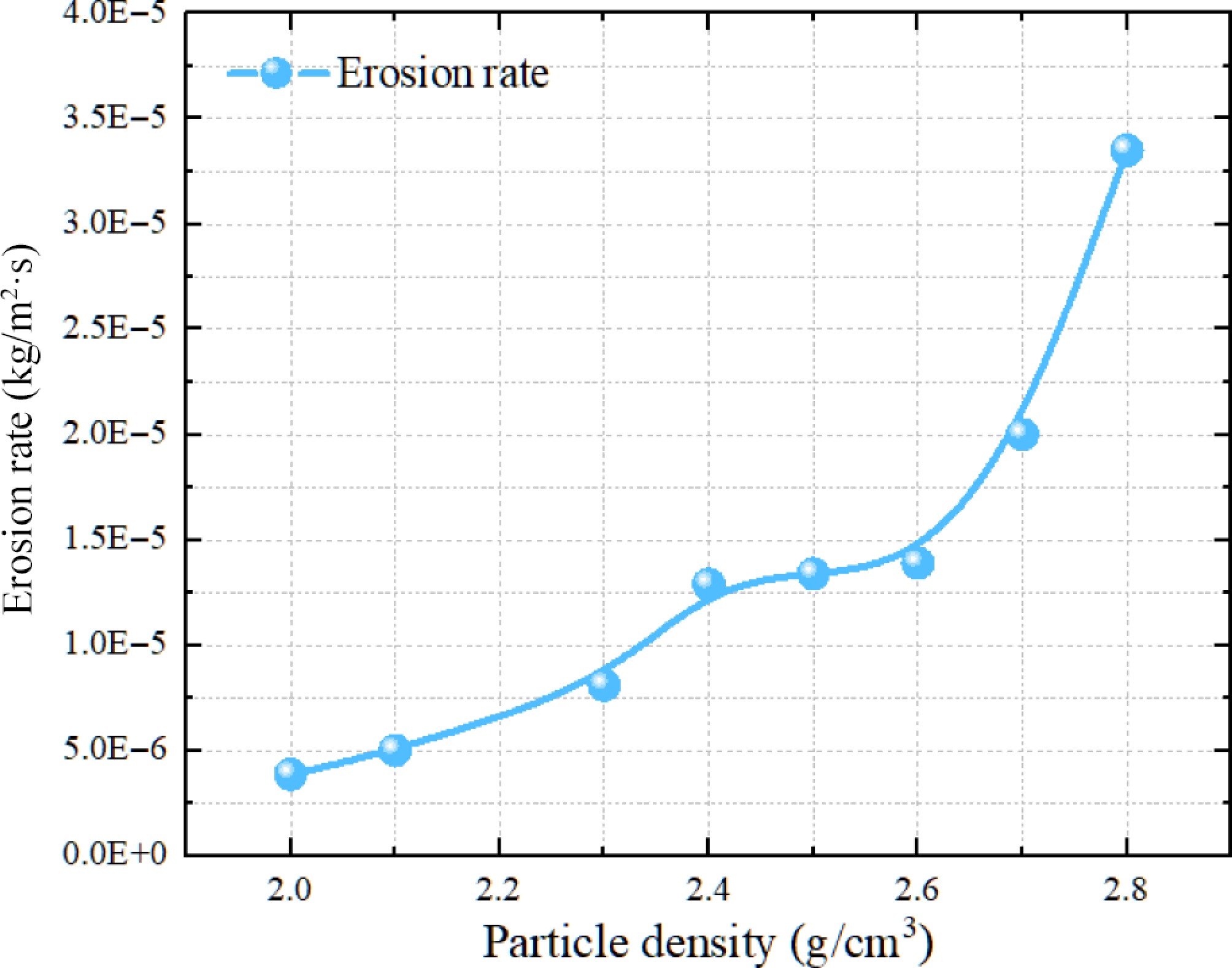
Figure 14. 

Effect of particle density on the erosion rate.

3.2.5.   Erosive wear of the adjustable nozzle at different sand production rates

Based on the sand production data of Well HT101, the variation in erosion rate was investigated as the sand production rate increased from 5 to 20 ml/d. The relationship between erosion rate and sand production rate was subsequently obtained.

As shown in Fig. 15, with increasing sand production rate, the number of solid particles in the particle-laden flow increases significantly, leading to a higher collision frequency and greater total kinetic energy imparted to the wall surface. The particle-laden flow not only carries the kinetic energy of the fluid itself but also transfers the kinetic energy of the particles to the wall, thereby intensifying the impact effect on the surface.

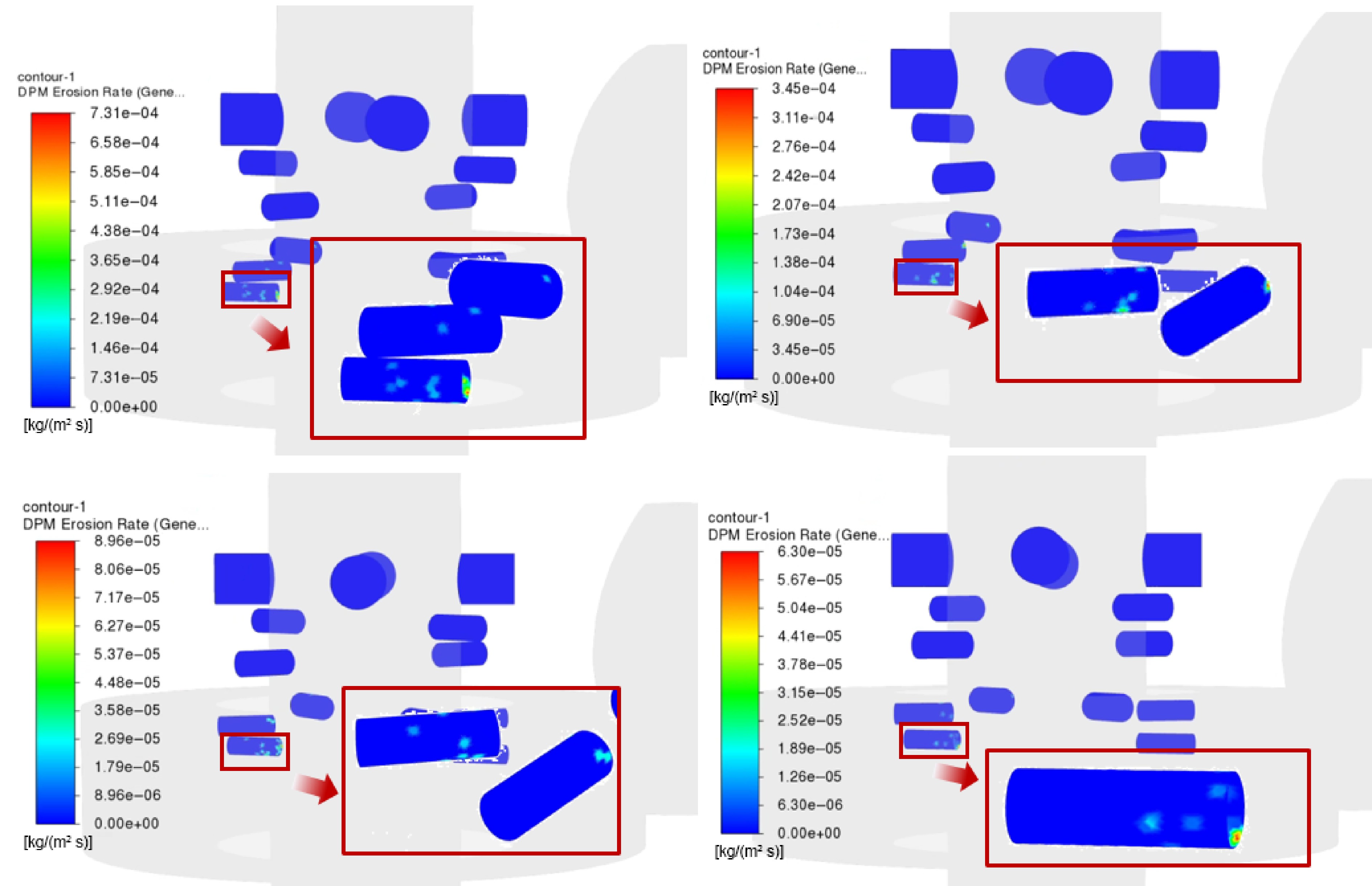
Figure 15. 

Effect of sand production rate on the erosion rate.

As shown in Fig. 16, the presence of particles leads to a more concentrated kinetic energy distribution in the flow and a substantial increase in impact frequency, resulting in a significant rise in the erosion rate. Specifically, the erosion rate increases from 6.3 × 10⁻⁵ to 7.3 × 10⁻⁴ kg/(m²·s), indicating markedly intensified erosion damage to the wall surface due to particle-laden flow. In addition, the monthly erosion thickness increases from 0.07 to 0.84 mm, demonstrating a pronounced increase in erosion depth with higher sand production rates. This phenomenon indicates that particle impingement exhibits a cumulative effect, with erosion severity increasing as the sand production rate rises. Therefore, the proper application of desanders in surface throttling processes can effectively mitigate erosion damage, extend equipment service life, and ensure stable system operation.

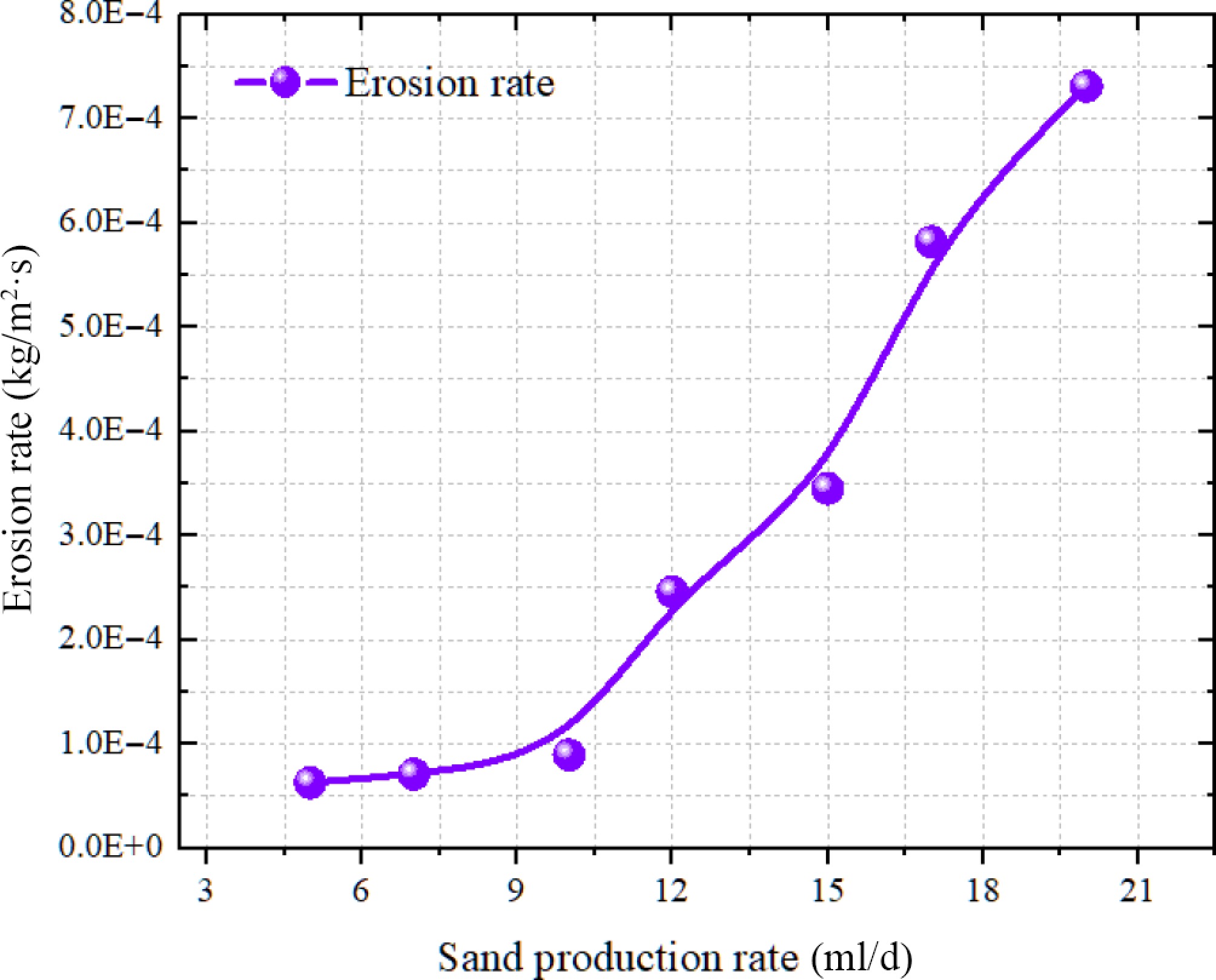
Figure 16. 

Effect of sand production rate on the erosion rate.

3.2.6.   Sensitivity analysis under orthogonal experimental design

In the single-factor experiments, each variable was independently controlled and analyzed to investigate its individual effect on the results. Although this approach can reveal the influence of a single factor, it does not account for potential interaction effects among multiple factors. To achieve an efficient and systematic analysis of multi-factor influences, this study adopts an orthogonal experimental design based on the principles of Design of Experiments (DoE) and the Taguchi method. Orthogonal arrays enable balanced combinations of factor levels with statistical independence, allowing the main effects of multiple variables to be estimated with a reduced number of experiments, thereby significantly lowering experimental or computational costs.

In this study, the evaluation index is the monthly erosion thickness converted from the maximum erosion rate. Based on the preceding single-factor analysis of nozzle erosion, five primary influencing factors were identified: production pressure differential, sand production rate, particle diameter, particle density, and nozzle opening. Considering that five independent variables are involved, each with five levels, a full factorial design would require 3,125 experiments, which is computationally expensive and impractical. Therefore, an L25 (5⁵) orthogonal array was selected, requiring only 25 experimental runs while ensuring uniform distribution and comparability of factor levels, thus guaranteeing the representativeness and reliability of the results.

It should be noted that orthogonal experimental design primarily focuses on the analysis of main effects and has limited capability in capturing higher-order interactions. Nevertheless, due to its high efficiency, robustness, and suitability for multi-factor screening and sensitivity analysis, this method has been widely applied in engineering studies.

As shown in Table 2, five factors—production pressure differential, particle diameter, particle density, nozzle opening, and sand production rate—were selected as the variables of interest. An orthogonal experiment was designed based on the L₂₅5⁵ orthogonal array. The experimental scheme and corresponding results are presented in Table 3.

As shown in Table 3, the minimum erosion rate occurs when the production pressure differential is 20 MPa, the particle diameter is 35 μm, the nozzle opening is 35%, the sand production rate is 15 ml/d, and the particle density is 2.4 g/cm³, with a monthly erosion thickness of only 0.005 mm. Conversely, the maximum erosion rate is observed when the production pressure differential is 35 MPa, the particle diameter is 35 μm, the nozzle opening is 23%, the sand production rate is 20 ml/d, and the particle density is 2.8 g/cm³, resulting in a monthly erosion thickness of 3.75 mm.

To more intuitively clarify the influence of each factor on the maximum erosion rate of the nozzle, a range analysis was conducted to determine the relative significance of each factor. The results of the range analysis are presented in Table 4.

As shown in Table 4, k₁, k₂, k₃, k₄, and k₅ represent the average results of the three experimental runs for production pressure differential, particle diameter, nozzle opening, particle density, and sand production rate, respectively, while R denotes the range.

As shown in Fig. 17, to more clearly analyze the results of the orthogonal experiment, a plot of factor levels versus response trends and a bar chart of factor ranges were drawn. The range analysis results indicate that the influence of the factors on nozzle erosion follows the order: nozzle opening > sand production rate > particle density > production pressure differential > particle diameter. Specifically, nozzle opening and sand production rate have the most significant impact on the nozzle erosion rate, highlighting their dominant role in the erosion process. In contrast, particle diameter has a relatively minor effect, suggesting that in practical applications, the main driving factors of nozzle erosion are closely associated with nozzle opening and sand production rate. The range analysis provides a quantitative assessment of each factor's contribution to the erosion rate, offering a scientific basis for optimizing nozzle design and operating parameters, and enabling more effective control of erosion in practice.

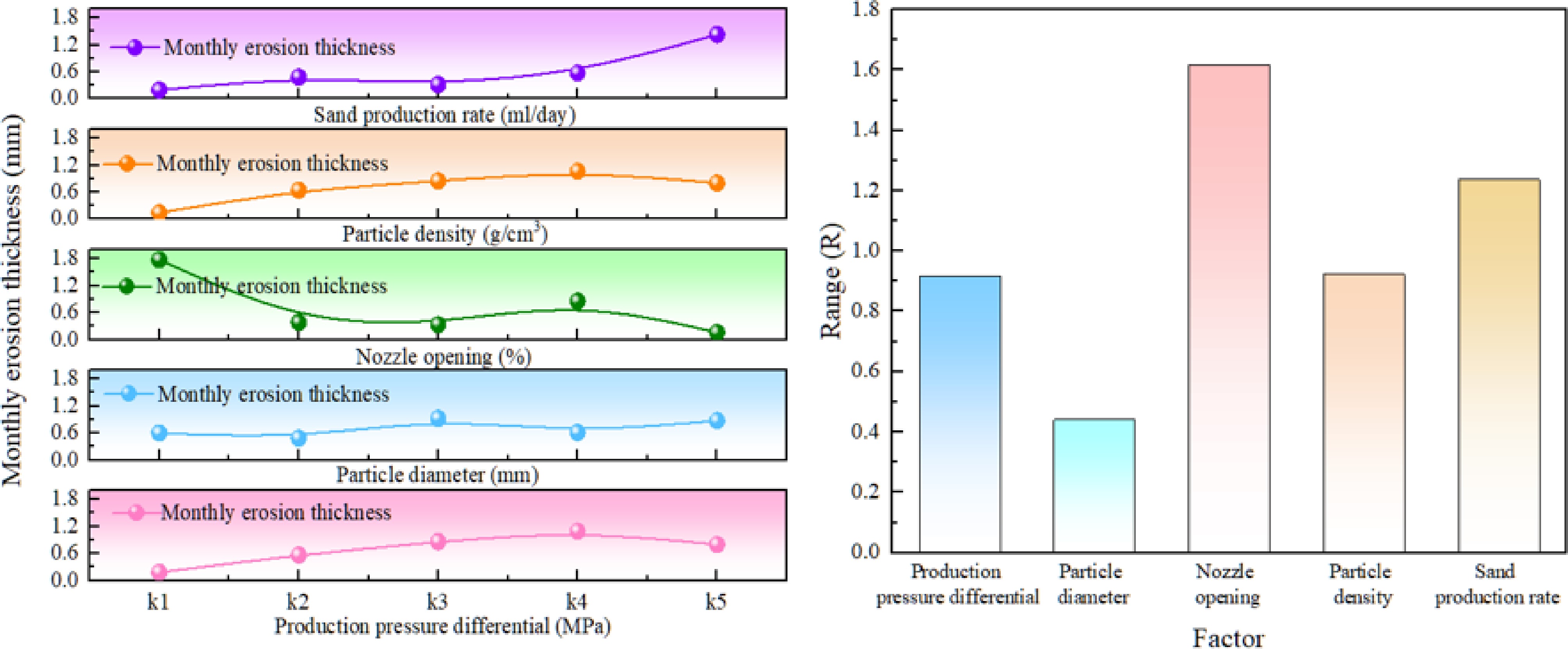
Figure 17. 

Range analysis results.

3.3.   Analysis of nozzle erosion prediction model

3.3.1.   Dataset and feature correlation analysis

Based on the hourly reports of well HT101, 186 data sets were compiled after removing duplicate entries. The input variables included production pressure differential (the difference between the upstream pressure at the nozzle inlet and the downstream pressure at the nozzle outlet), nozzle opening, sand production rate, particle density, and particle diameter. The erosion rate, calculated using Fluent software, was taken as the target variable.

In addition, when selecting input features for data-driven modeling, severe multicollinearity among features can often lead to overfitting and biased parameter estimates. Therefore, to verify the rationality of the selected features, a feature correlation analysis is usually conducted. Pearson and Spearman correlation coefficients are widely used to quantify the relationships between continuous variables. Compared with the Pearson correlation coefficient, which primarily characterizes linear relationships and typically relies on the assumption of normally distributed variables, the Spearman correlation coefficient is a rank-based non-parametric method that does not impose strict requirements on data distribution and is more robust to outliers. More importantly, it is capable of capturing monotonic relationships between variables, including nonlinear but monotonic trends.Given that the relationships between input features and erosion rate in this study may exhibit nonlinearity and deviate from normality, the use of the Spearman correlation coefficient provides a more appropriate and robust characterization of feature correlations. The Spearman correlation coefficient can be approximately calculated using the following formula^[39]:

In the formula, d_i represents the rank difference of the corresponding variable, i.e., the difference between the ranks of paired samples after sorting the two variables; n is the sample size (or the total number of observations); and ρ_s denotes the Spearman correlation coefficient. The closer the absolute value of ρ_s is to 1, the stronger the correlation between the variables.

As shown in Fig. 18, a feature correlation analysis was conducted for production pressure differential (p), choke opening (k), particle diameter (d), sand production rate (Q), and particle density (ρ). In general, variables exhibiting high correlation (|ρ_s| ≥ 0.8) are not recommended to be simultaneously used as input variables^[39]. When variables exhibit high correlation (|ρ_s| ≥ 0.8), they often introduce redundant information and potential multicollinearity, which may adversely affect model stability, interpretability, and generalization performance; therefore, they are not recommended to be included simultaneously. The Spearman correlation matrix indicates that sand production (Q) exhibits a strong positive correlation with pressure differential (p, ρ_s = 0.76) and particle diameter (d, ρ_s = 0.58), while showing a moderate negative correlation with nozzle opening (k, ρ_s = −0.58) and particle density (ρ, ρ_s = −0.35). Here, the strength of correlation is evaluated based on the absolute value of ρ_s, where |ρ_s| < 0.3, 0.3 ≤ |ρ_s| < 0.7, and |ρ_s| ≥ 0.7 correspond to weak, moderate, and strong correlations, respectively. The inter-feature correlations remain moderate (< 0.4), suggesting the absence of severe multicollinearity.

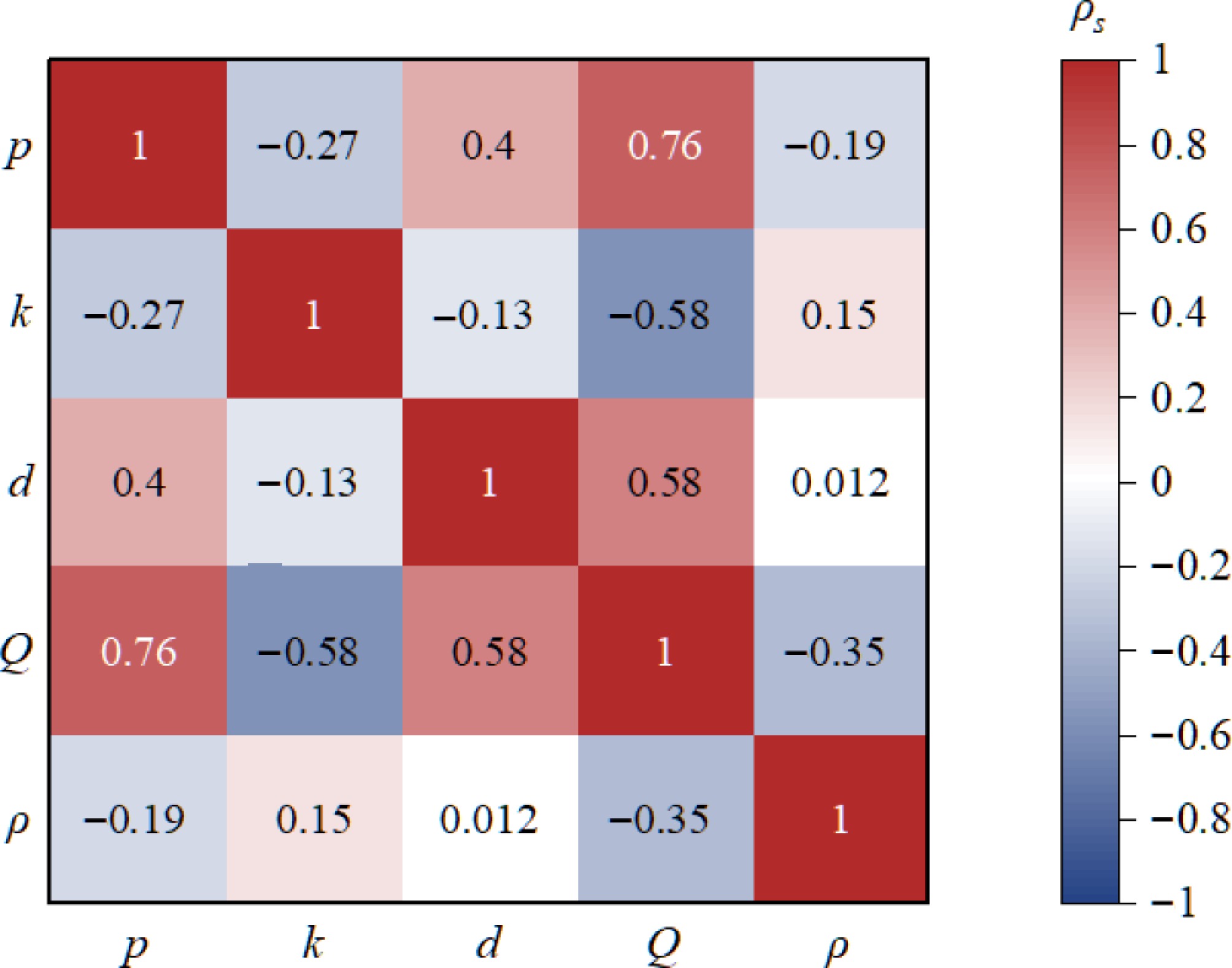
Figure 18. 

Feature correlation analysis

3.3.2.   Analysis of predictive model results

To emphasize the development of the GPR model and to comparatively examine the influence of different kernel functions on predictive performance, this study follows the GPR construction procedure described above. Specifically, the training set was modeled using the RBF, Matérn, and rational quadratic kernels, respectively, and the resulting models were subsequently evaluated on the test set to assess and compare their predictive performance. It should be noted that the comparison of different kernel functions is not merely a technical performance evaluation, but is intended to identify the most suitable knowledge representation and modeling structure for this complex engineering problem. In doing so, it helps reveal the underlying functional characteristics and inherent patterns of the erosion process, thereby improving the physical consistency and generalization capability of the model.

As shown in Fig. 19, a systematic comparison was conducted to identify the optimal kernel mechanism for the GPR-based erosion-rate prediction model, considering the RBF (radial basis), Matérn, and rational quadratic kernels. Based on 149 experimental samples, the rational quadratic kernel achieved the highest fitting accuracy and demonstrated superior generalization potential, primarily due to its enhanced capability in capturing multi-scale correlation structures. Specifically, it yielded an R² of 0.962, markedly outperforming the Matérn (0.941) and RBF (0.895) kernels.To further mitigate partition-induced uncertainty and rigorously assess model stability, 5-fold cross-validation was performed on the training dataset. The results show that the rational quadratic kernel consistently maintains strong predictive performance across folds, with an average R² of 0.91 ± 0.02 and limited variability. Compared to the training performance (R² = 0.962), no substantial degradation is observed, indicating that the model does not exhibit pronounced overfitting and retains stable predictive behavior.

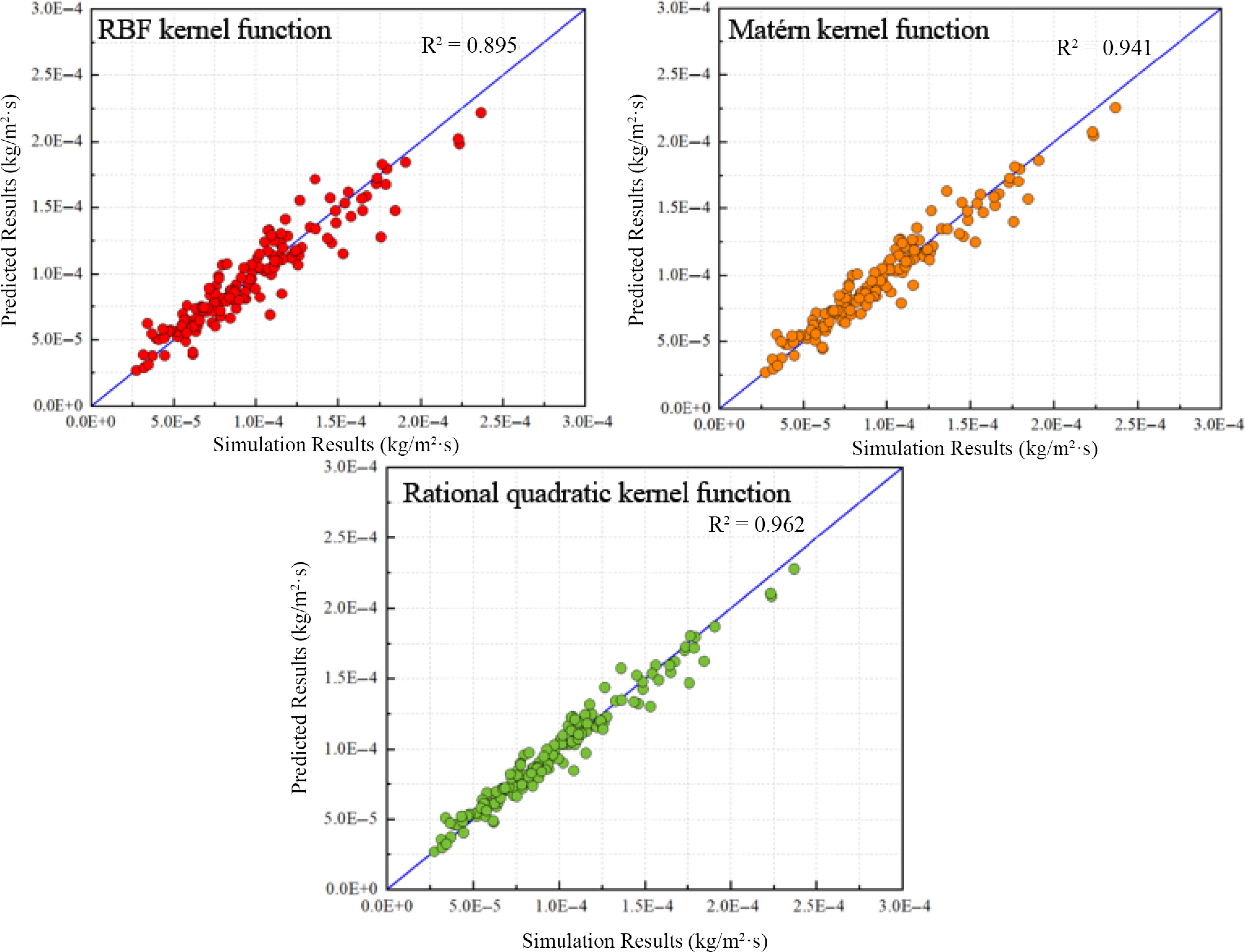
Figure 19. 

Predicted erosion-rate results for the training set.

Nevertheless, to more rigorously evaluate generalization under unseen conditions, an independent test set was employed for extrapolative validation, ensuring robust predictive reliability beyond the training domain.

As shown in Fig. 20, an independent test set was employed to validate the GPR prediction models with different kernel functions. Fig. 19 presents not only the simulated values and the predicted means of the samples, but also the corresponding 95% confidence intervals.

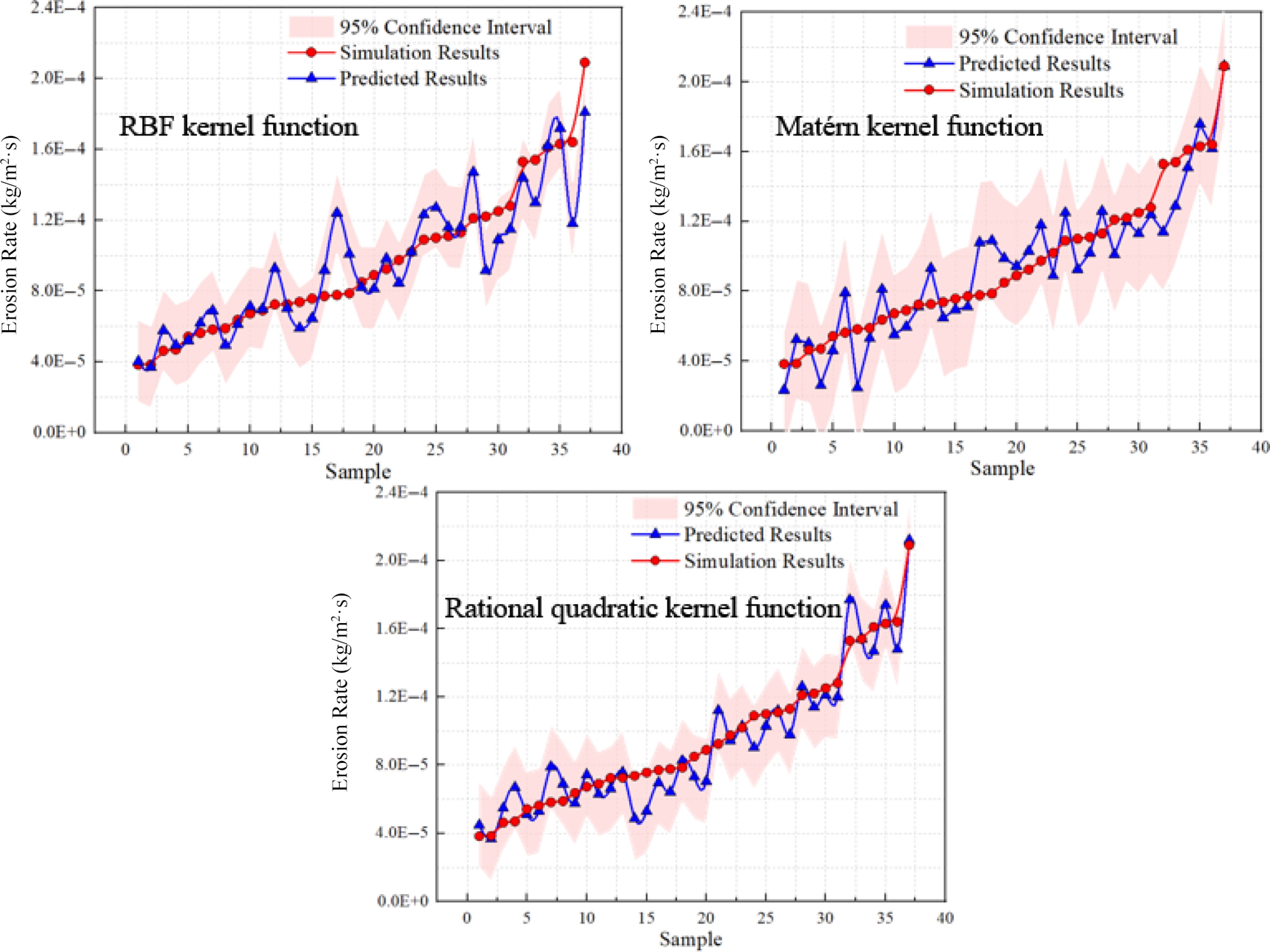
Figure 20. 

Predicted erosion-rate results.

For the GPR model predicting the erosion rate, when the radial basis function (RBF) kernel was adopted, the maximum absolute error reached 4.64 × 10⁻⁵ kg/(m²·s), and four samples fell outside the 95% confidence interval. When the Matérn kernel was used, the maximum absolute error decreased to 3.9 × 10⁻⁵ kg/(m²·s), with only two samples lying outside the 95% confidence interval. In contrast, when the rational quadratic kernel was employed, the maximum absolute error was further reduced to 2.5 × 10⁻⁵ kg/(m²·s), and all samples were contained within the 95% confidence interval.

As shown in Table 5, the coefficients of determination (R²) for the RBF, Matérn, and rational quadratic kernels are 0.835, 0.829, and 0.910, respectively. The GPR model constructed with the rational quadratic kernel exhibits the closest agreement between the predicted mean values and the simulated results, achieving the lowest RMSE and the highest R², which are 1.21 × 10⁻⁵ and 0.910, respectively.

Overall, for the dataset considered in this study, the GPR model employing the rational quadratic kernel demonstrates the best generalization performance. It ensures relatively small prediction errors while producing narrower confidence intervals compared with the other two kernel functions. Therefore, it is recommended to adopt the rational quadratic kernel for constructing the GPR model to predict the nozzle erosion rate.

Through a systematic investigation of the erosion and wear characteristics of surface throttling in ultra-high-pressure condensate gas wells, as well as the associated prediction models, the following conclusions can be drawn:

(1) Under ultra-high-pressure operating conditions, analysis of the erosion contour of the CV10 adjustable nozzle indicates that the regions most susceptible to erosion on the valve core are primarily concentrated on the backflow surface and at the outlet of the lateral flow surface. Among these, the lateral flow surface experiences the most severe erosion, whereas no significant erosion is observed on the inner wall of the valve core. These findings are generally consistent with field operational observations. Meanwhile, a certain degree of erosion wear is also observed on the valve sleeve; however, its severity is markedly lower than that of the valve core. The underlying mechanisms require further in-depth investigation in future studies. From an engineering application perspective, the above erosion distribution characteristics indicate that the lateral flow surface of the valve core is more prone to wall thinning, thereby becoming a critical region affecting equipment service life and potential failure risk. This area should be prioritized for monitoring and evaluation during actual operation and maintenance.

(2) For the surface CV10 throttling nozzle used in ultra-high-pressure condensate gas wells, when the wellhead pressure ranges from 75 to 130 MPa and the sand production rate is 5–20 ml/d. Increasing the opening of the adjustable nozzle and reducing the production pressure differential of the gas well can effectively mitigate nozzle erosion. For every 10% increase in nozzle opening, the erosion rate decreases by an average of 1.97 × 10⁻⁴ kg/(m²·s), and the monthly erosion thickness is reduced by approximately 0.23 mm. For every 5 MPa reduction in production pressure differential, the erosion rate decreases by an average of 7.66 × 10⁻⁵ kg/(m²·s), and the monthly erosion thickness is reduced by approximately 0.08 mm.

(3) Under ultra-high-pressure conditions, the relative influence of different factors on the erosion of the adjustable nozzle follows the order: nozzle opening > sand production rate > particle density > production pressure differential > particle size. A reduction in nozzle opening significantly aggravates erosion. The sand production rate affects both the frequency and intensity of particle impingement. Although particle density, production pressure differential, and particle size exert comparatively smaller effects, their influence remains non-negligible. Therefore, these factors should be comprehensively considered in the optimization of nozzle design to extend its service life.

(4) Regarding the erosion prediction model, a Gaussian Process Regression (GPR)-based model was developed to predict nozzle erosion, and three different kernel functions were comparatively evaluated. The coefficients of determination (R²) for the RBF, Matérn, and rational quadratic kernels are 0.835, 0.829, and 0.910, respectively. The GPR model constructed with the rational quadratic kernel shows the closest agreement between predicted and simulated values, achieving the minimum RMSE (1.21 × 10⁻⁵) and the maximum R² (0.910). Therefore, the GPR model employing the rational quadratic kernel demonstrates the best generalization performance among the considered kernels.