-
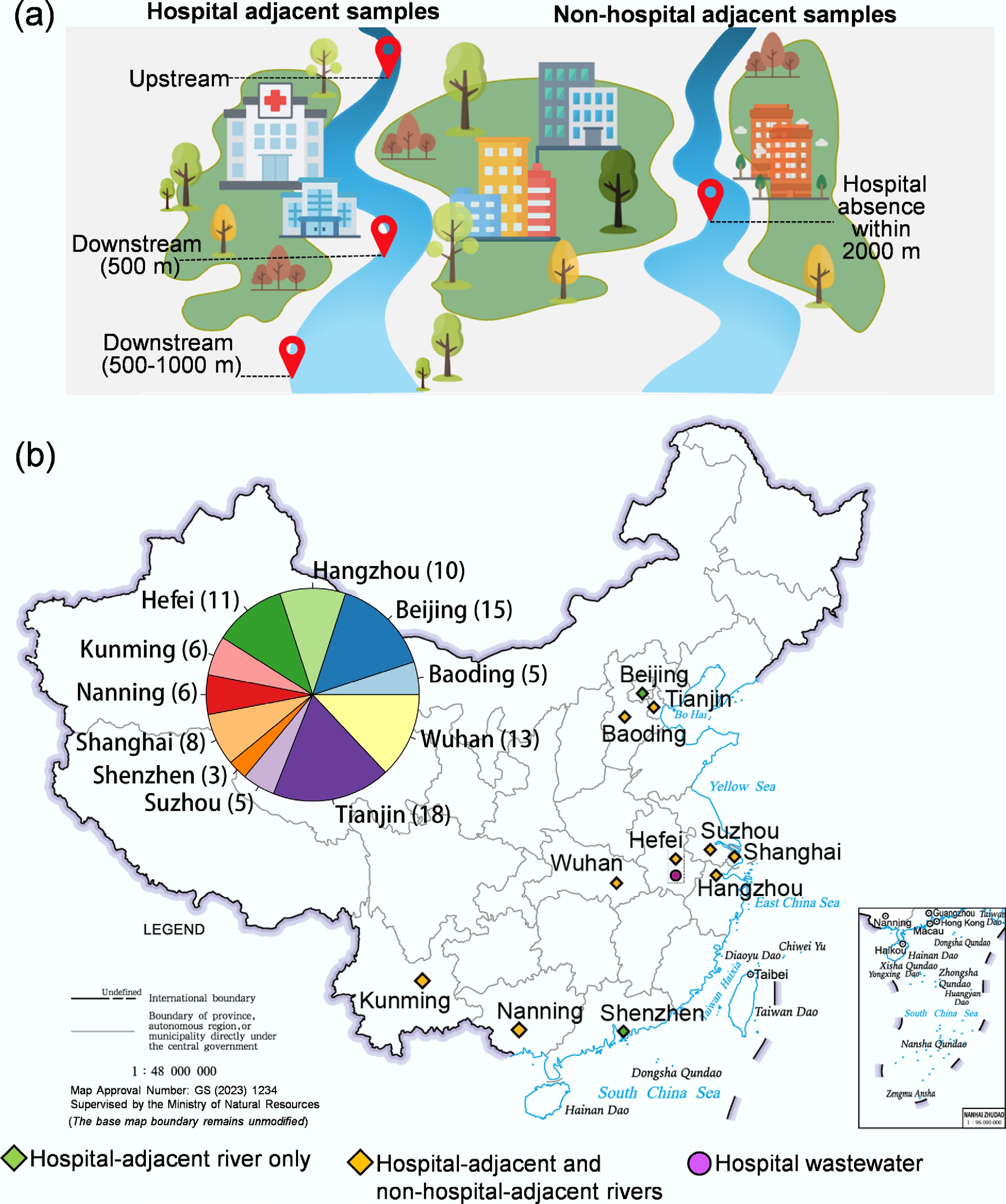
Figure 1.
Sampling design and geographical distribution of sampling sites. (a) Conceptual diagram illustrating the sampling strategy. (b) Geographical distribution of sampling sites across provinces and cities (blue shaded area). Symbol shapes and colors denote the sample types collected from the cities.
-
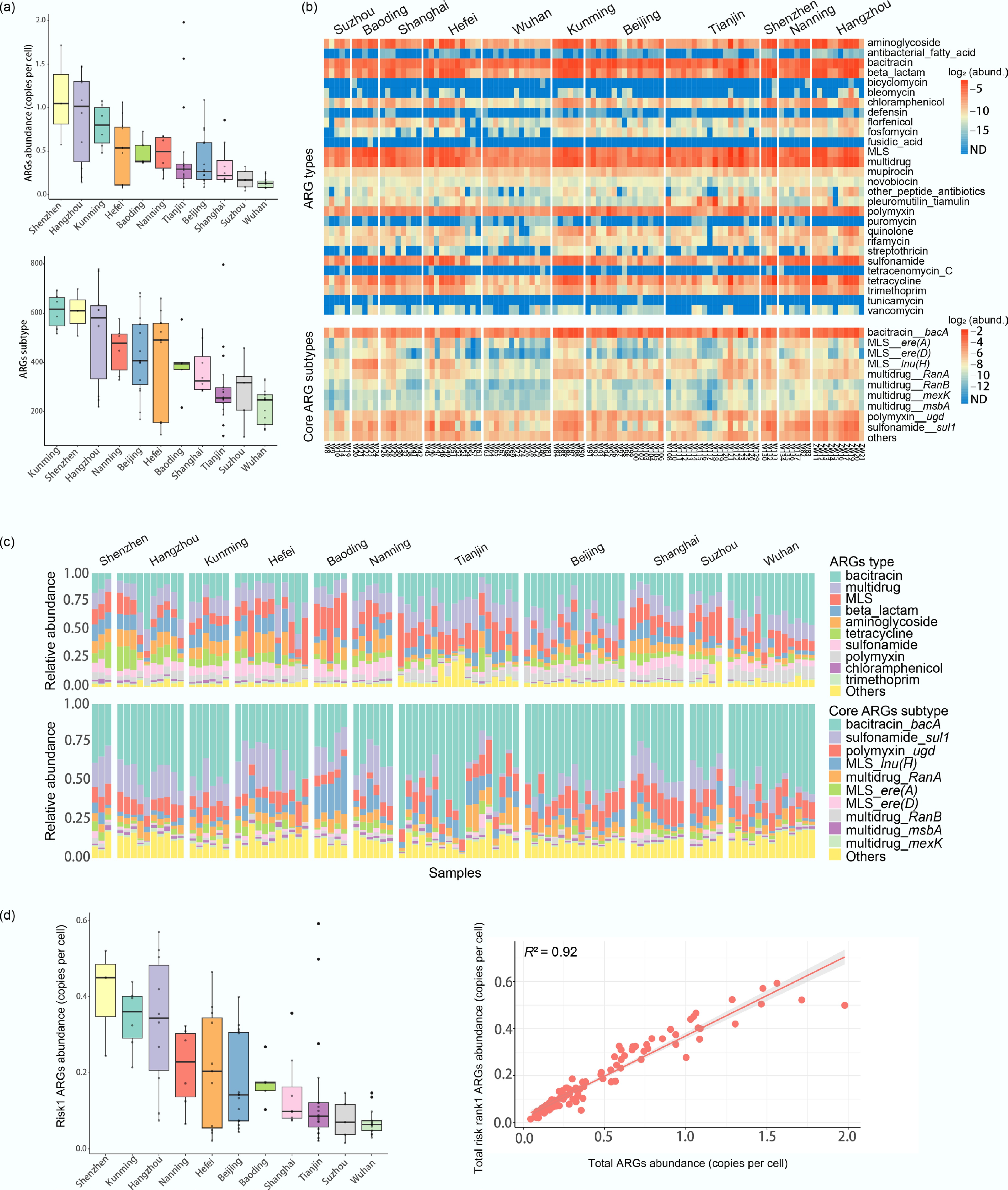
Figure 2.
Profiles of ARG abundance and diversity across samples. (a) Box plots of ARG abundance (copies per cell) and diversity (number of unique ARG subtypes) among the sampling cities (center line: median; box limits: 1st and 3rd quartiles). (b) Heatmap of the top 10 most dominant and core ARG subtypes. Abundance is displayed as log2-transformed copies per cell, with an offset of 1/10 of the minimum non-zero value added to each measurement to permit log transformation. (c) Compositional profiles of ARG types and core subtypes. The top 10 are labeled, with the remainder grouped as 'Others'. (d) Abundance of risk Rank 1 ARGs and the linear correlation between total ARGs and Risk I ARG abundances (p < 0.01).
-
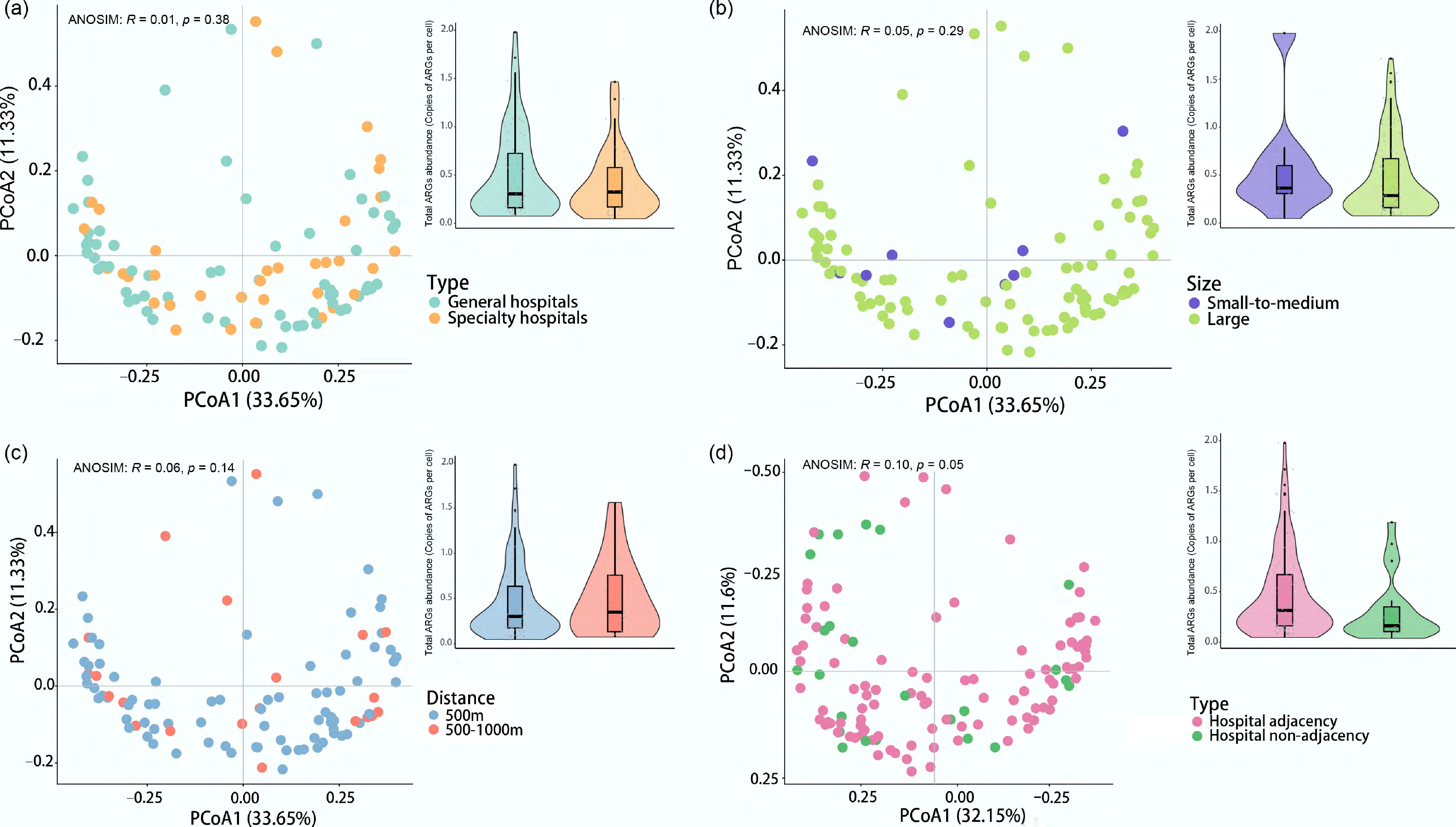
Figure 3.
Influence of hospital characteristics and proximity on the ARG profile. Panels show the effect of (a) hospital type (general vs specialty), (b) hospital size (large: > 500 beds; small-to-medium: 100–500 beds), (c) sampling distance downstream (near: ≤ 500 m; far: 500–1,000 m), and (d) hospital adjacency (hospital present within 2,000 m; hospital absent). In each panel, the right plot is a PCoA showing ARG profile clustering, and the left plot illustrates ARG abundance (copies per cell) as a boxplot (center line: median; box limits: 1st and 3rd quartiles).
-
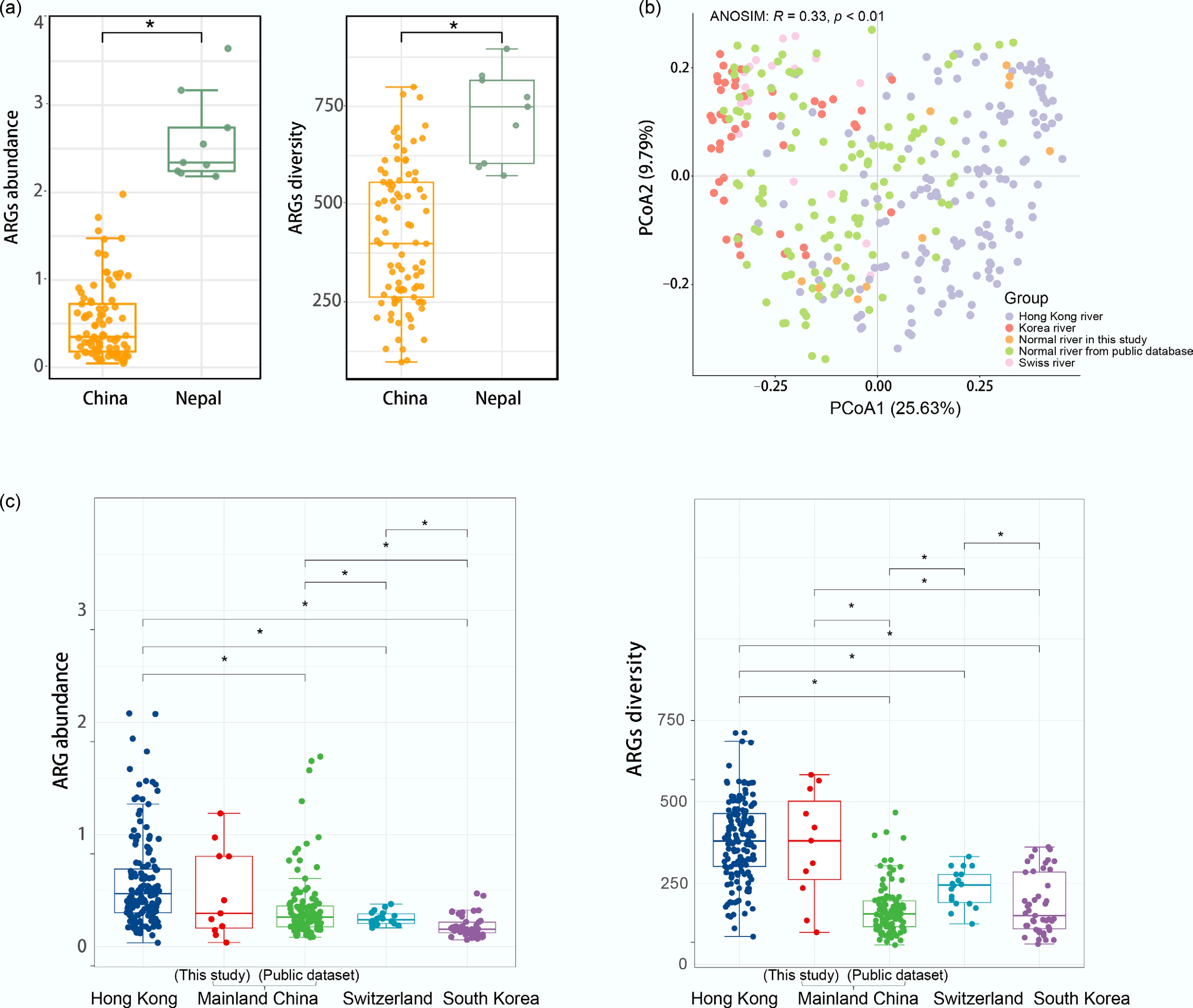
Figure 4.
Comparative analysis of ARG profiles across different geographical regions. (a) ARG abundance and diversity in hospital-adjacent rivers from China and Nepal. (b) PCoA plot based on Bray–Curtis dissimilarity, showing the overall similarity of ARG profiles in typical rivers among the different regional groups, including Mainland China (this study and public dataset[40]), Hong Kong[13], South Korea[41], and Switzerland[42]. (c) ARG abundance and diversity in typical rivers from different regional groups. In both panels, boxplots display the median (center line) and interquartile range (box). Significant differences between groups, determined by t-test, are indicated by asterisks (*).
-
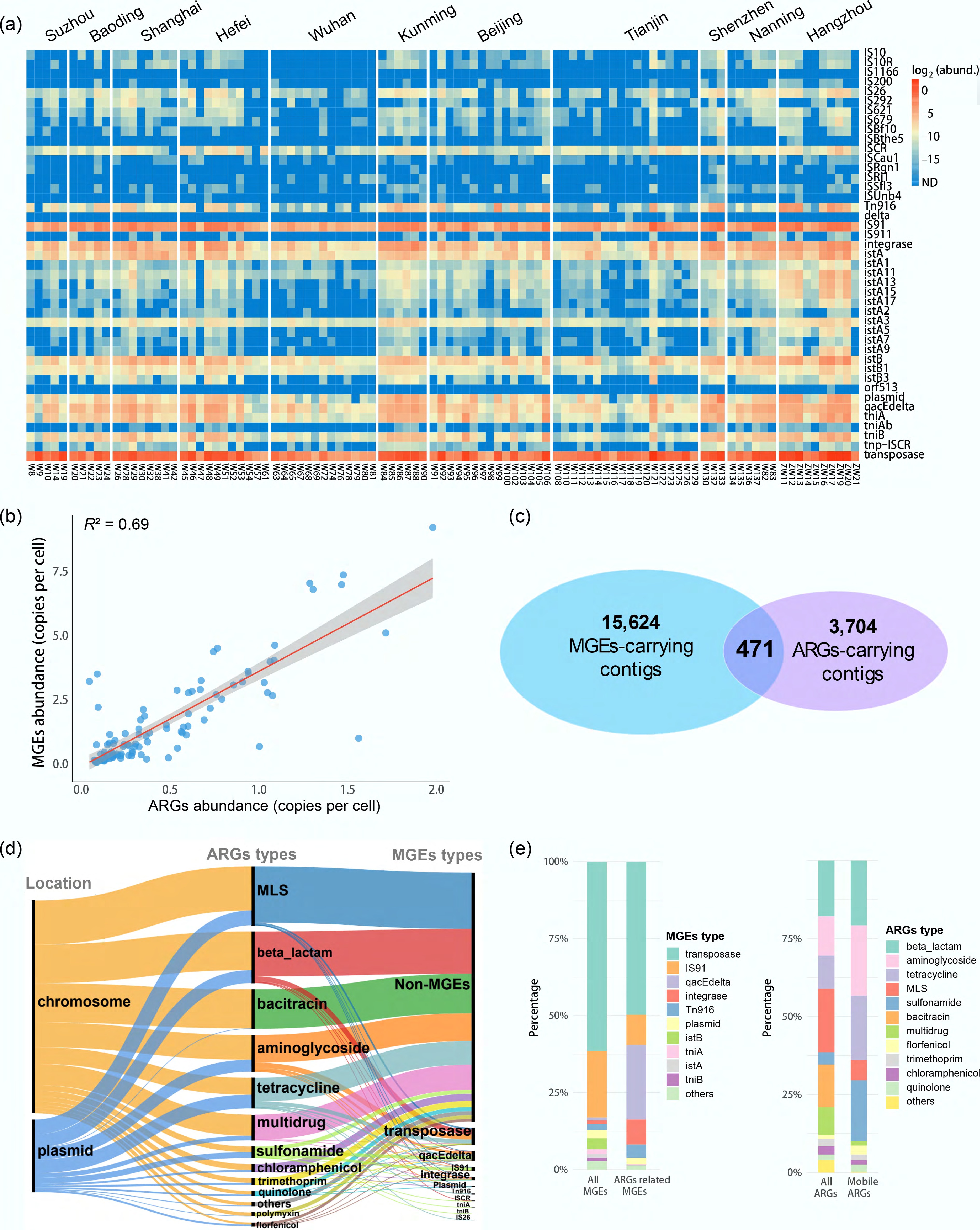
Figure 5.
MGEs profiles and their co-occurrence with ARGs. (a) MGEs' abundance across all samples. Abundance is displayed as log2-transformed copies per cell, with an offset of 1/10 of the minimum non-zero value added to each measurement to permit log transformation. (b) Linear correlation between the abundance (copies per cell) of ARGs and MGEs. (c) Venn diagram showing the number of contigs carrying MGEs, ARGs, or both. (d) Sankey diagram showing the distribution of contigs by their origin (chromosomes and plasmids), carried ARG types, and carried MGE types. (e) Composition of MGEs on all contigs vs on ARG-carrying contigs (left), and composition of ARGs on all contigs vs on MGEs-carrying contigs (right). The top 10 types are labeled; the remainder are grouped as 'others'.
-
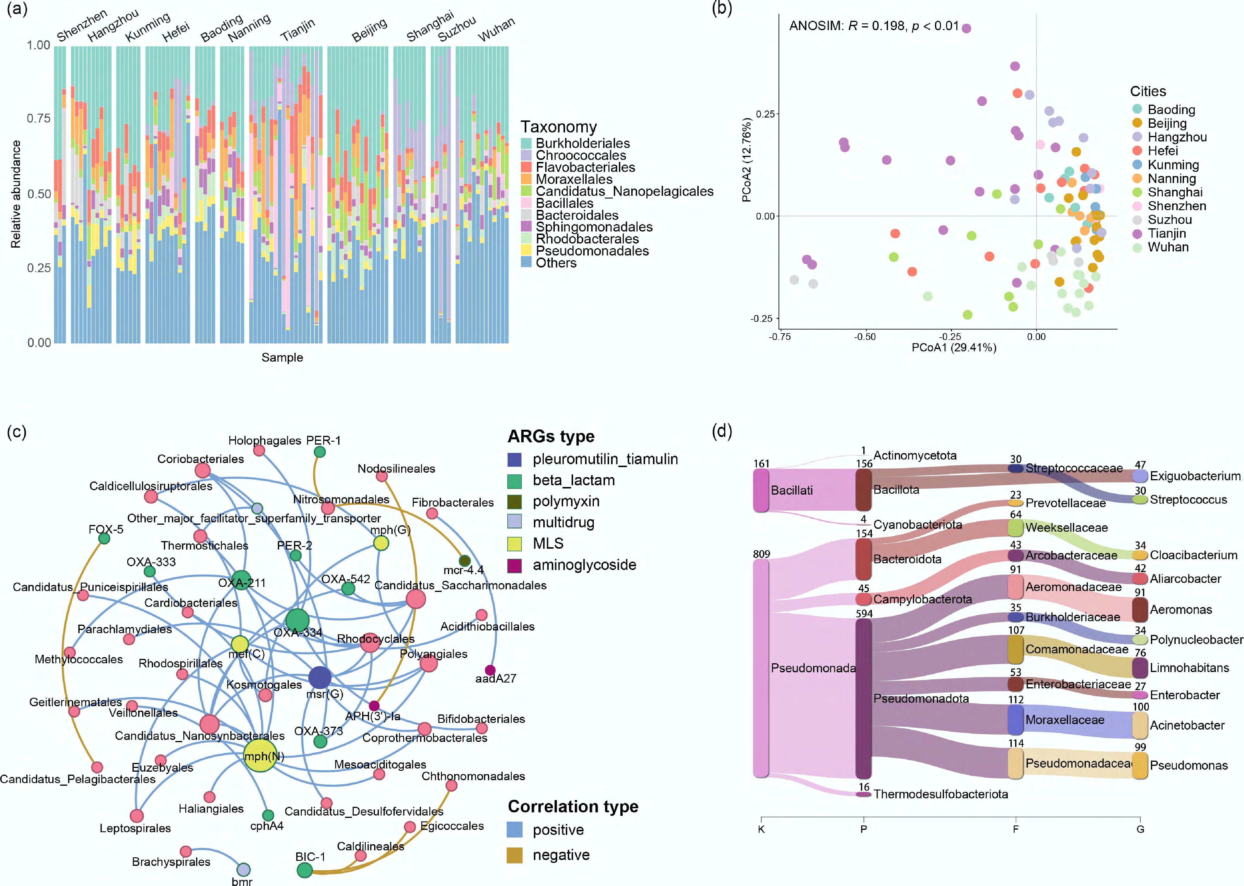
Figure 6.
Microbial community profiles and potential ARG hosts across sampling sites. (a) Relative abundance of the microbial community at the order level. The top 10 groups are labeled; the rest are grouped as 'Others'. (b) PCoA of the microbial community profile based on Bray–Curtis dissimilarity. (c) Co-occurrence network of ARGs and their potential hosts at the order level (Spearman's ρ > 0.4, p < 0.05). (d) Sankey diagram showing the host taxonomy of ARG-carrying contigs, with taxonomy names and contig numbers labeled on the bars.
Figures
(6)
Tables
(0)