Modeling and decoupling analysis for an integrated coupler and its non-compensated wireless power transfer system

Xueying Wu; He Li; Haisheng Wang; Xiaodong Qing; Qichang Feng; Zhengmei Lu; Xueying Wu; He Li; Haisheng Wang; Xiaodong Qing; Qichang Feng; Zhengmei Lu

doi:10.48130/wpt-0026-0007

Figures (23) Tables (7)

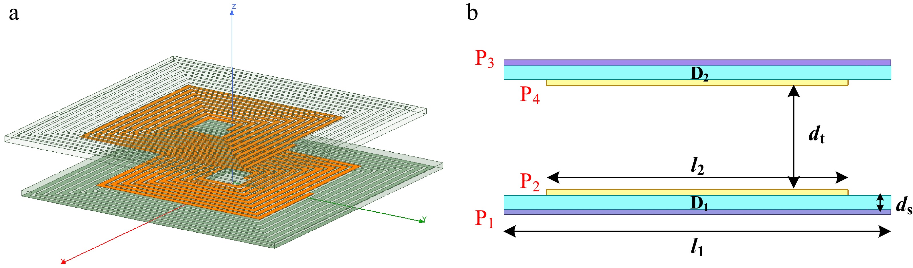
Figure 1.
Basic structure of the copper-foil electromagnetic coupler. (a) 3D graph of the coupler. (b) Front view^[22].
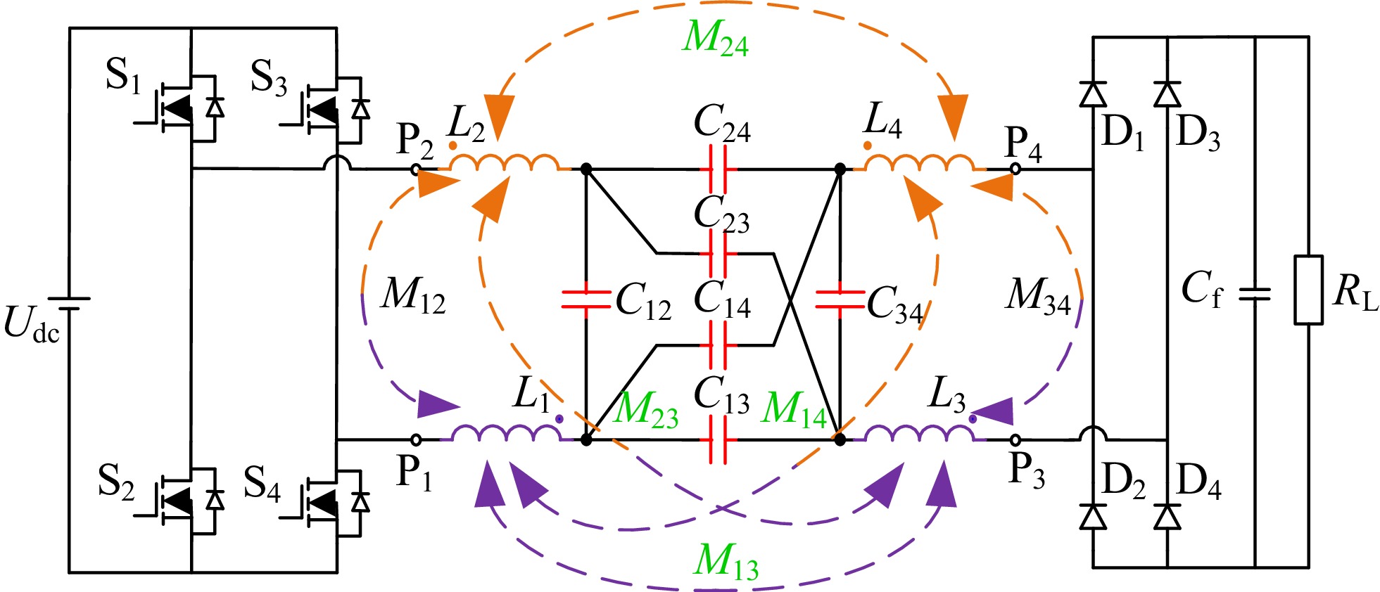
Figure 2.
Circuit topology of WPT system without compensation.
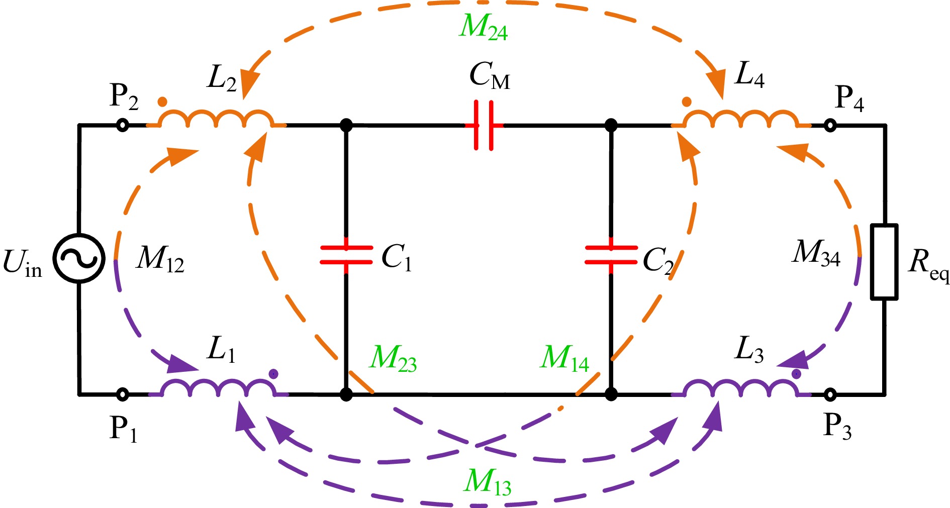
Figure 3.
System π-type equivalent model.
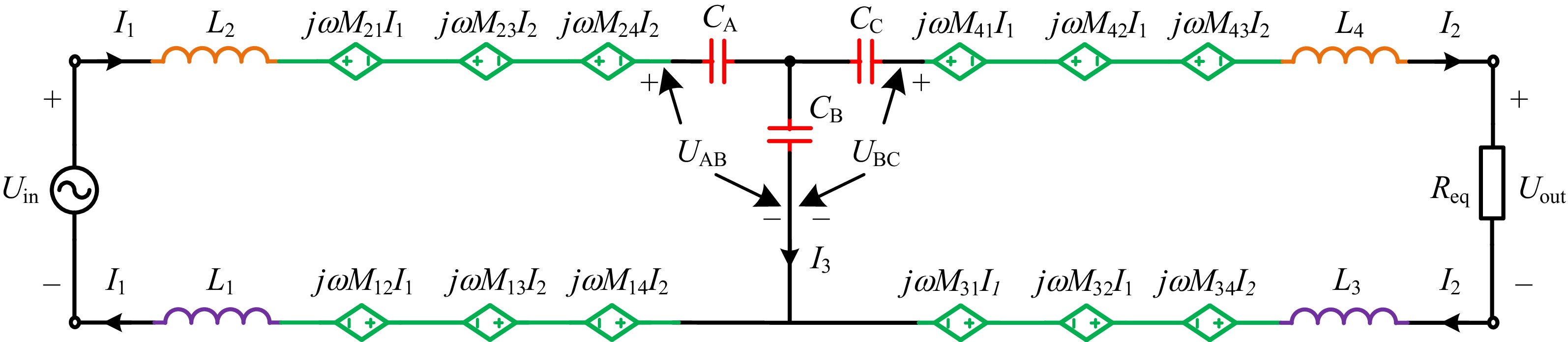
Figure 4.
Controlled source equivalent circuit.
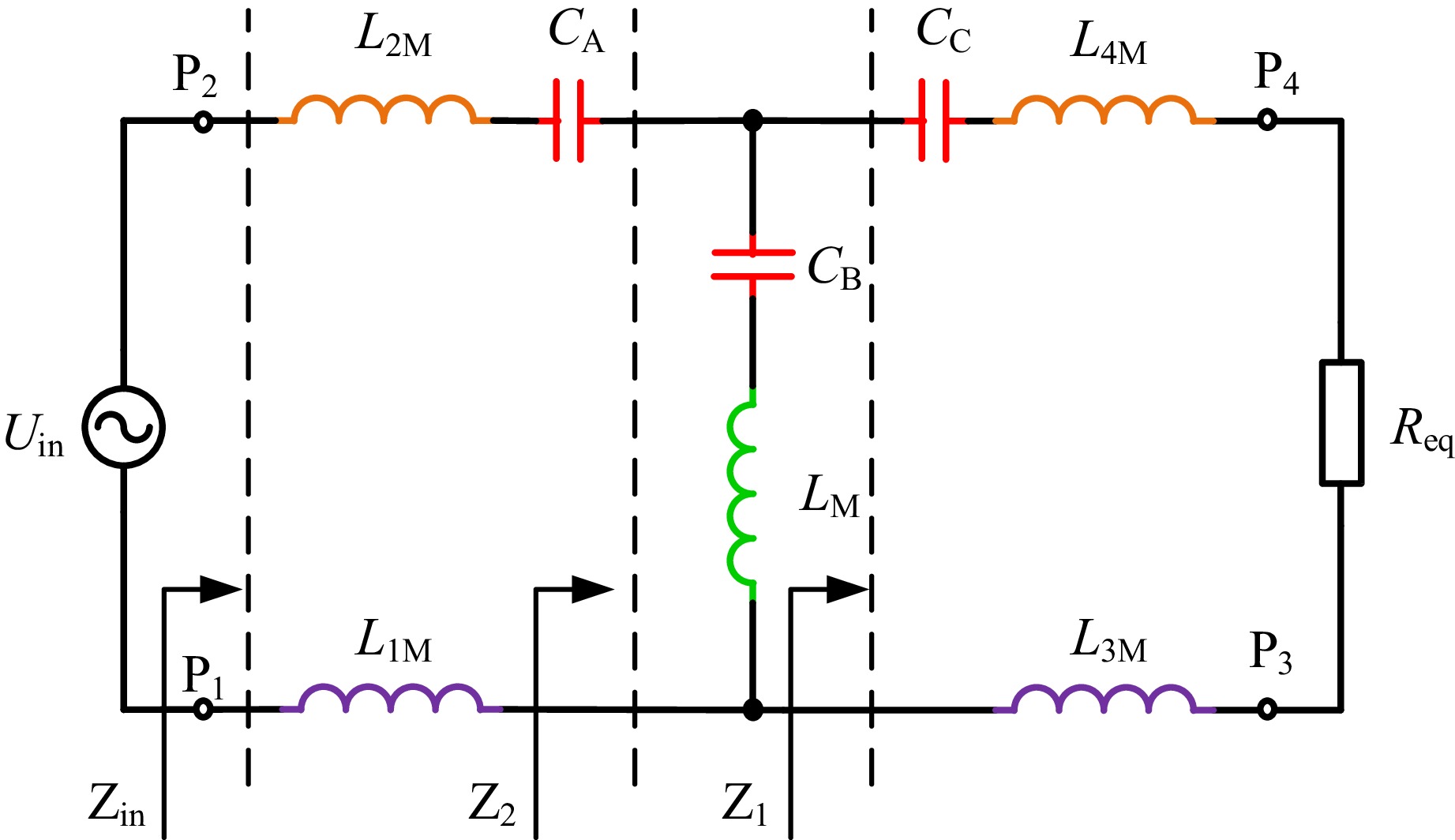
Figure 5.
System T-type decoupled model.
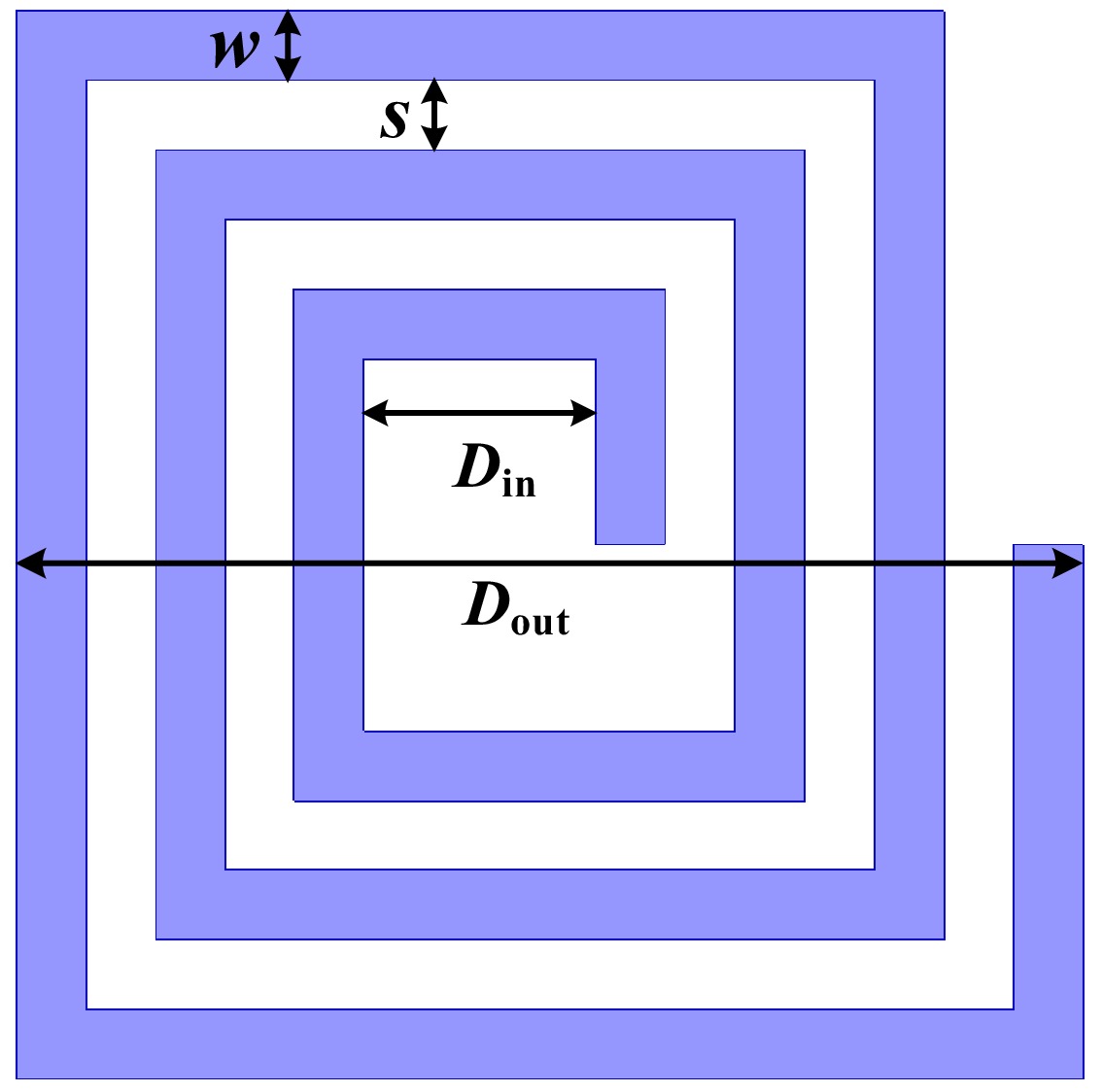
Figure 6.
Top view of the single coil.
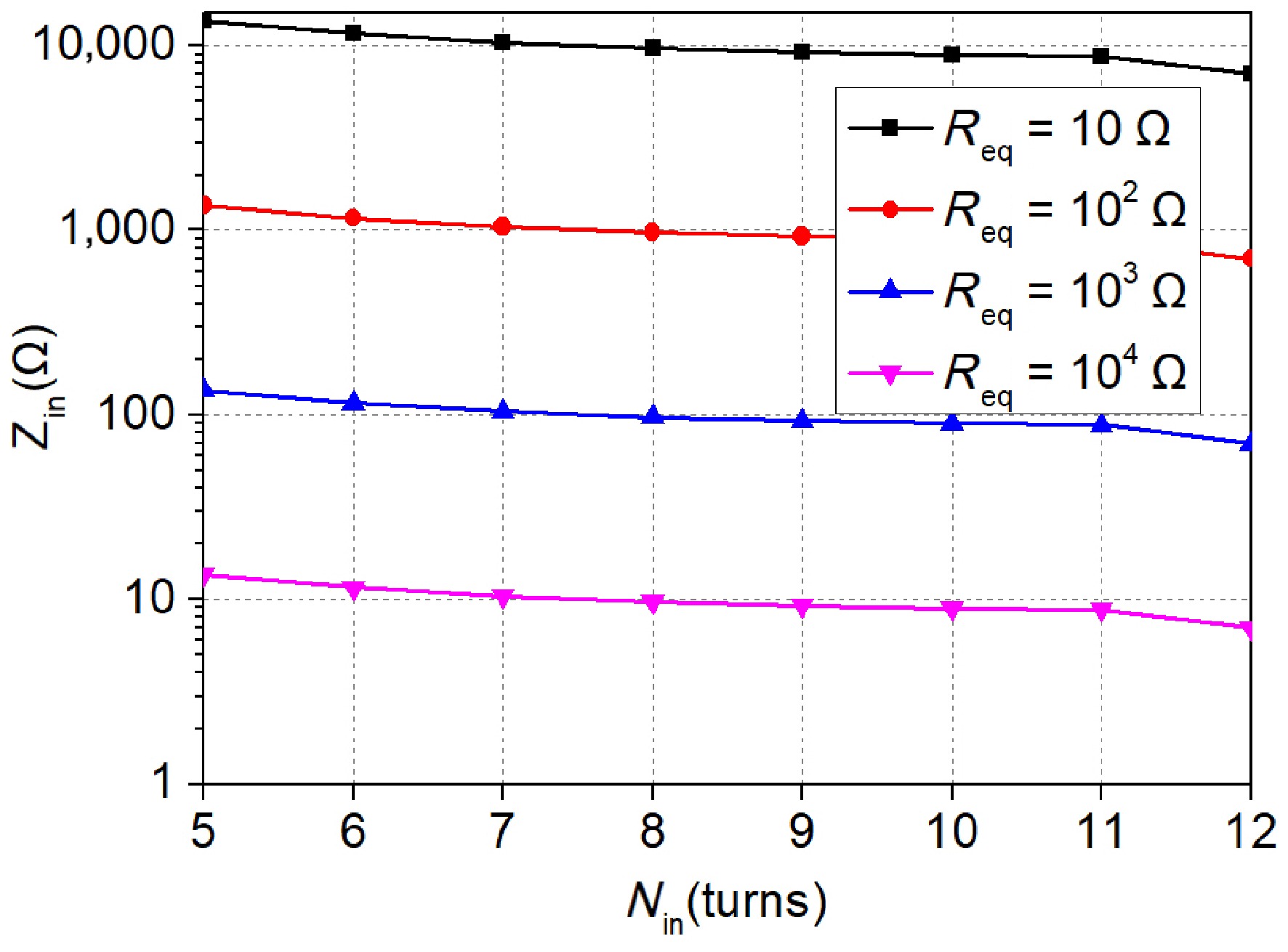
Figure 7.
Variation of the input impedance with N_inand R_eq^[22].
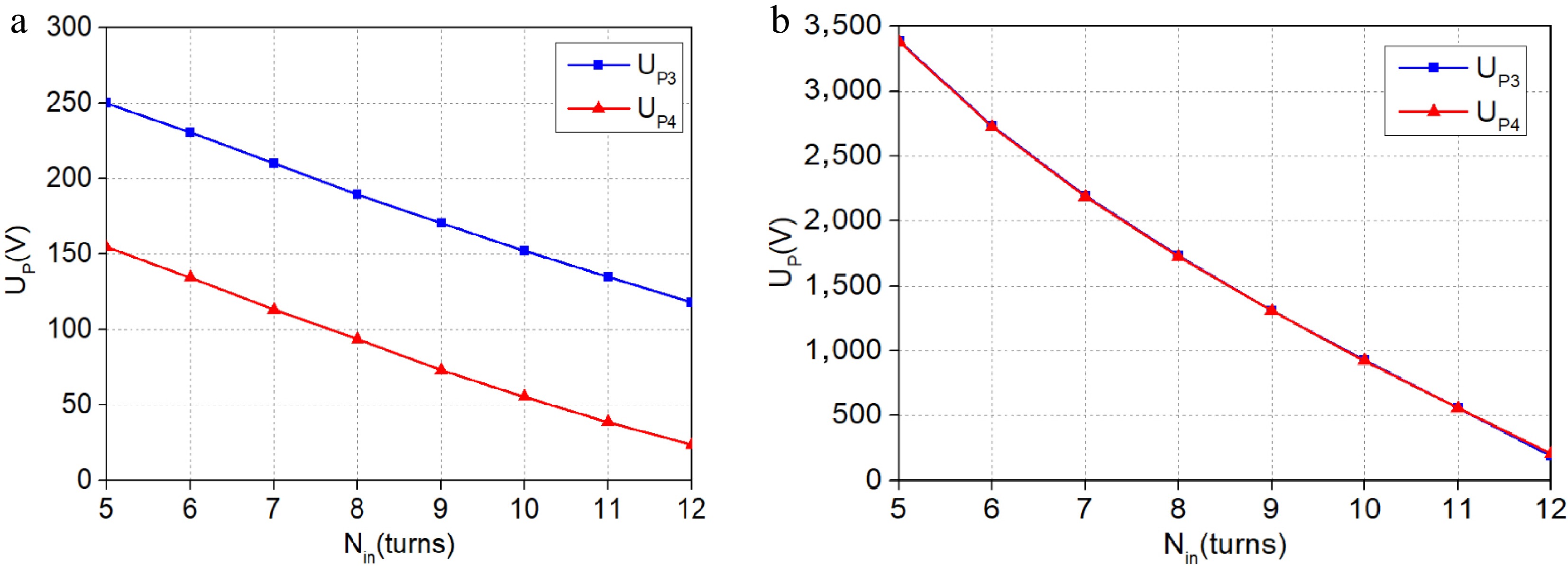
Figure 8.
Ground-referenced voltage curve of P₃ and P₄^[22]. (a) f = f₁. (b) f = f₂.
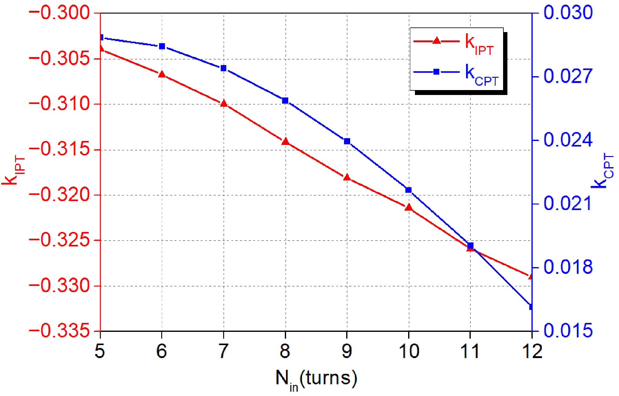
Figure 9.
Variation of magnetic-field and electric-field coupling coefficient.
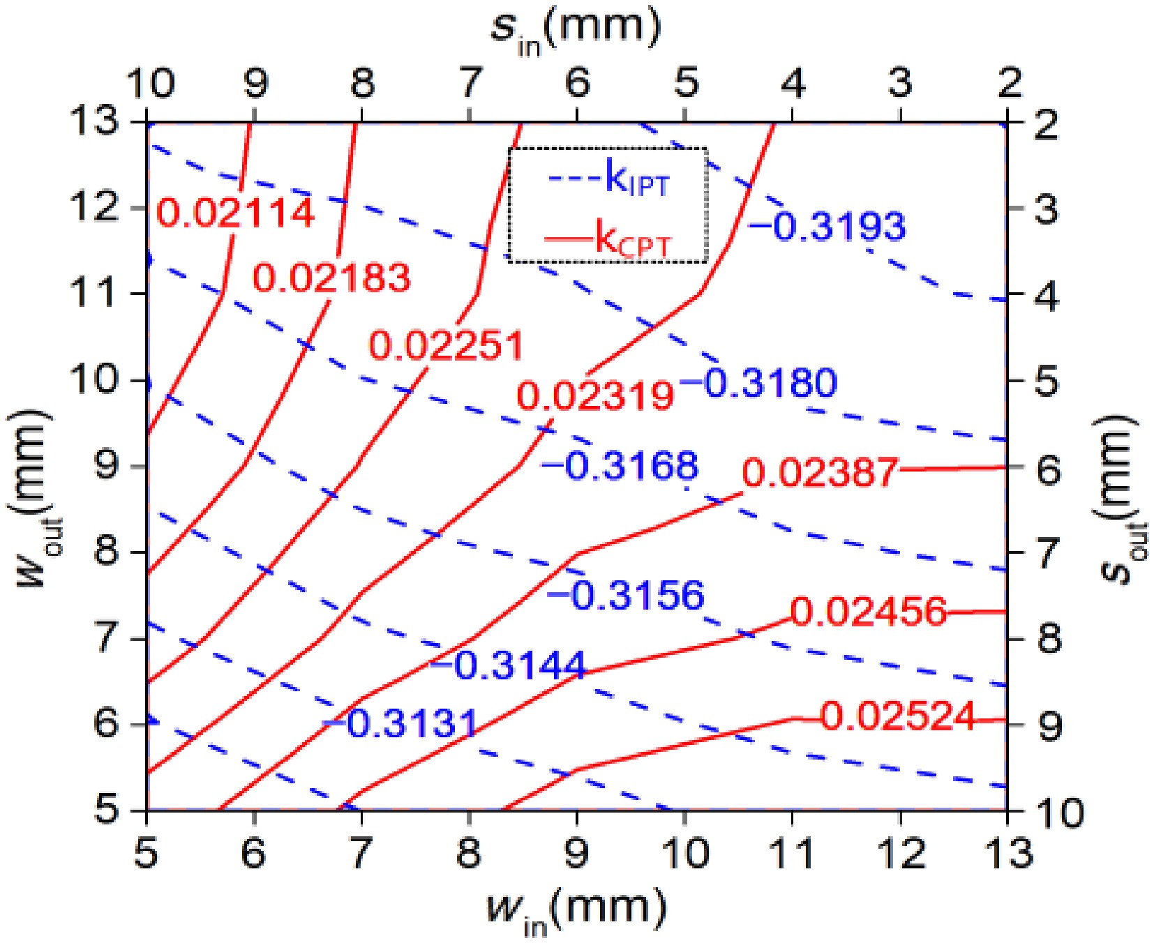
Figure 10.
The variation of coupling coefficient with w_in and w_out (or s_in and s_out).
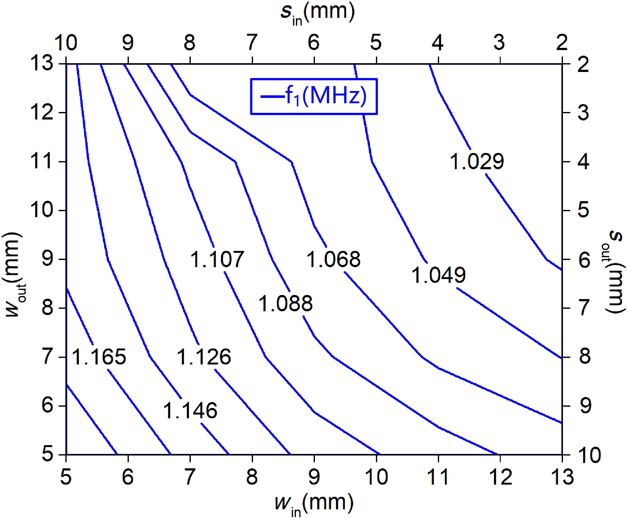
Figure 11.
The variation of the system resonance frequency f₁ with w_in and w_out (or s_in and s_out).
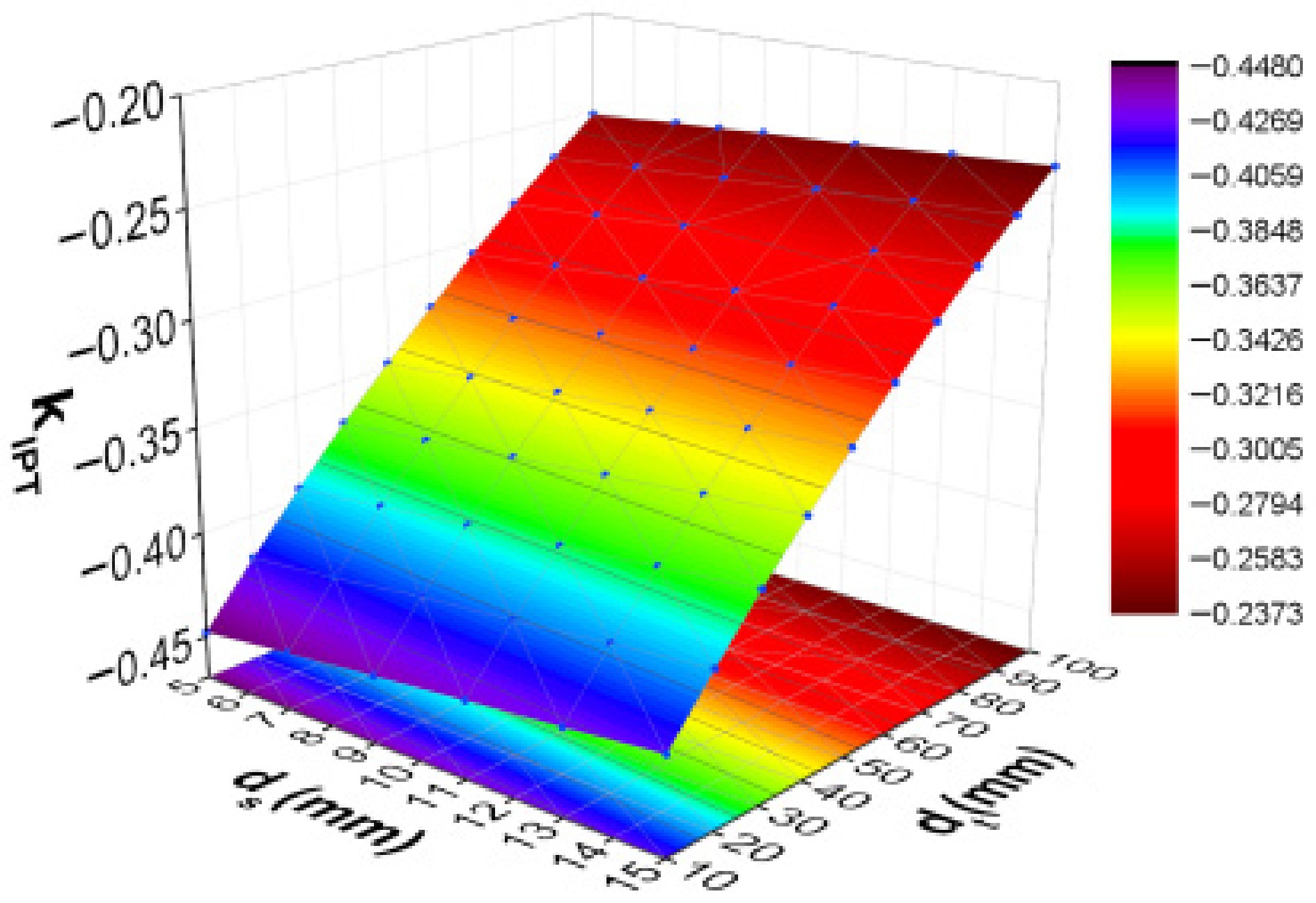
Figure 12.
The variation of k_IPT with d_s and d_t.
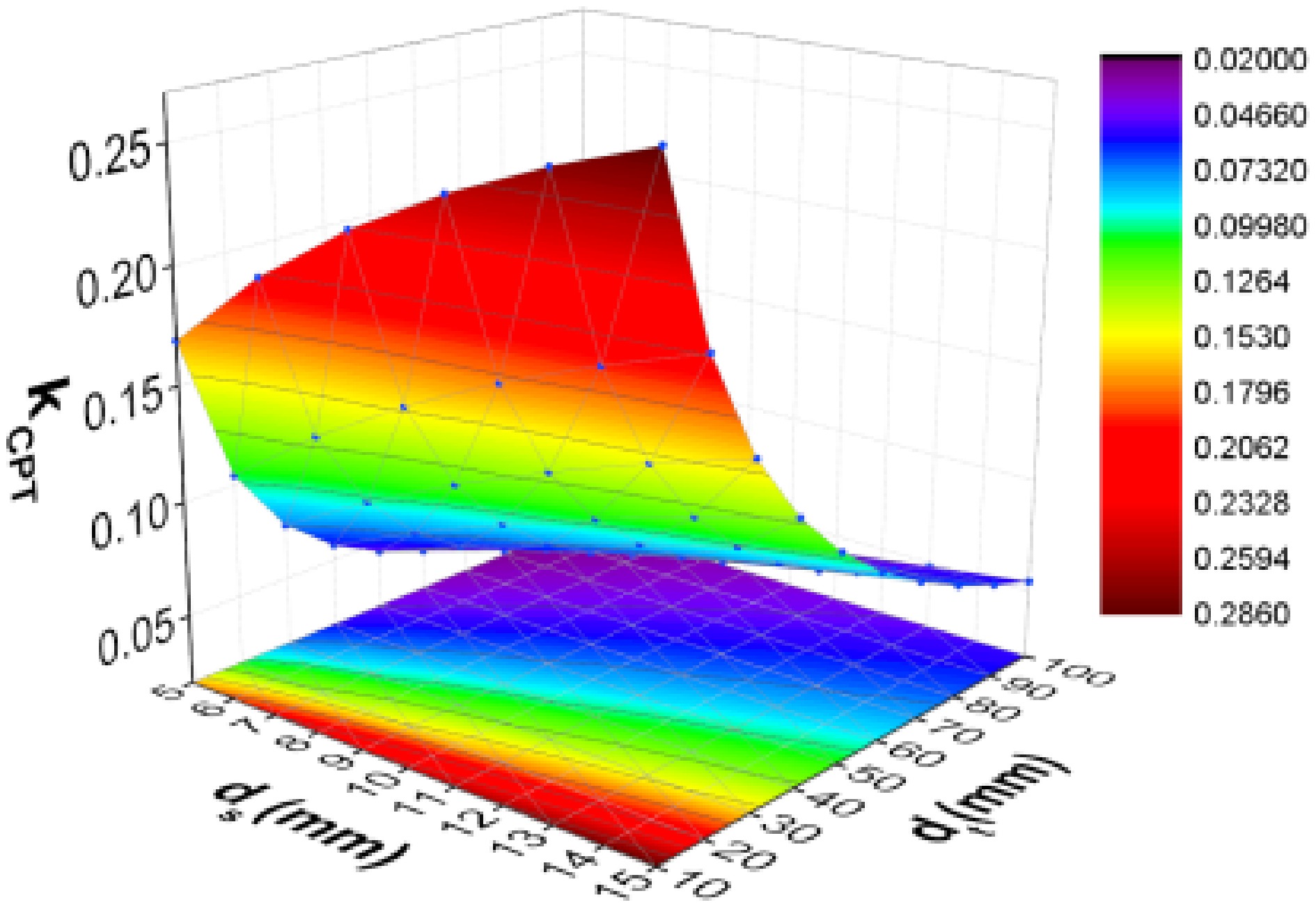
Figure 13.
The variation of k_CPT with d_s and d_t.
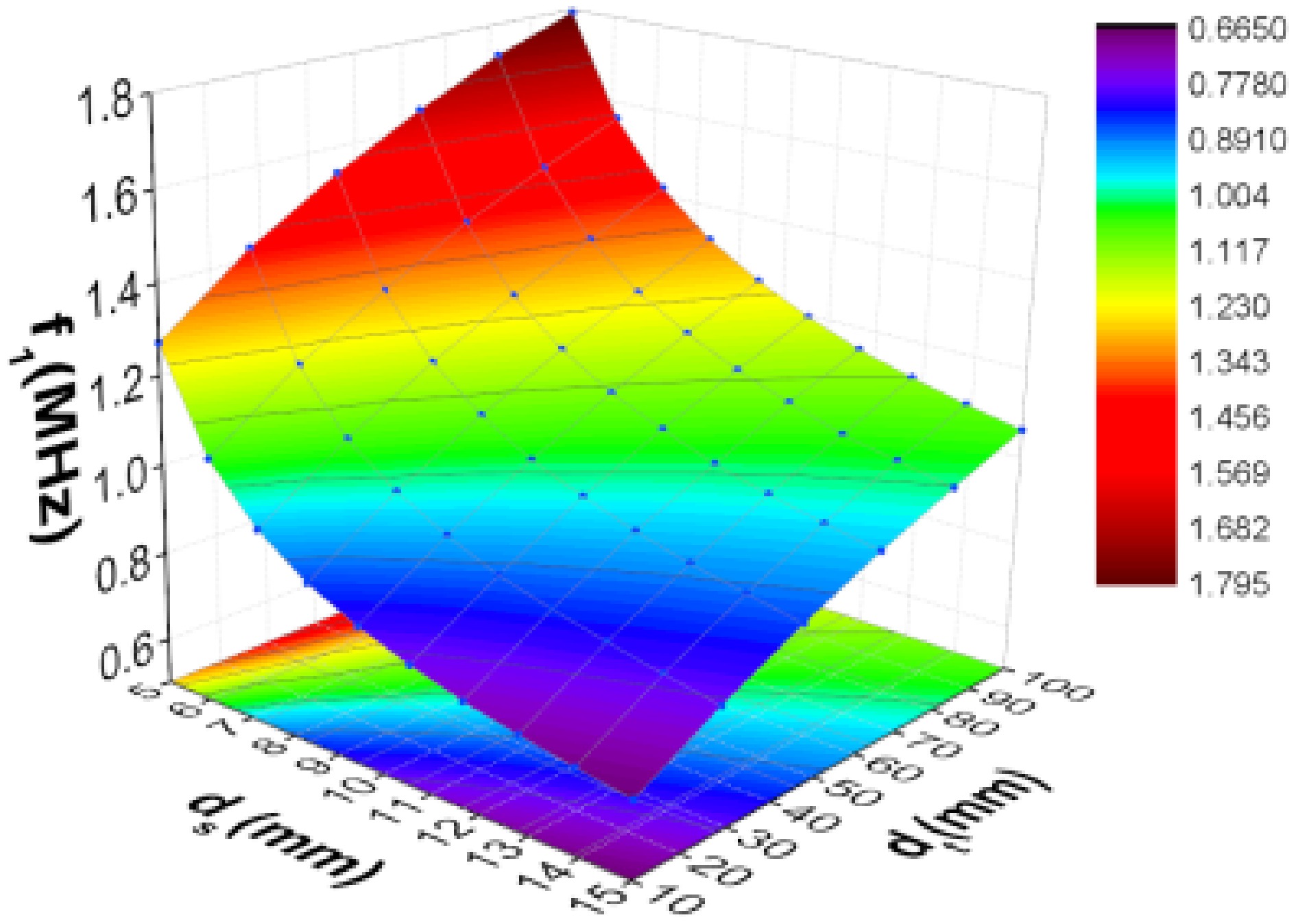
Figure 14.
The variation of f₁ with d_s and d_t.
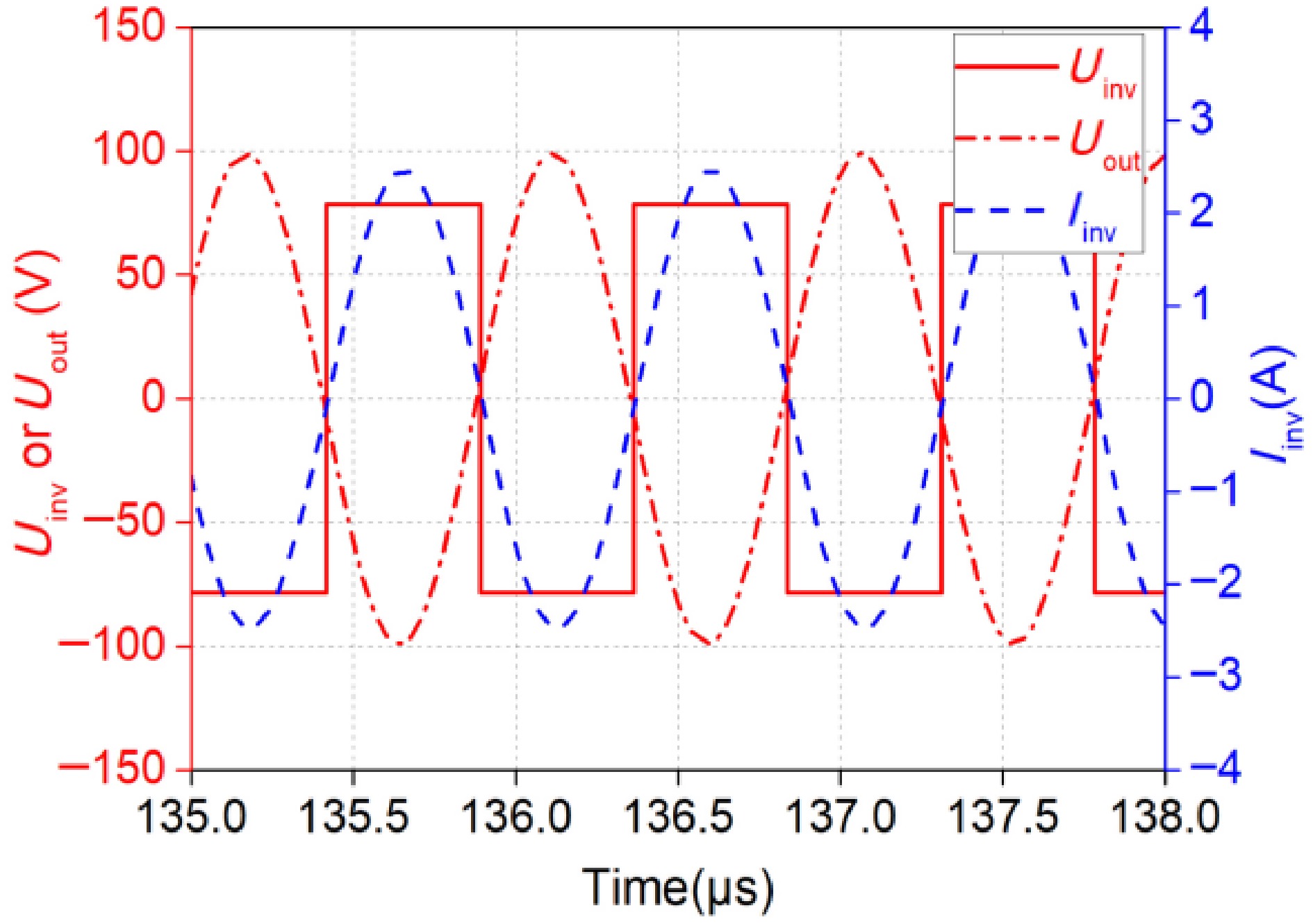
Figure 15.
Simulation waveforms of inverter output voltage and current.
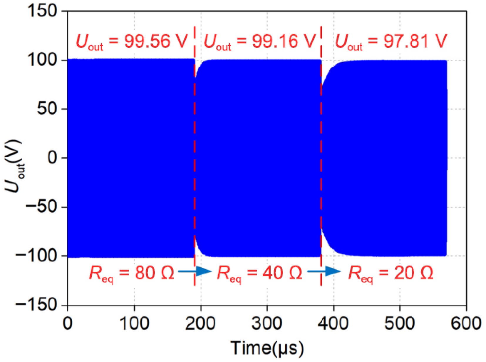
Figure 16.
Simulation waveforms of system output voltage varying with R_eq.
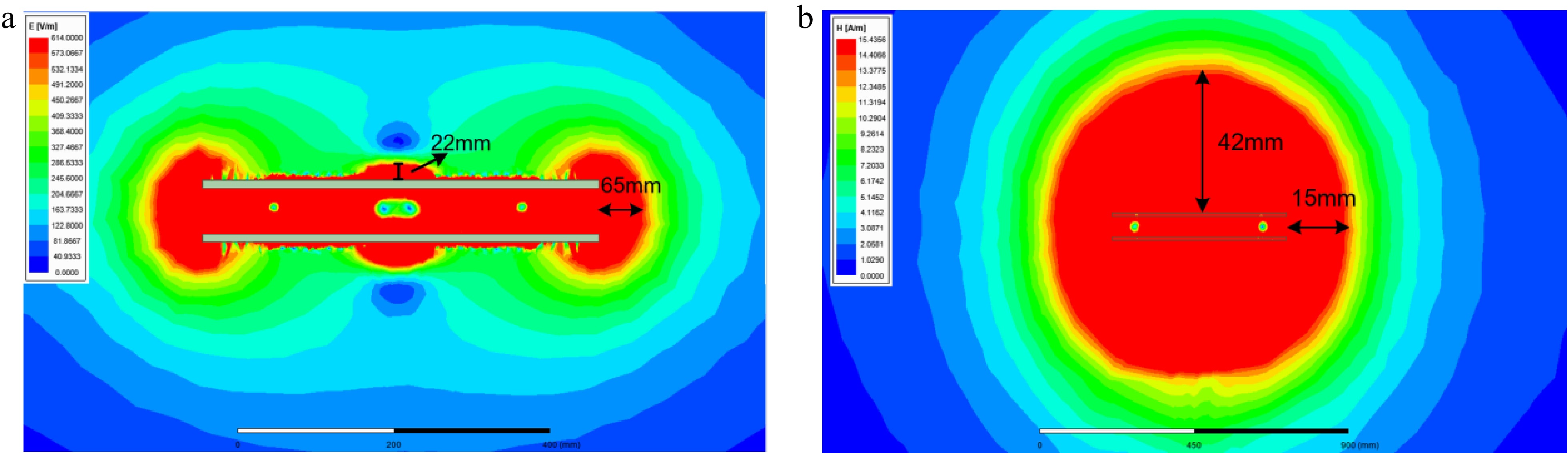
Figure 17.
(a) Electric field distribution around the coupler. (b) Magnetic field distribution around the coupler.
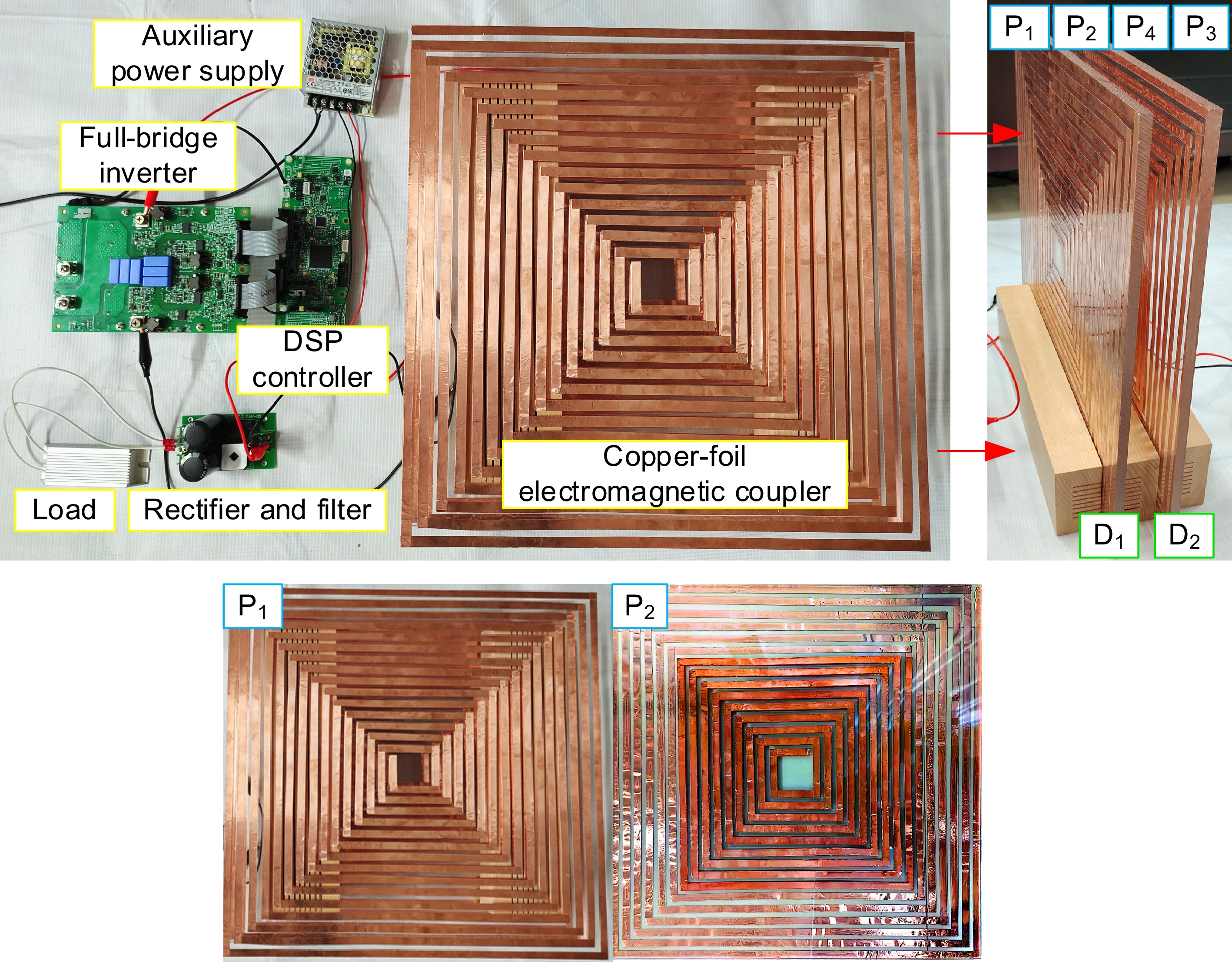
Figure 18.
Experimental prototype of the WPT system.
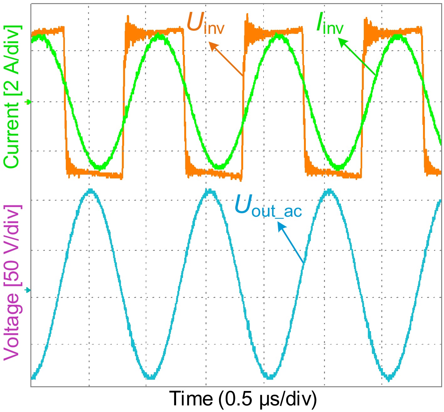
Figure 19.
Experimental waveforms of the inverter output and the AC load voltage.
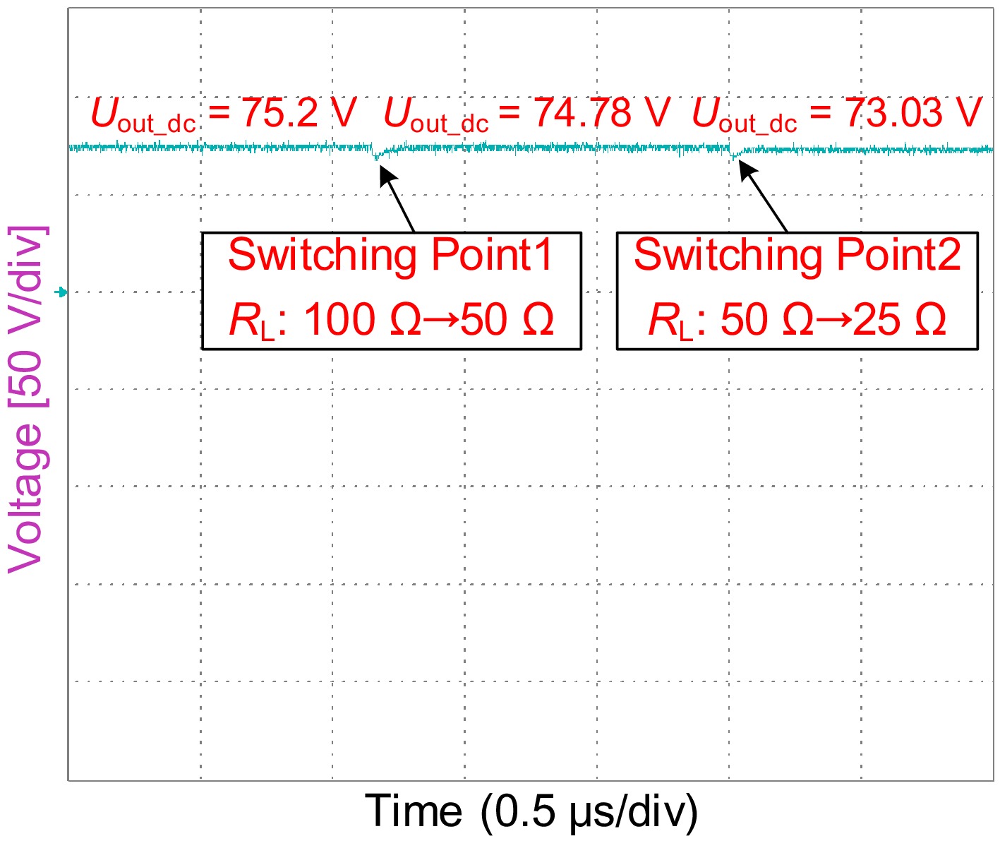
Figure 20.
Experimental waveforms of the DC load voltage when R_L changes (100→50→25 Ω).
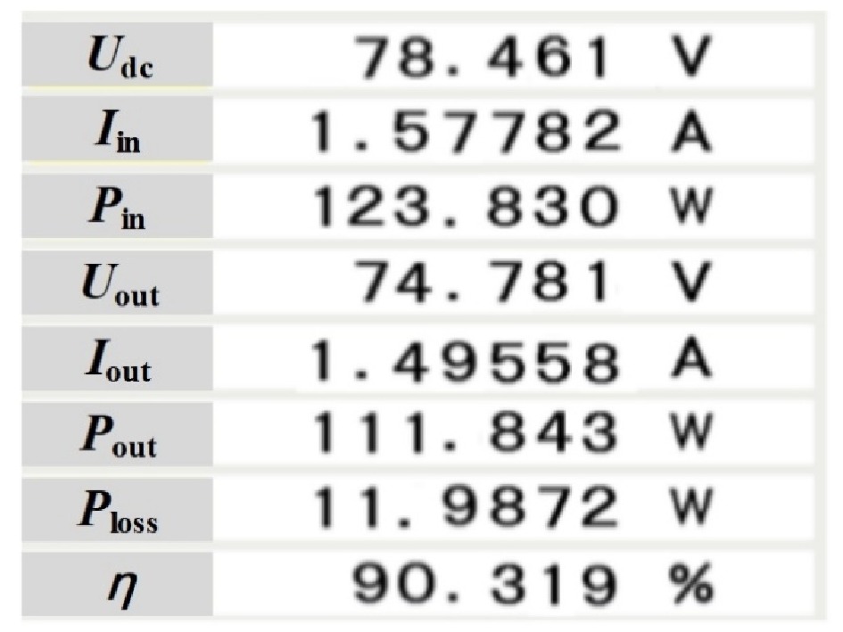
Figure 21.
The experiment results shown in power analyzer.
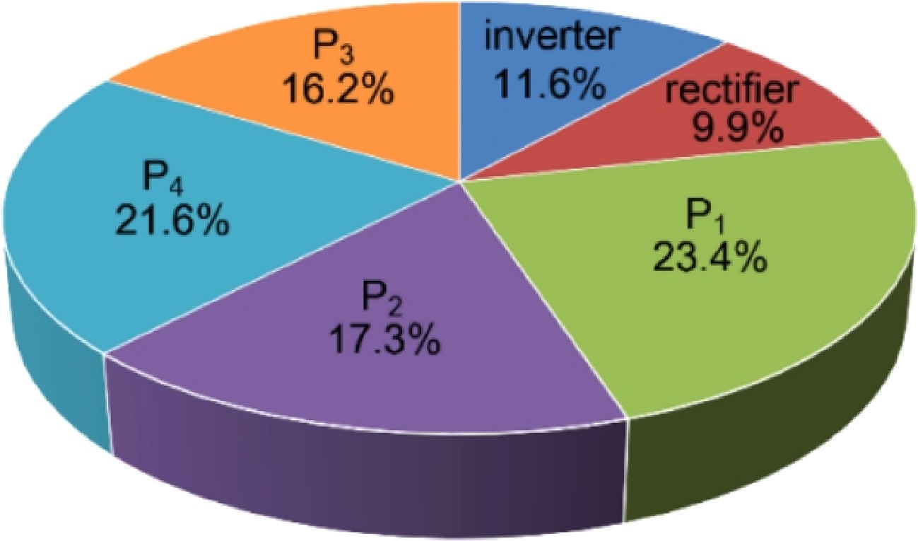
Figure 22.
Loss distributions of the experimental prototype.
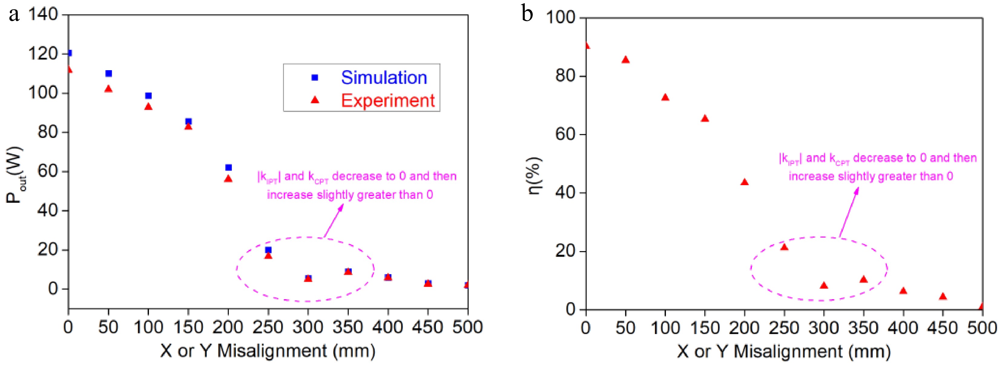
Figure 23.
(a) Test output power of the misalignment ability for this WPT system. (b) Experimental efficiency of the misalignment ability for this WPT system.

System parameters	First ZPA condition	Second ZPA condition
Operating angular frequency	$ \omega \text{=}\sqrt{\dfrac{{C}_{\text{A}}\text{+}{C}_{\text{B}}}{\left({L}_{1\text{M}}\text{+}{L}_{\text{2M}}\text{+}{L}_{\text{M}}\right){C}_{\text{A}}{C}_{\text{B}}}} $	$ \begin{cases} {\omega }_{1}\text{=}\sqrt{\dfrac{-B+\sqrt{{B}^{2}-4AC}}{2A}}\\{\omega }_{2}\text{=}\sqrt{\dfrac{-B-\sqrt{{B}^{2}-4AC}}{2A}}\end{cases} $
Input impedance	$ {Z}_{\text{in}}\text{=}\dfrac{{\left(\left({L}_{1\text{M}}\text{+}{L}_{\text{2M}}\right){C}_{\text{A}}-{L}_{\text{M}}{C}_{\text{B}}\right)}^{2}}{\left({L}_{\text{M}}+{L}_{1\text{M}}\text{+}{L}_{\text{2M}}\right)\left({C}_{\text{A}}+{C}_{\text{B}}\right){C}_{\text{A}}{C}_{\text{B}}{R}_{\text{eq}}} $	$ {R}_{\text{eq}} $
Output voltage	$ {\dot{U}}_{\text{out}}=-j{\dot{U}}_{\text{in}}{R}_{\text{eq}}\dfrac{\sqrt{\left({L}_{\text{M}}+{L}_{1\text{M}}\text{+}{L}_{\text{2M}}\right)\left({C}_{\text{A}}+{C}_{\text{B}}\right){C}_{\text{A}}{C}_{\text{B}}}}{\left({L}_{1\text{M}}\text{+}{L}_{\text{2M}}\right){C}_{\text{A}}-{L}_{\text{M}}{C}_{\text{B}}} $	$ {\dot{U}}_{\text{out}}=-{\dot{U}}_{\text{in}}\cdot \dfrac{{\omega }^{2}{C}_{\text{A}}\left({L}_{1\text{M}}\text{+}{L}_{\text{2M}}\right)-1\text{+}j\omega {C}_{\text{A}}{R}_{\text{eq}}}{{\omega }^{2}{C}_{\text{A}}\left({L}_{1\text{M}}\text{+}{L}_{\text{2M}}\right)-1-j\omega {C}_{\text{A}}{R}_{\text{eq}}} $
Output current	$ {\dot{I}}_{\text{out}}=-j\dfrac{\sqrt{\left({L}_{\text{M}}+{L}_{1\text{M}}\text{+}{L}_{\text{2M}}\right)\left({C}_{\text{A}}+{C}_{\text{B}}\right){C}_{\text{A}}{C}_{\text{B}}}}{\left({L}_{1\text{M}}\text{+}{L}_{\text{2M}}\right){C}_{\text{A}}-{L}_{\text{M}}{C}_{\text{B}}} {\dot{U}}_{\text{in}}$	$ {\dot{I}}_{\text{out}}=-\dfrac{{\dot{U}}_{\text{in}}}{{R}_{\text{eq}}}\dfrac{{\omega }^{2}{C}_{\text{A}}\left({L}_{1\text{M}}\text{+}{L}_{\text{2M}}\right)-1\text{+}j\omega {C}_{\text{A}}{R}_{\text{eq}}}{{\omega }^{2}{C}_{\text{A}}\left({L}_{1\text{M}}\text{+}{L}_{\text{2M}}\right)-1-j\omega {C}_{\text{A}}{R}_{\text{eq}}} $

Table 1.

System parameters in two ZPA conditions.

Parameter Value Parameter Value

N_out 15 d_t 60 mm
s_out 5 mm s_in 5 mm
d_s 10 mm w_out 10 mm
w_in 10 mm

Table 2.
Parameters of the coupler when Nin is variable.
Parameter Value Parameter Value

N_out 15 N_in 9

s_out + w_out 15 mm d_t 60 mm

d_s 10 mm s_in + w_in 15 mm

Table 3.
Parameters of the coupler when sout and wout are variable.
Parameter Value Parameter Value

N_out 15 N_in 9

s_out 5 mm s_in 5 mm

w_out 10 mm w_in 10 mm

R_eq 40 Ω

Table 4.
Parameters of the coupler when d_s and d_t are variable.
Parameter Value Parameter Value

N_out 15 N_in 9
s_out 5 mm s_in 5 mm
w_out 10 mm w_in 10 mm
d_s 10 mm d_t 60 mm

Table 5.
Geometric parameters of the coupler.

Parameter	Value	Parameter	Value	Parameter	Value
f	1.056 MHz	M₁₂	22.731μH	C₁₂	324.98 pF
U_dc (U_in)	78.54V (100 V)	M₁₃	28.369 μH	C₁₃	30.376 pF
R_L (R_eq)	49.348 Ω (40 Ω)	M₁₄	12.367 μH	C₁₄	3.0998 pF
L₁	64.622 μH	M₂₃	12.366 μH	C₂₃	3.1395 pF
L₂	19.517 μH	M₂₄	7.2848 μH	C₂₄	13.198 pF
L₃	64.407 μH	M₃₄	22.722 μH	C₃₄	324.14 pF
L₄	19.432 μH

Table 6.

Circuit parameters for simulation.

Parameter Value Parameter Value

U_P1-G 100 V U_P2-G 100 V
U_P3-G 170.9 V U_P4-G 72.24 V
I_P1 2.484 A I_P2 2.484 A
I_P3 2.475 A I_P4 2.475 A

Table 7.
Amplitude value of the voltage to ground and current of P₁−P₄.

Parameter	Value	Parameter	Value
N_out	15	d_t	60 mm
s_out	5 mm	s_in	5 mm
d_s	10 mm	w_out	10 mm
w_in	10 mm

Parameter	Value	Parameter	Value
N_out	15	N_in	9
s_out + w_out	15 mm	d_t	60 mm
d_s	10 mm	s_in + w_in	15 mm

Parameter	Value	Parameter	Value
N_out	15	N_in	9
s_out	5 mm	s_in	5 mm
w_out	10 mm	w_in	10 mm
R_eq	40 Ω

Parameter	Value	Parameter	Value
N_out	15	N_in	9
s_out	5 mm	s_in	5 mm
w_out	10 mm	w_in	10 mm
d_s	10 mm	d_t	60 mm