Back Article

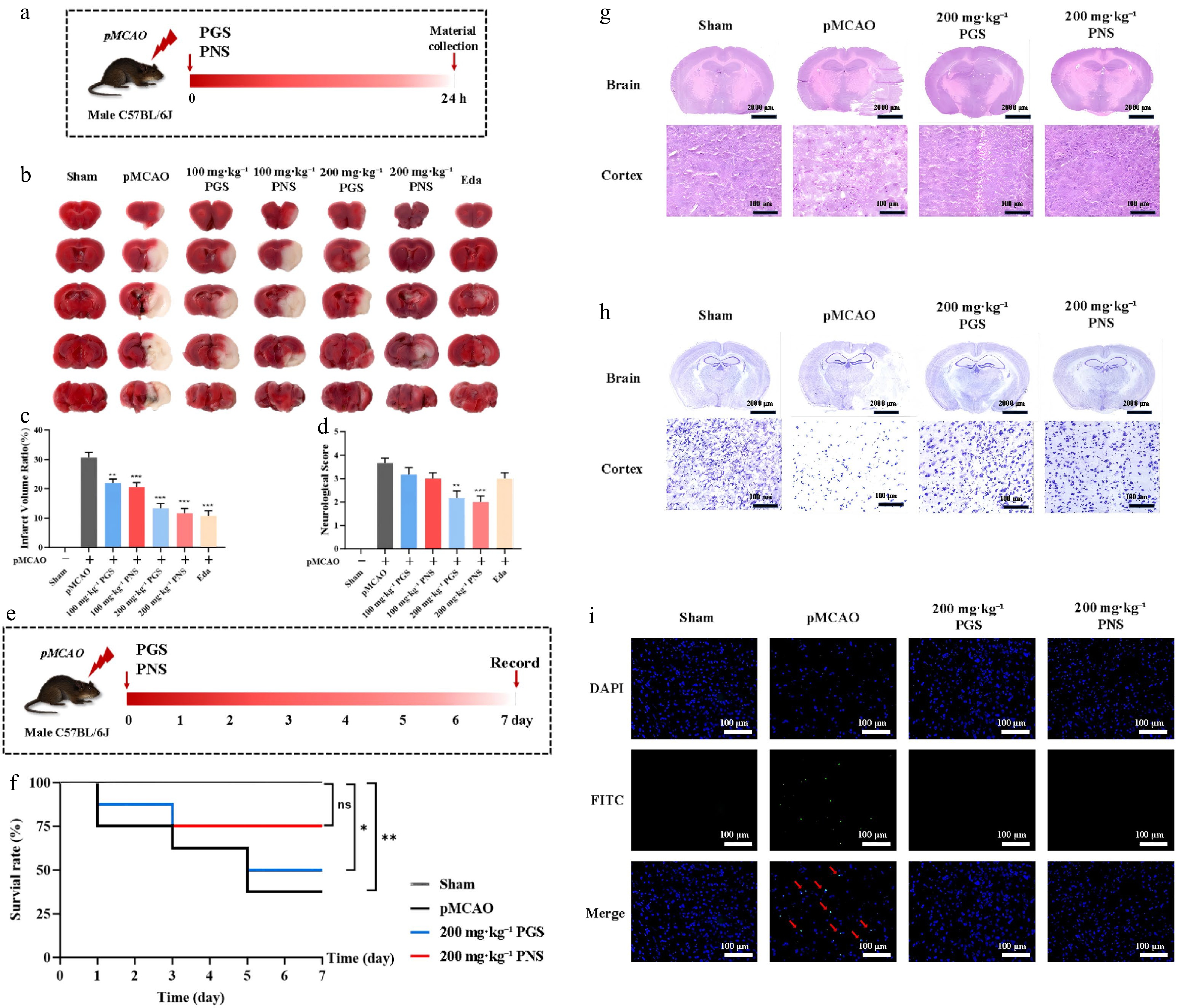
Figure 1. 

PNS and PGS alleviate acute cerebral ischemic injury in pMCAO mice. (a) Experimental design of the pMCAO model and drug administration. Mice were subjected to pMCAO followed by intragastric administration of vehicle, PNS (100 mg·kg⁻¹ and 200 mg·kg⁻¹), and PGS (100 mg·kg⁻¹ and 200 mg·kg⁻¹) immediately after surgery. Neurological function was evaluated after 24 h, followed by tissue collection for TTC staining, histological examination, and molecular analyses. (b) Representative TTC-stained coronal brain sections showing cerebral infarct areas in Sham, pMCAO, PNS, and PGS groups. The white region indicates infarcted tissue, whereas the red region represents viable brain tissue. (c) Quantification of cerebral infarct volume calculated from TTC-stained sections. (d) Neurological scores assessed 24 h after pMCAO. (e) Schematic diagram of the experimental design for the 7-d survival study. Mice were subjected to permanent middle cerebral artery occlusion and immediately treated with vehicle, PNS (200 mg·kg⁻¹), or PGS (200 mg·kg⁻¹) by oral gavage after surgery. Survival was monitored daily for seven consecutive days, and survival rates were recorded throughout the observation period. (f) Kaplan–Meier survival curves of mice following pMCAO. Survival was monitored for 7 d after surgery in the Sham, pMCAO, PNS, and PGS groups (n = 8 mice per group). Survival differences among groups were analyzed using the log-rank (Mantel–Cox) test. Data are presented as survival probability over time. Statistical significance was defined as P < 0.05. Compared with the pMCAO group, * P < 0.05 and ** P < 0.01. (g) Representative H&E staining of ischemic brain sections collected at 24 h after pMCAO (acute treatment experiment). Low-magnification images illustrate overall lesion morphology, whereas high-magnification images show neuronal architecture within the ischemic cortex. Scale bars: 2,000 μm (upper panels) and 100 μm (lower panels). (h) Representative Nissl staining of ischemic brain sections collected at 24 h after pMCAO (acute treatment experiment). Intact neurons containing abundant Nissl bodies appear dark blue-purple, whereas injured neurons exhibit reduced Nissl substance and disrupted cellular morphology. Scale bars: 2,000 μm (upper panels) and 100 μm (lower panels). (i) Representative immunofluorescence images of TUNEL staining performed on brain sections collected at 24 h after pMCAO (acute treatment experiment). Blue indicates DAPI-stained nuclei, green indicates TUNEL-positive apoptotic cells, and merged images illustrate the spatial distribution of apoptotic neurons. Red arrows indicate representative TUNEL-positive cells. Scale bar = 100 μm. (n = 3). Data are presented as mean ± SD, n = 6. Statistical analyses were performed using one-way analysis of variance (ANOVA) followed by Tukey's multiple-comparison test. Neurological deficit scores were analyzed using the Kruskal–Wallis test followed by Dunn's post hoc test because the data were non-normally distributed. Statistical significance was defined as P < 0.05; * P < 0.05; ** P < 0.01; *** P < 0.001 vs the pMCAO group.

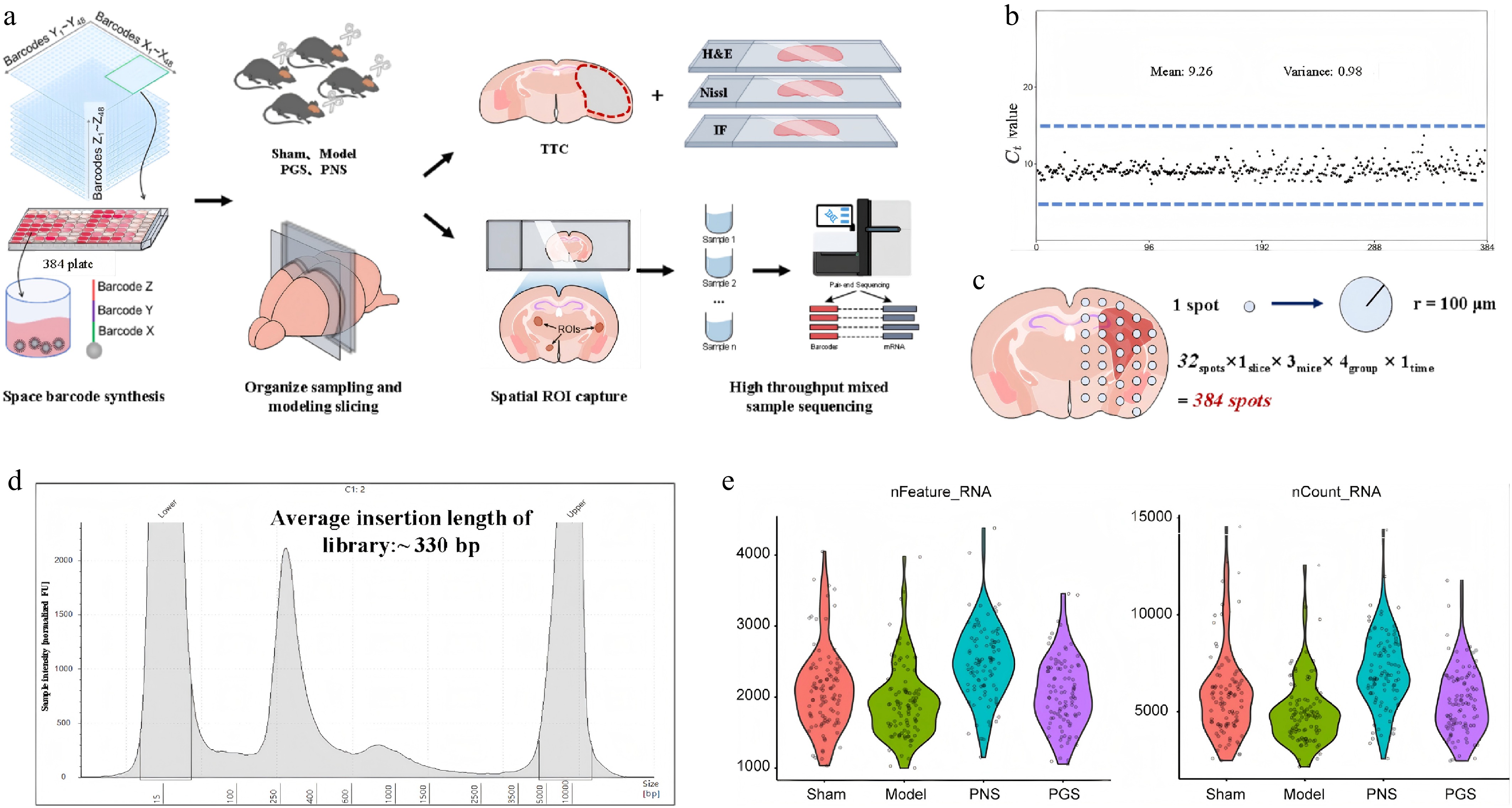
Figure 2. 

Overview of the Spatial-seq 2.0 workflow and quality control of spatial transcriptomic data. (a) Schematic illustration of the Spatial-seq 2.0 workflow. The experimental procedure includes spatial barcode synthesis, establishment of the pMCAO mouse model, cryosection preparation, LCM of spatial ROIs, mRNA capture by spatially barcoded magnetic beads, reverse transcription, cDNA library construction, high-throughput sequencing, and downstream bioinformatic analyses. Consecutive brain sections were collected for H&E staining and Nissl staining to facilitate spatial registration and histopathological validation. (b) Quality assessment of spatially barcoded magnetic beads. The C_t values obtained by qRT-PCR were used to evaluate the amplification efficiency and uniformity of all 384 uniquely barcoded magnetic beads. Each black dot represents one barcode, the solid horizontal line indicates the mean C_t value, and the blue dashed lines denote the acceptable quality-control range. The low variance demonstrates the high consistency of barcode synthesis and amplification efficiency. (c) Spatial distribution of captured spots. Spatial ROIs were collected from the ipsilateral hemisphere using LCM. A total of 384 spatial spots were obtained from four experimental groups (32 spots per section × 3 mice per group × 4 groups). Each spot had a radius of approximately 100 μm, corresponding to a localized tissue region for spatial transcriptomic analysis. (d) Sequencing library quality assessment. Representative electropherogram showing the fragment-size distribution of the cDNA library. The average insert size was approximately 330 bp, indicating that the library met the quality requirements for Illumina paired-end sequencing. (e) Quality control of spatial transcriptomic sequencing data. Violin plots show the distributions of the number of detected genes (nFeature_RNA) and total transcript counts (nCount_RNA) across all spatial spots in the Sham, pMCAO, PNS, and PGS groups. Each dot represents one spatial spot.

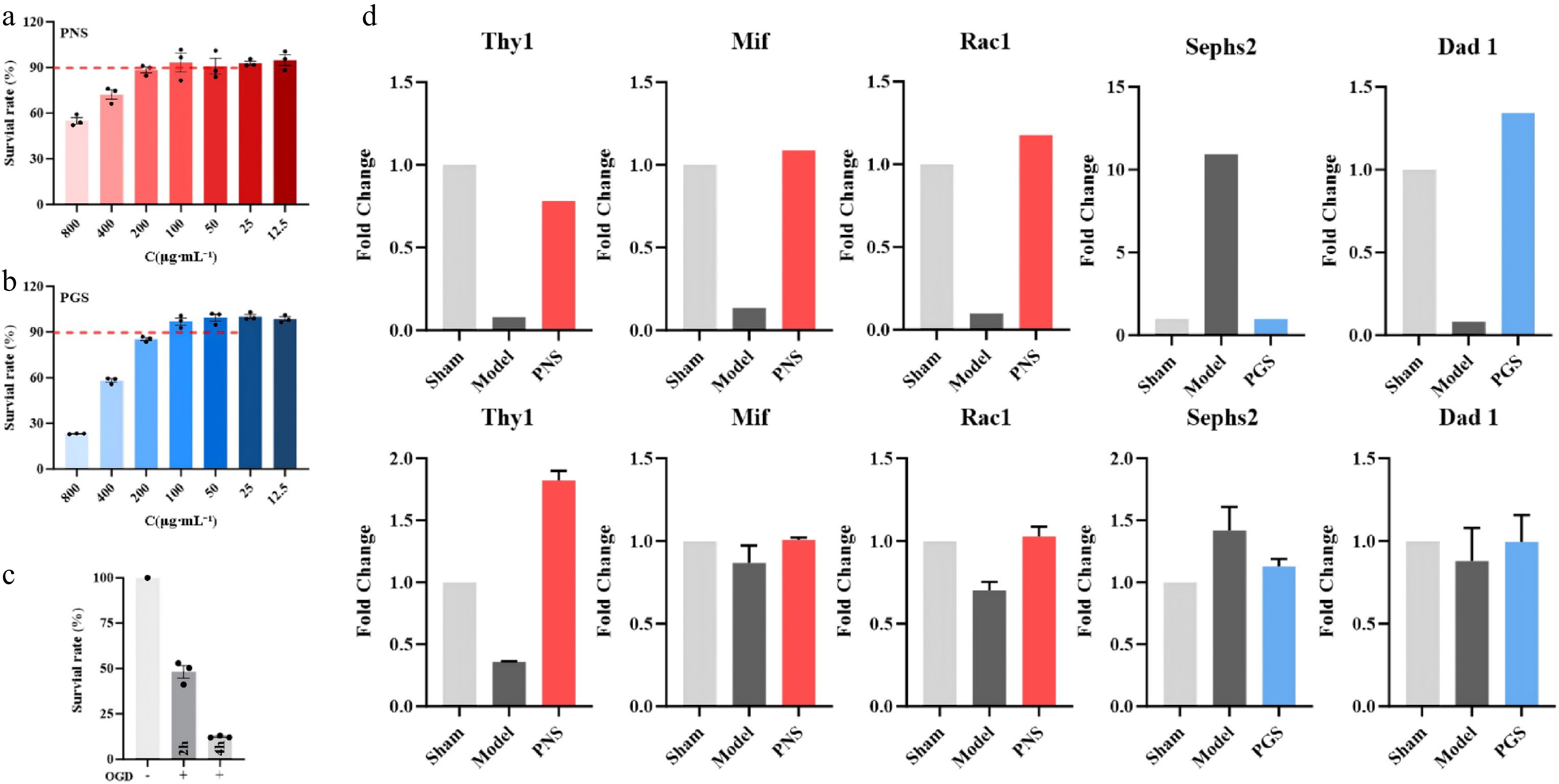
Figure 3. 

qRT-PCR validation of Spatial-seq-derived candidate genes. (a) Dose screening of PNS in BV2 cells. The red dashed line indicates the predefined safety threshold for cell viability (> 90%). (b) Dose screening of PGS in BV2 cells. The red dashed line indicates the predefined safety threshold for cell viability (> 90%). (c) Optimization of OGD duration in BV2 cells. (d) qRT-PCR validation of representative differentially expressed genes identified by Spatial-seq. Candidate genes were selected based on differential expression analysis (|log₂FC| > 1, adjusted P < 0.05) and biological relevance to cerebral ischemia. Validation was performed in BV2 cells, primary neurons, bEnd.3 cells, and mouse ischemic penumbra tissues. Data are presented as mean ± SD, n = 3. Statistical analyses were performed using one-way ANOVA followed by Tukey's multiple-comparison test. Statistical significance was defined as P < 0.05.

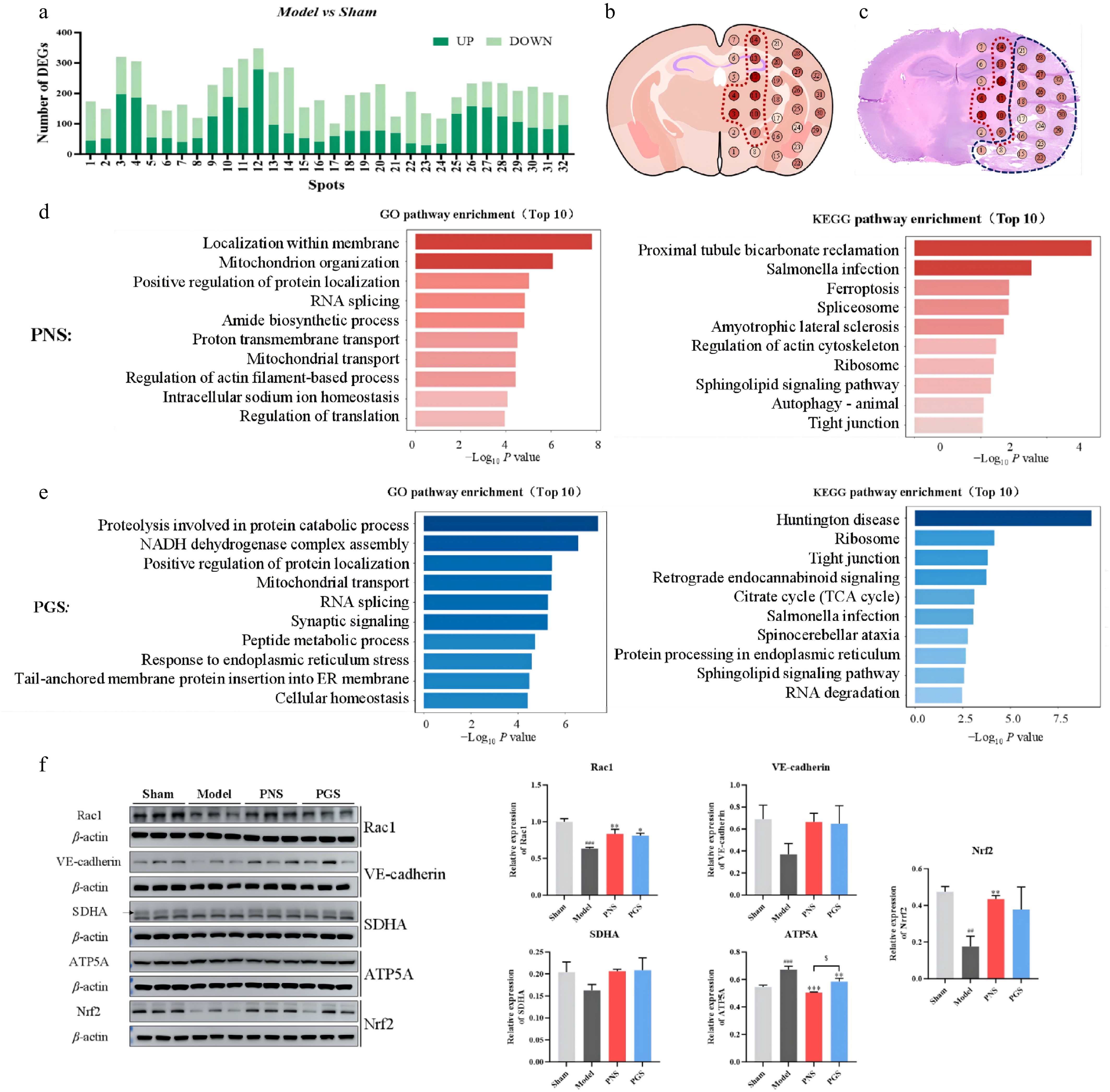
Figure 4. 

Spatial identification of ischemic penumbra-associated regions, functional enrichment analysis, and protein-level validation of representative targets. (a) Stacked histogram of the number of DEGs in 32 spatial spots when comparing the Model group with the Sham group. Dark green indicates upregulated genes and light green indicates downregulated genes. (b) Spatial localization of the 32 numbered spatial spots projected onto a coronal mouse brain reference map. Each circle represents an individual Spatial-seq spot and is labeled according to its spot identification number. The light-to-dark red color gradient represents increasing numbers of DEGs per spatial spot, with darker colors indicating higher DEG abundance. The red dotted contour outlines the top 25% of spots (eight of 32) ranked by DEG number, which were selected as key stroke-associated spatial regions for subsequent analyses. (c) Spatial registration of the 32 numbered spatial spots with the corresponding H&E-stained brain section. Spot colors follow the same DEG-count scale shown in (b). The red dotted contour indicates the ischemic penumbra, whereas the blue dotted contour indicates the infarct core. The spatial registration illustrates the anatomical correspondence between the selected high-DEG spatial spots and histopathological regions of ischemic injury. (d) GO biological process (left) and KEGG pathway (right) enrichment analyses of representative DEGs regulated by PNS within the ischemic penumbra. (e) GO biological process (left) and KEGG pathway (right) enrichment analyses of representative DEGs regulated by PGS within the ischemic penumbra. (f) Representative Western blot images (left) and densitometric quantification (right) of Rac1, VE-cadherin, SDHA, ATP5A, and Nrf2 protein expression in ipsilateral ischemic penumbra tissue collected 24 h after pMCAO. Actin served as the loading control, and protein expression levels were normalized to Actin. Each lane represents one biologically independent sample. Bars represent the Sham (light gray), Model (dark gray), PNS (red), and PGS (blue) groups. Data are presented as mean ± SEM, n = 3. Statistical analyses were performed using one-way ANOVA followed by Dunnett's multiple-comparisons test. ^# P < 0.05; ^## P < 0.01; ^### P < 0.001 vs the Sham group; * P < 0.05, ** P < 0.01; *** P < 0.001 vs the model group; ${}^{\$} $ P < 0.05 indicates comparisons between the PNS and PGS groups.

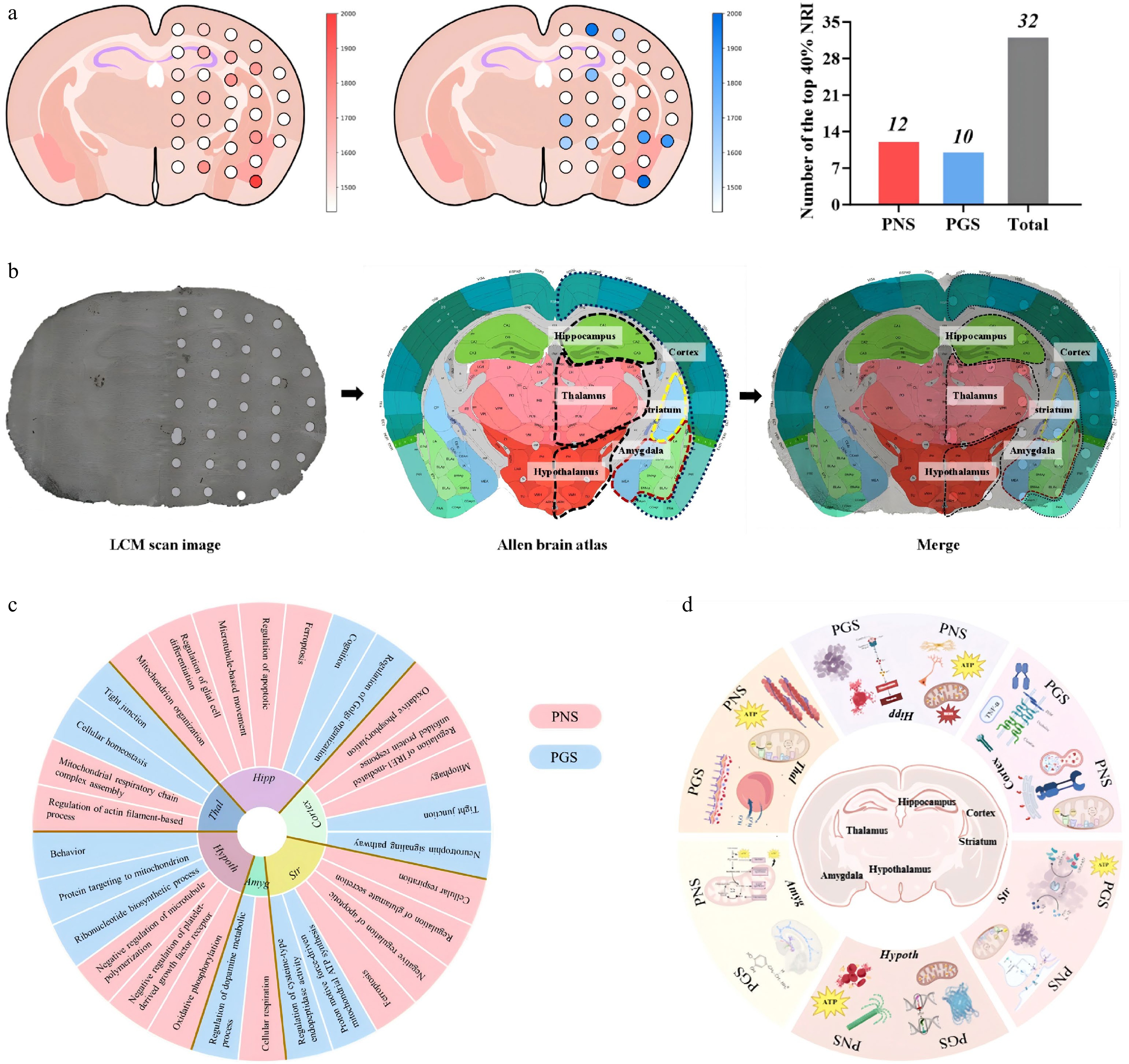
Figure 5. 

Identification of key spatial regions regulated by PNS and PGS and their region-specific functional characterization. (a) Identification of key spatial regions regulated by PNS and PGS using the NRIODN algorithm. Spatial spots are projected onto a coronal mouse brain map. The red color gradient indicates increasing NRIODN scores for PNS-regulated spots, whereas the blue color gradient indicates increasing NRIODN scores for PGS-regulated spots. Darker colors represent greater regional intervention potential. The bar graph summarizes the numbers of key spatial regions identified for each treatment. (b) Registration of Spatial-seq spots to the Allen Mouse Brain Atlas. Left, representative tissue section with the corresponding spatial spot distribution. Middle, anatomical annotation generated from the Allen Brain Atlas reference. Right, overlay of the histological section with the annotated brain atlas after spatial registration. Colored contours delineate major anatomical regions, including the hippocampus, cortex, striatum, thalamus, hypothalamus, and amygdala, which were used for region-specific downstream analyses. (c) GO biological process enrichment analysis of representative marker genes identified in different brain regions. Functional enrichment analysis was performed using Metascape based on a hypergeometric test with Benjamini–Hochberg multiple-testing correction. Only enriched terms with adjusted P < 0.05 were retained. The circular heatmap summarizes representative biological processes enriched in each anatomical region. Pink sectors indicate PNS-associated enrichment, whereas light blue sectors indicate PGS-associated enrichment. (d) Schematic summary of the region-specific biological processes regulated by PNS and PGS across different brain regions. The central diagram illustrates the anatomical distribution of the analyzed regions, whereas the surrounding panels summarize representative biological functions and signaling pathways identified by enrichment analysis.

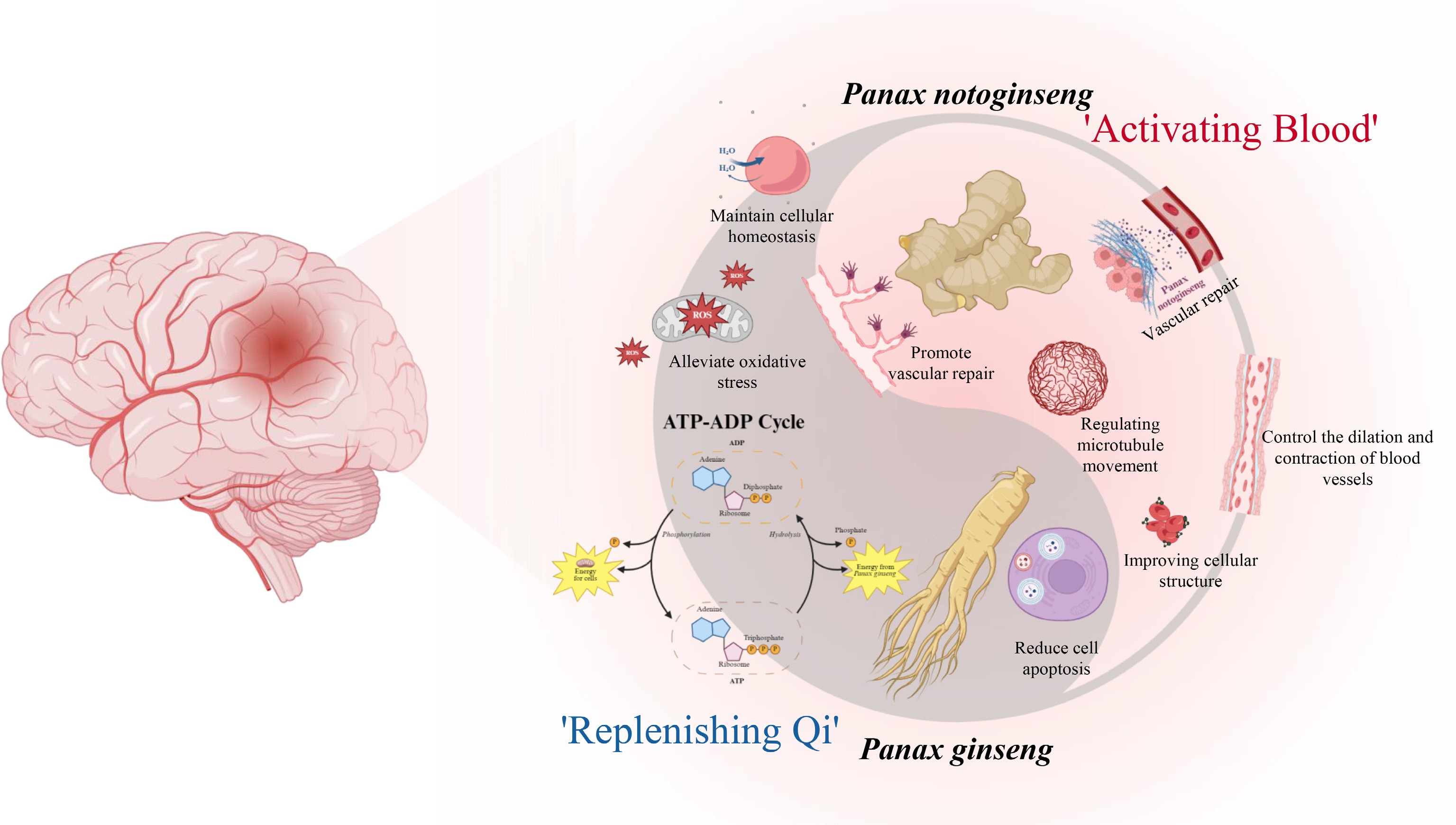
Figure 6. 

Schematic summary of the distinct yet complementary neuroprotective mechanisms of PNS and PGS in acute ischemic stroke. PNS preferentially promotes vascular repair, cytoskeletal remodeling, and vascular homeostasis, consistent with the TCM concept of 'activating blood'. In contrast, PGS predominantly enhances mitochondrial energy metabolism, ATP production, and cellular recovery, consistent with the TCM concept of 'replenishing qi'. Both treatments contribute to the attenuation of oxidative stress and apoptosis.