-
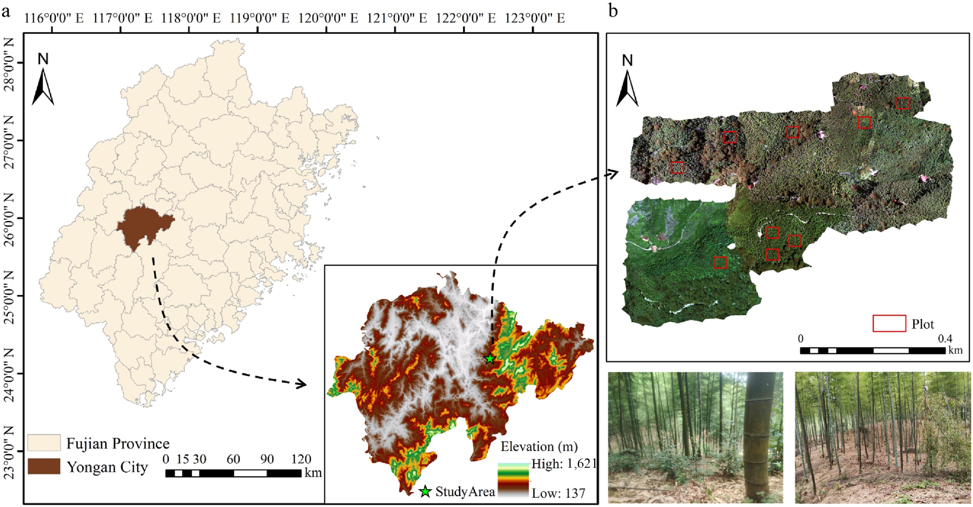
Figure 1.
Spatial location of the study area and field sampling plots. Panel (a) shows the geographic context: The administrative boundary of Fujian Province, the location of Yong'an City, and the elevation map of Yong'an City, with the UAV survey site marked by a green star; the elevation gradient ranges from 137 m (low) to 1,621 m (high). Panel (b) presents the UAV orthoimage covering Shangping Township, Yong'an City, with the nine sample plots delineated by red rectangular frames; the horizontal scale bar represents the distance of the survey area. The two photographs at the bottom illustrate the on-site conditions of the Moso bamboo forest within the sampling plots. The figure is prepared based on a standard map (review number GS [2020]4619), downloaded from the Standard Map Service website of the Ministry of Natural Resources of China. No modifications have been made to administrative boundaries.
-
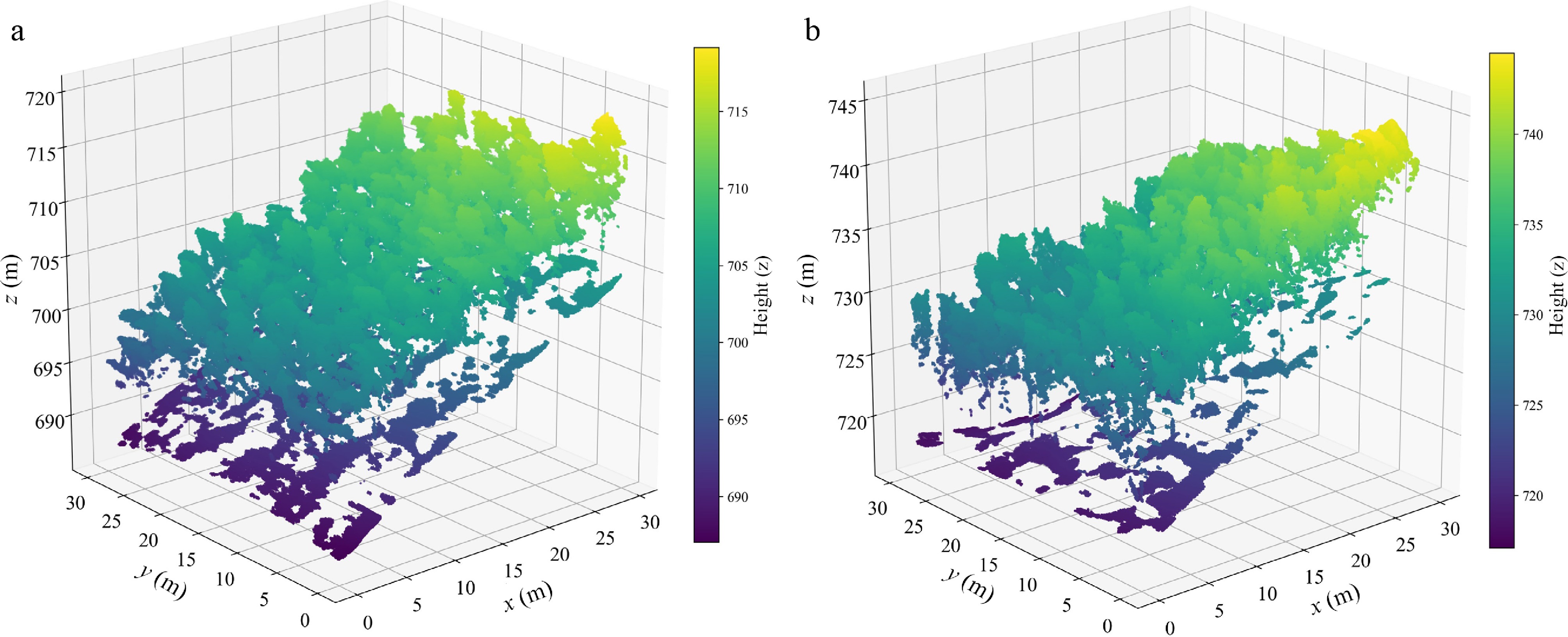
Figure 2.
Three-dimensional visualization of UAV–LiDAR point clouds from two representative Moso bamboo sample plots. (a) Plot YD5; (b) Plot YD6. The horizontal x and y axes represent teh horizontal planar distance (m), and the vertical z axis denotes elevation (m). The color of the point clouds is coded according to the elevation values. The figure demonstrates the complex vertical canopy structure, characterized by high canopy closure and severe inter-culm occlusion in Moso bamboo stands.
-
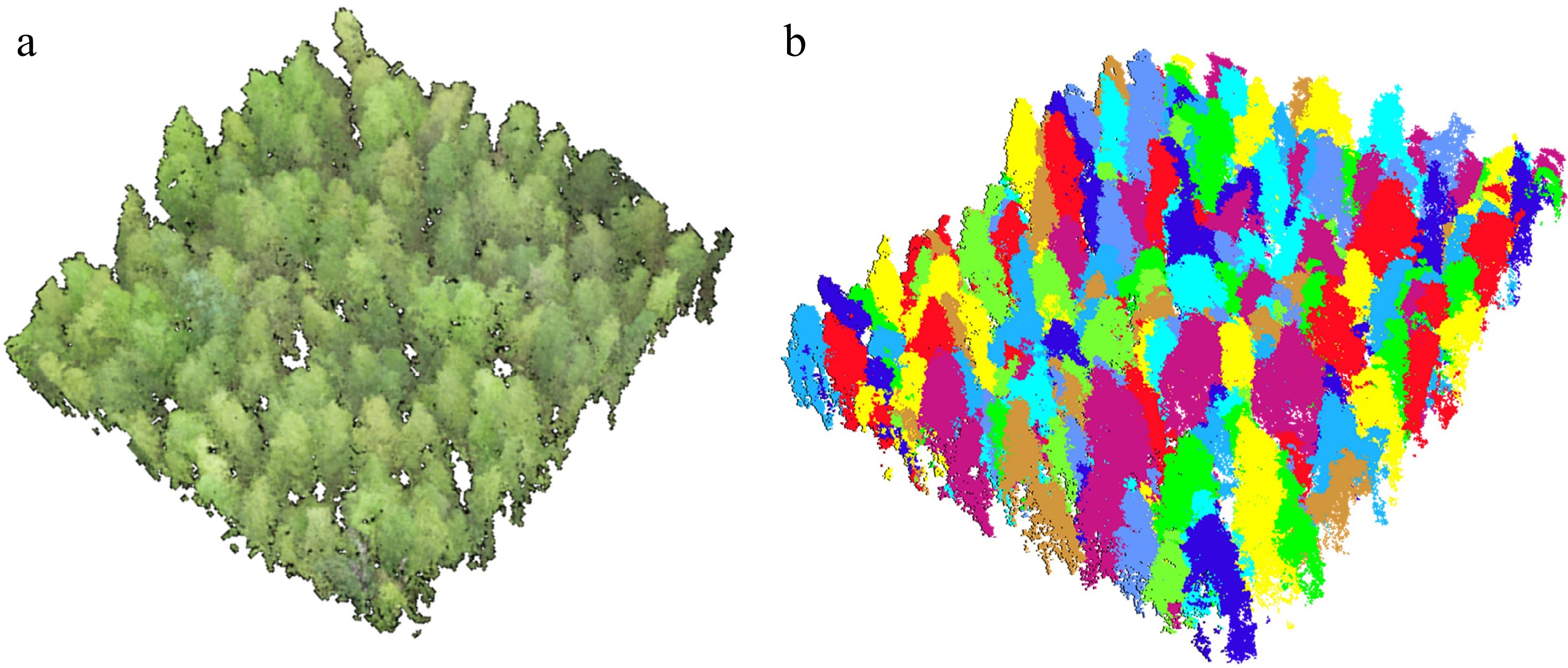
Figure 3.
Point cloud normalization and individual bamboo segmentation using the point cloud segmentation (PCS) algorithm. (a) Normalized point cloud (example: Plot 5); (b) individual bamboo segmentation result based on PCS (example: Plot 5).
-
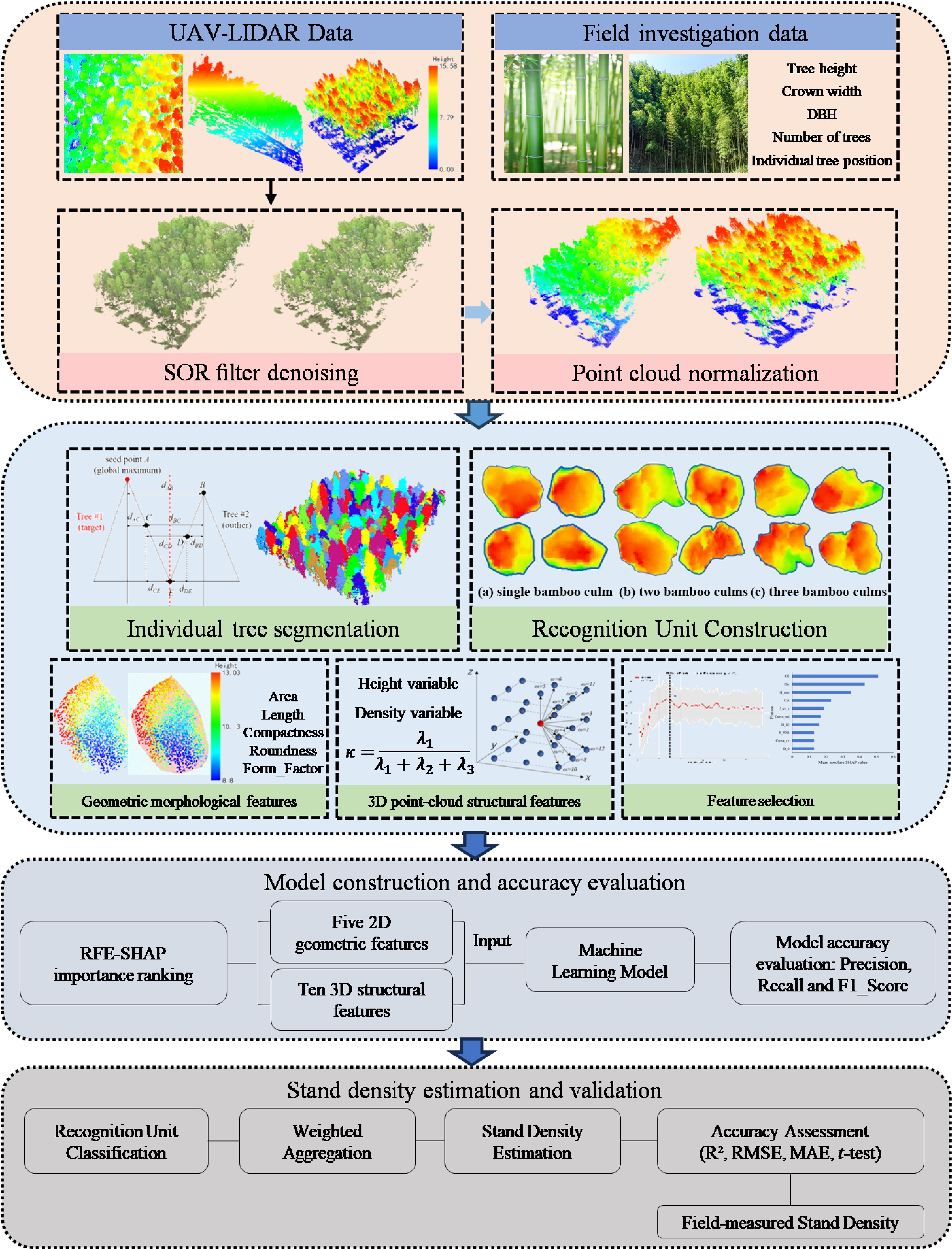
Figure 4.
Technical flowchart.
-
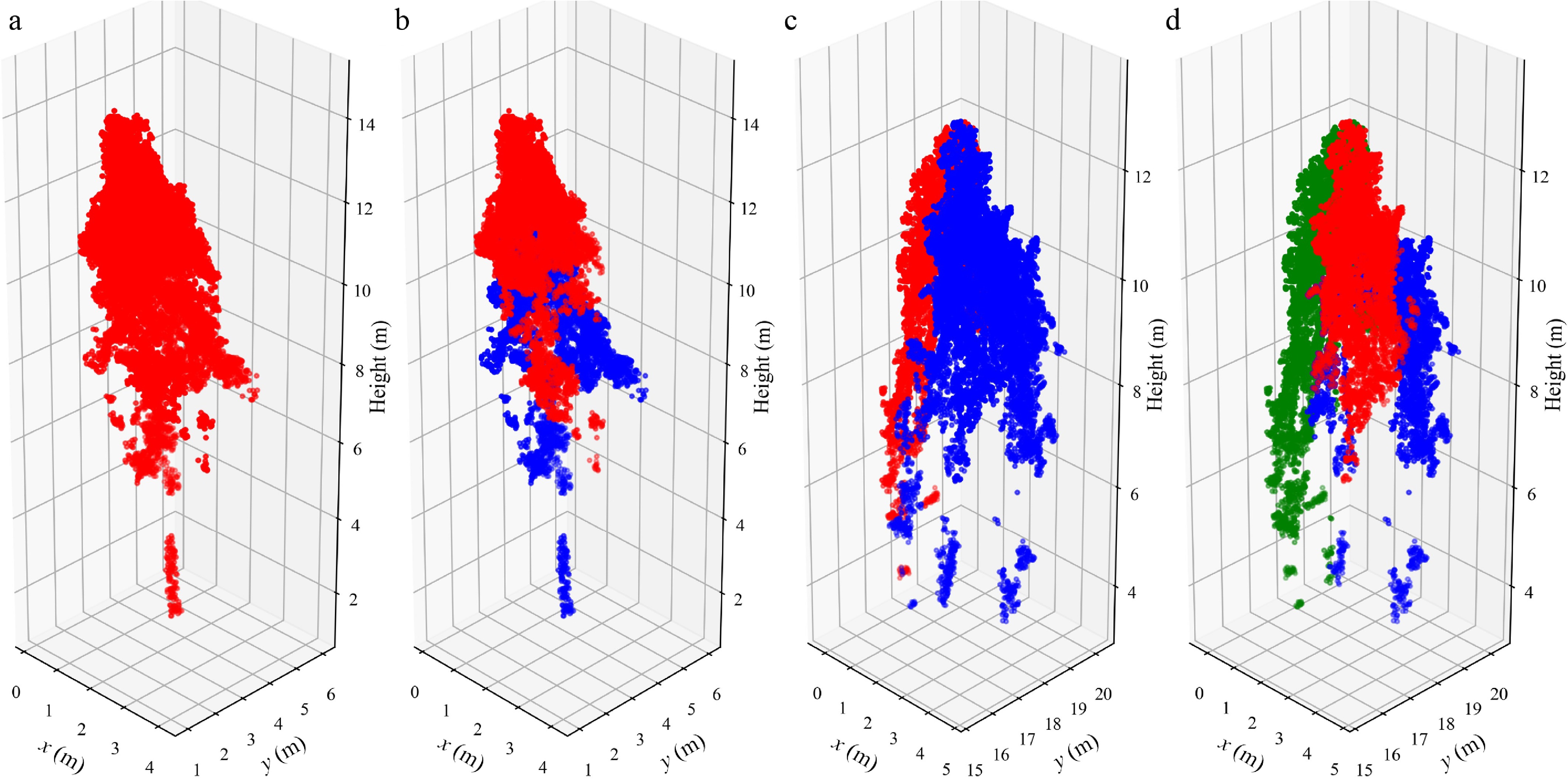
Figure 5.
Examples of inaccurate PCS segmentation results. (a) PCS segmentation result (Example 1); (b) corresponding field-observed culms (Example 1); (c) PCS segmentation result (Example 2); (d) corresponding field-observed culms (Example 2).
-

Figure 6.
Recognition units of different forms of bamboo. (a1), (a2) Single-culm recognition unit; (b1), (b2) two-culm recognition unit; (c1), (c2) three-culm recognition unit.
-
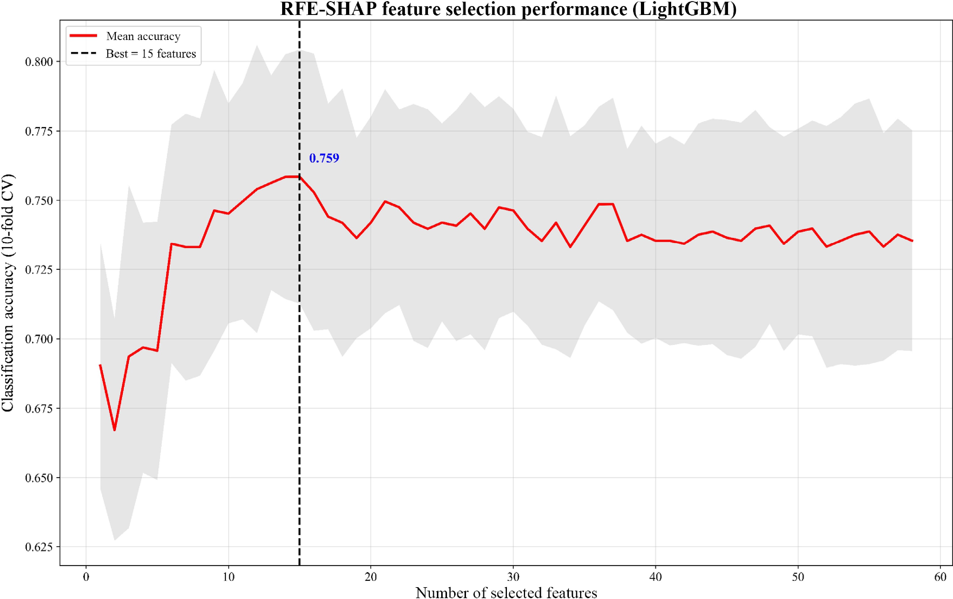
Figure 7.
RFE-SHAP feature selection performance assessment.
-
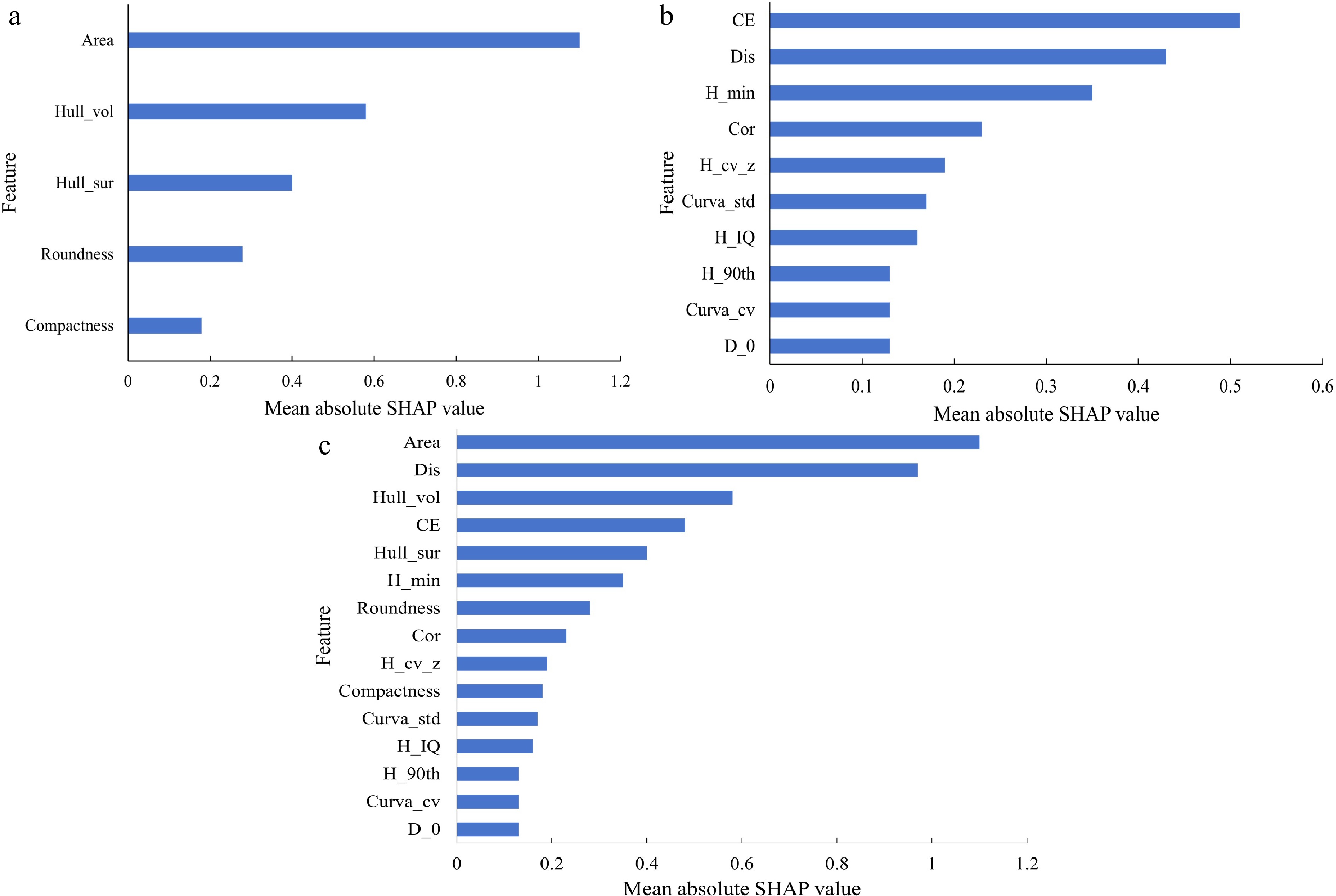
Figure 8.
Results of feature selection using RFE-SHAP. (a) Top 5 geometric descriptors; (b) top 10 point cloud structural features; (c) 15 integrated features.
-
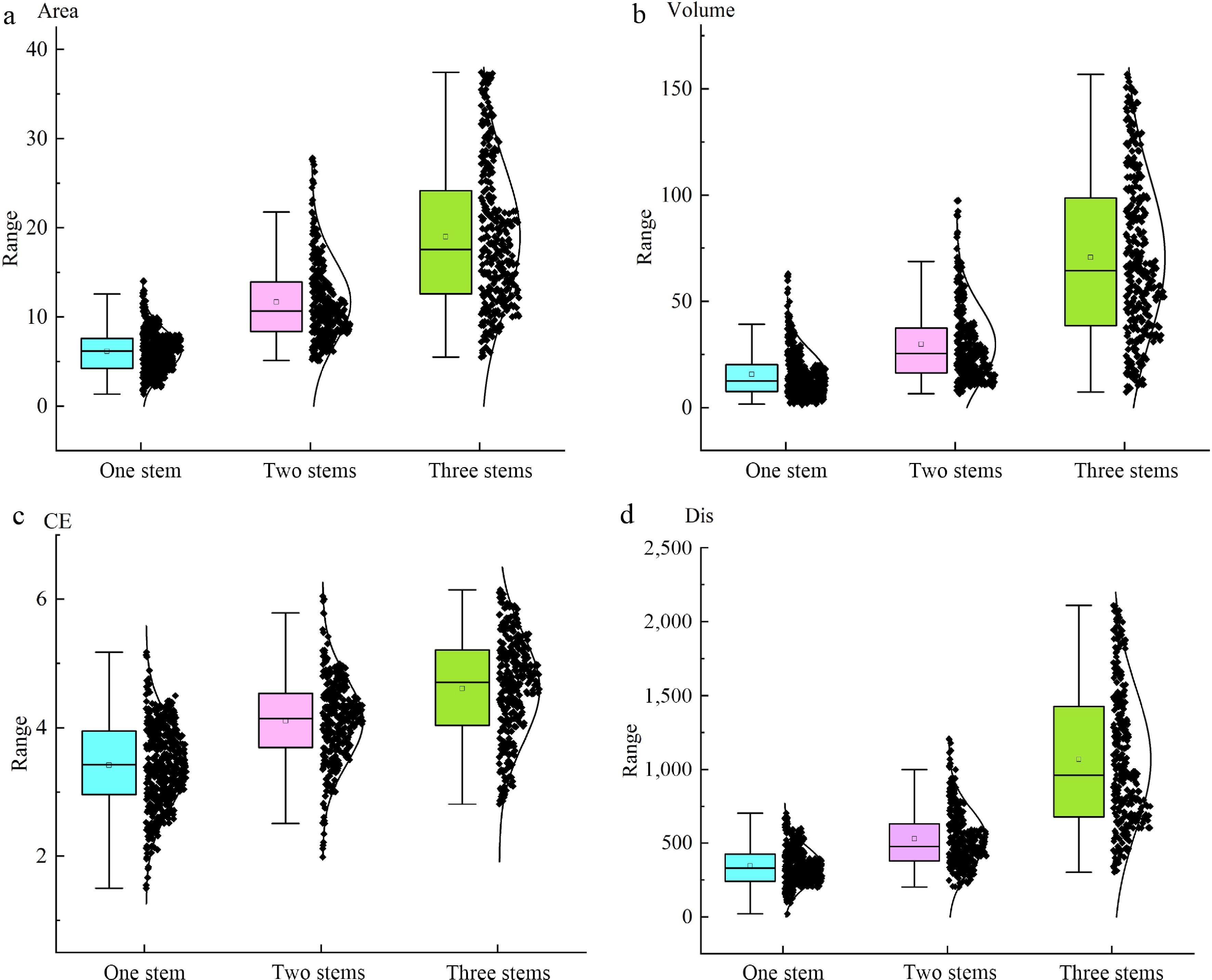
Figure 9.
Feature differences among different recognition units (single, two, and three culms). (a) Area; (b) Hull_Vol; (c) CE; (d) dissimilarity (Dis).
-
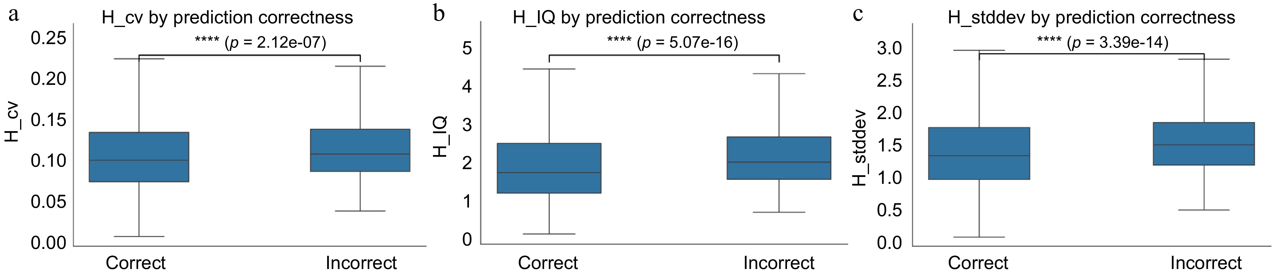
Figure 10.
Comparison of height dispersion metrics between correctly and incorrectly classified recognition units. (a) Coefficient of variation of height (H_cv); (b) interquartile range of height (H_IQ, m); (c) standard deviation of height (H_stddev, m). The Mann–Whitney U-test was adopted to detect statistical differences between groups. Horizontal lines with significance markers denote significant differences between the two groups (****, p < 0.001). H_cv represents the coefficient of variation of point height within each recognition unit; H_IQ is the interquartile range of point height; H_stddev denotes the standard deviation of point height.
-
Sample plot No. Mean culm height (m) Mean DBH (cm) Mean internode length at breast height (cm) Stand density (culms ha−1) Slope (°) Aspect Altitude (m) 1 12.0 10.5 18.9 3,124 39 Northwest 757 2 15.3 10.9 21.1 1,768 28 West 784 3 11.0 9.6 18.9 3,368 20 Southeast 709 4 11.3 9.6 19.4 2,646 30 South 689 5 12.0 8.4 17.4 1,734 35 Northwest 695 6 12.1 8.6 17.9 2,190 22 Northwest 721 7 13.4 10.3 19.2 3,413 32 Northwest 685 8 12.6 10.3 19.5 1,756 19 Northwest 713 9 13.9 10.1 19.7 2,590 29 South 771 Table 1.
Structural and topographic characteristics of the nine sample plots.
-
Morphological features Description Area Total area of the polygon, minus the area of the holes Length The combined length of all boundaries of the polygon, including the boundaries of the holes Compactness A shape measure that indicates the compactness of the polygon. A circle is the most compact shape with a value of 1/π. The compactness value of a square is 1/2(√π).
Compactness = √(4 × area/π) / outer contour lengthRoundness A shape measure that compares the area of the polygon to the square of the maximum diameter of the polygon. The "maximum diameter" is the length of the major axis of an oriented bounding box enclosing the polygon. The roundness value for a circle is 1, and the value for a square is 4/π
Roundness = 4 × (area)/(π × major_length2)Form factor A shape measure that compares the area of the polygon to the square of the total perimeter. The form factor value of a circle is 1, and the value of a square is π/4
Form factor = 4 × π × (area)/(total perimeter2)Hull_Sur Total area of the triangulated mesh of the concave hull reconstructed from the point cloud Hull_Vol Volume enclosed by the concave hull mesh Table 2.
Morphological description of different geometric features.
-
Category Variable Descriptions Height variable Hx Height percentiles H_IQ, H_Sq Interquartile range of height, quadratic mean of height Hmax, Hmean, Hmin, Hmedian Maximum, mean, minimum, and median height Hcv, Hkurtosis, Hskewness, Hstddev, Hvariance Coefficient of variation, kurtosis, skewness, standard deviation, and variance of height Density variable D0, D1, …, D9 Proportion of points in each vertical layer relative to the total number of points, counted from bottom to top X takes values of 1, 5, 10, 20, 25, 30, 40, 50, 60, 70, 75, 80, 90, 95, 99, D0−D9 is the density of the point cloud in each of the ten horizontal layers uniformly divided from low to high. Subscripts such as max, mean, and std indicate the corresponding statistical operations. Table 3.
List of variables extracted from UAV–LiDAR point clouds.
-
Feature category Variable Descriptions Canopy feature CE Canopy entropy 3D texture features Asm Angular second moment Cont Contrast Entr Entropy Idm Inverse difference moment Mean Mean Hom Homogeneity Dis Dissimilarity AutoCor Autocorrelation Cor Correlation Curvature features Curva_Mean Mean curvature Curva_Median Median curvature Curva_PCT90 90th percentile curvature Curva_std Standard deviation of curvature Curva_cv Coefficient of variation of curvature Table 4.
Point clouds' structural features.
-
Feature set Model Accuracy F1
(Single culm)F1
(Two culms)F1
(Three culms)Geometric RF 0.76 0.87 0.69 0.60 SVM 0.67 0.78 0.58 0.56 KNN 0.71 0.82 0.61 0.62 Structural RF 0.74 0.80 0.71 0.65 SVM 0.67 0.73 0.62 0.64 KNN 0.70 0.74 0.66 0.67 Combined RF 0.80 0.92 0.69 0.75 SVM 0.75 0.84 0.66 0.69 KNN 0.79 0.85 0.71 0.71 Table 5.
Classification performance of different feature sets and machine learning models.
-
Recognition unit Single
culmTwo
culmsThree
culmsTotal Producer's
accuracy (%)Single culm 121 9 0 130 93.08 Two culms 12 73 11 96 76.04 Three culms 0 32 64 96 66.67 Total 133 114 75 322 − User's accuracy (%) 90.98 64.04 85.33 Total accuracy (%) − − − − 80.12 Kappa coefficient − − − − 0.698 Overall accuracy = 80.12%; Kappa = 0.698. Rows correspond to the true reference classes, and columns correspond to the model-predicted classes. Row totals indicate the number of samples for each true class, and column totals indicate the number of samples assigned to each predicted category. Diagonal values represent correctly classified samples; off-diagonal values denote misclassified samples. Table 6.
The RF model's identification results.
-
Variable Mean
(culms plot−1)Standard deviation (culms plot−1) Standard error (culms plot−1) t df p Measured vs. predicted −9.78 16.10 5.37 −1.82 8 0.11 Table 7.
Results of the paired-sample t-test between predicted and field-measured culm counts at the plot level.
-
Sample
plot No.Measured culms
(culms plot−1)Predicted culms
(culms plot−1)Relative error (%) PCS culms (culms plot−1) Relative error (%) 1 281 295 5.0 189 32.7 2 159 183 15.1 164 3.1 3 303 290 4.3 256 15.5 4 238 257 8.0 207 13.0 5 156 167 7.1 181 16.0 6 197 216 9.6 159 19.3 7 307 285 7.2 229 25.4 8 158 173 9.5 137 13.3 9 233 254 9.0 186 20.2 Mean relative error (%) 8.3 17.6 MAE (culms plot−1) 17.6 42.7 RMSE (culms plot−1) 18.1 50.0 Relative error (%) = |estimated – measured|/measured × 100%, where "measured" is the field-measured culm count per plot (30 m × 30 m), "estimated" is the culm count estimated by recognition units and "PCS estimated culms" are outputs derived by PCS. Table 8.
Comparison of measured and estimated bamboo culm counts using PCS segmentation and the proposed recognition unit method.
-
Variable Spearman p-value Stand density −0.172 0.382 Slope 0.330 0.086 Altitude −0.079 0.690 Table 9.
Plot-level Spearman correlation between mean absolute relative error and site factors.
Figures
(10)
Tables
(9)