-
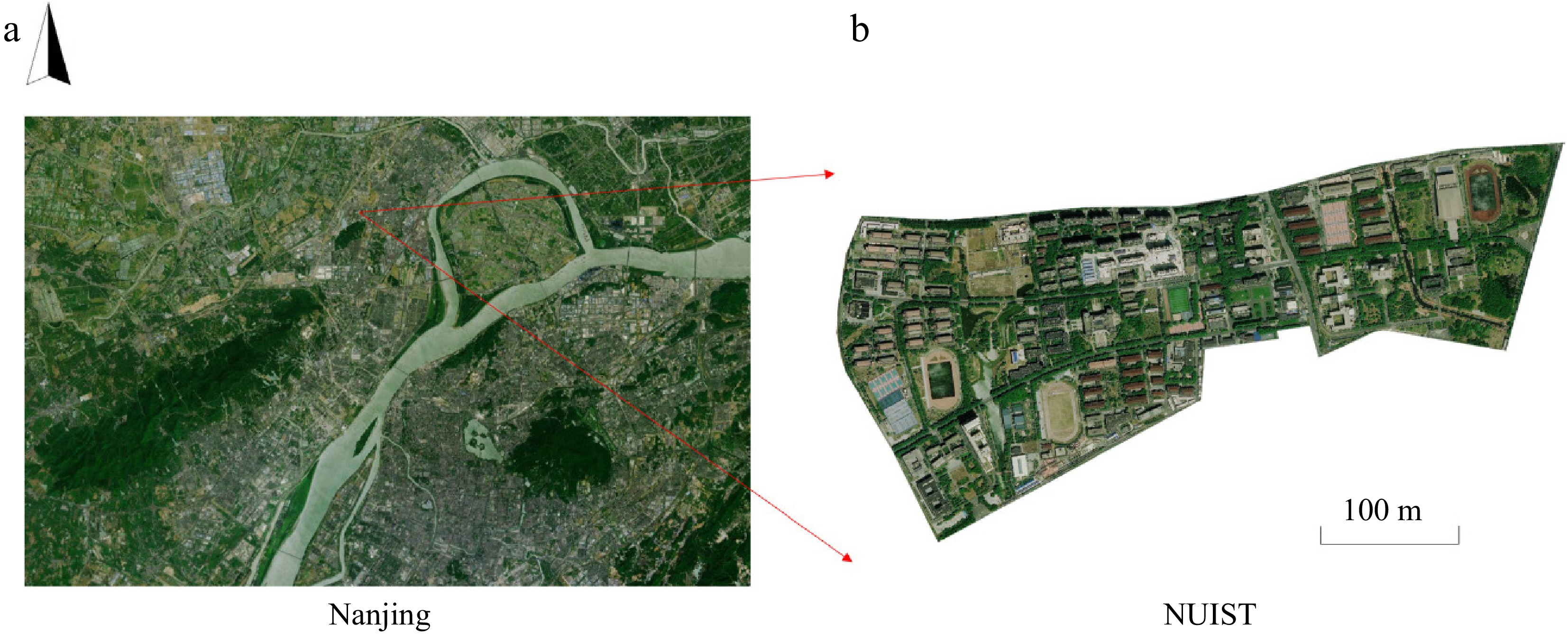
Figure 1.
Area of the NUIST dataset used in this study, located in Nanjing.
-
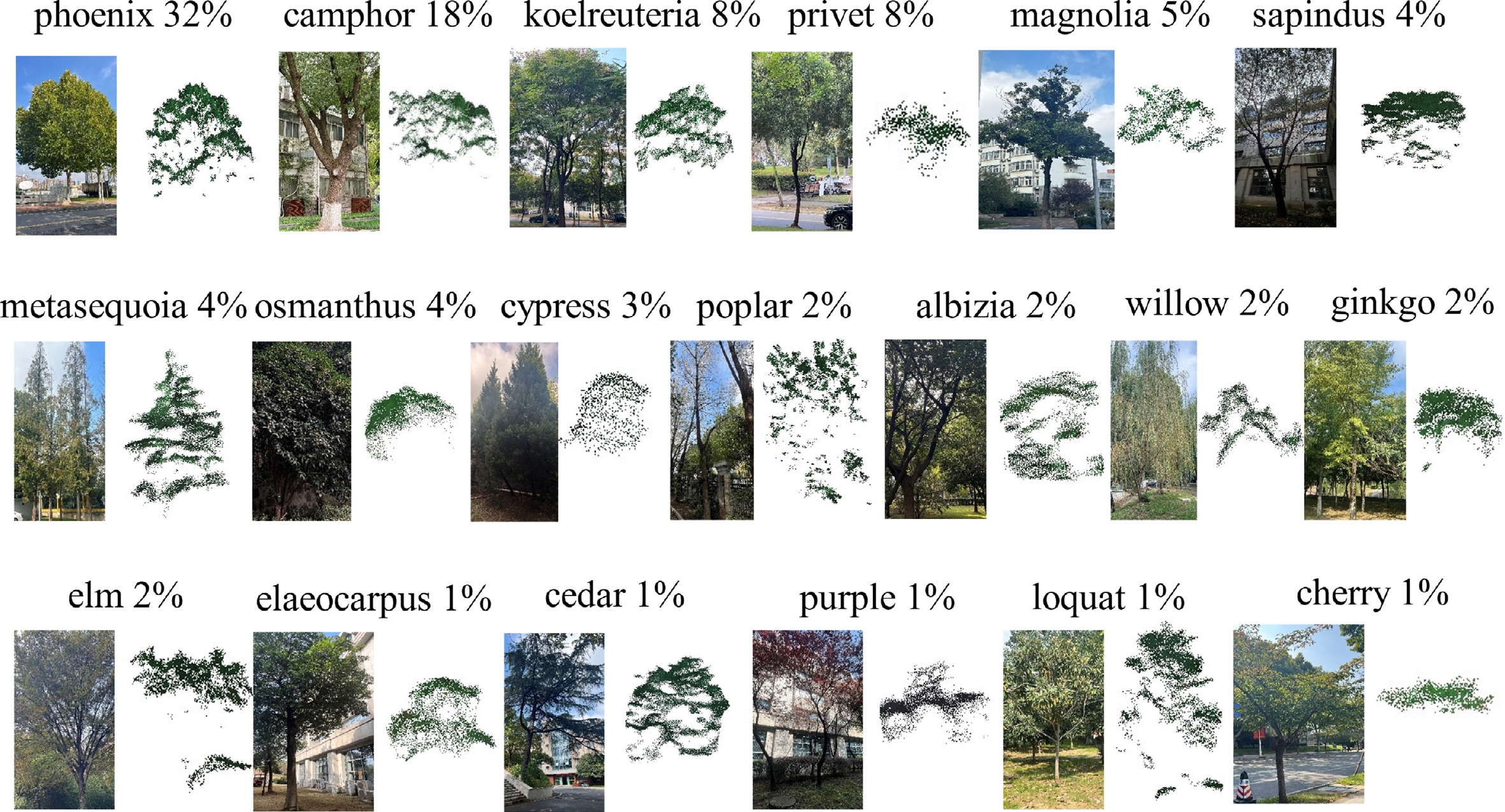
Figure 2.
Representative examples and proportion of training samples of each tree species class.
-
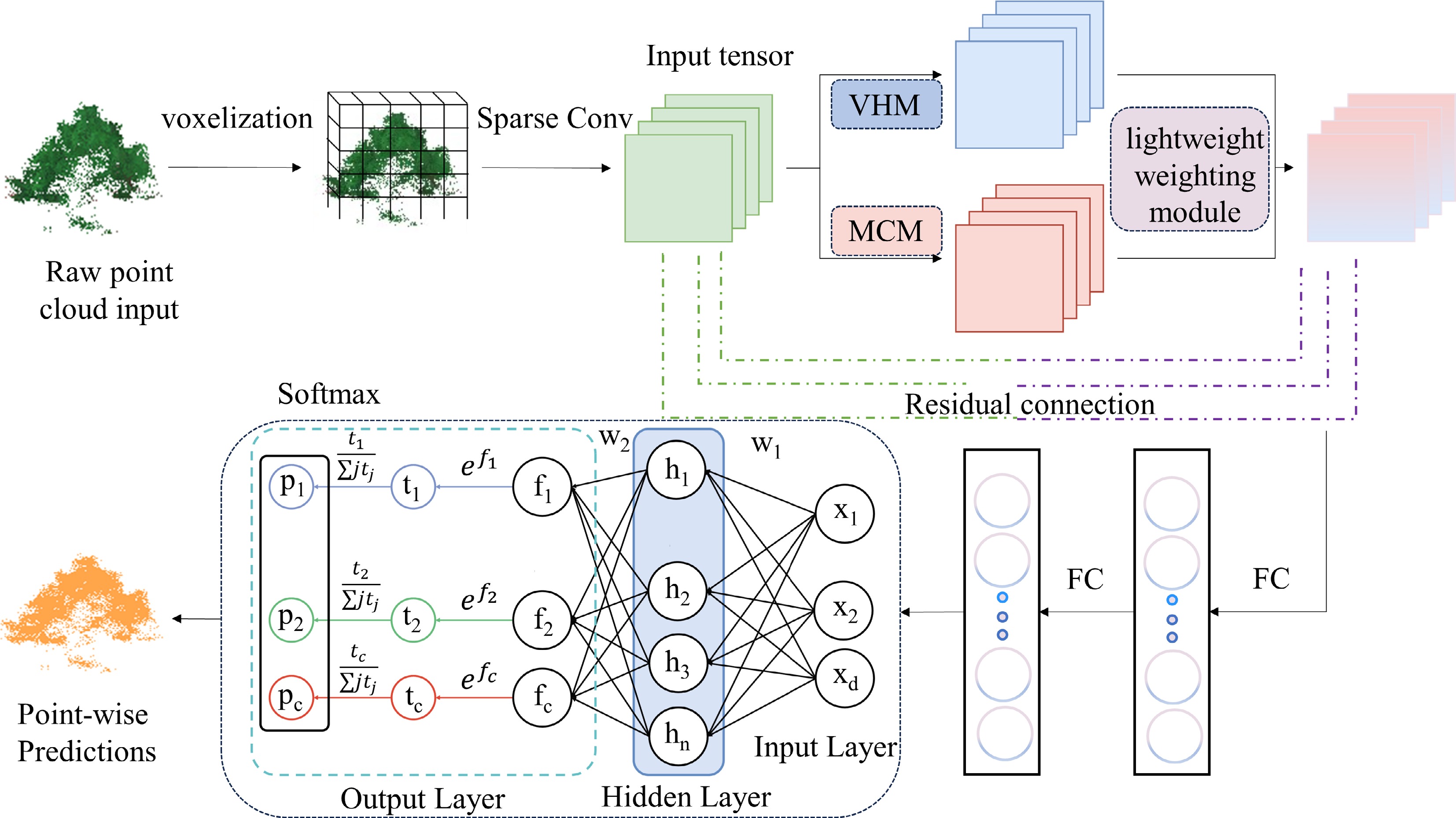
Figure 3.
The TSC-Net framework for classifying tree species.
-
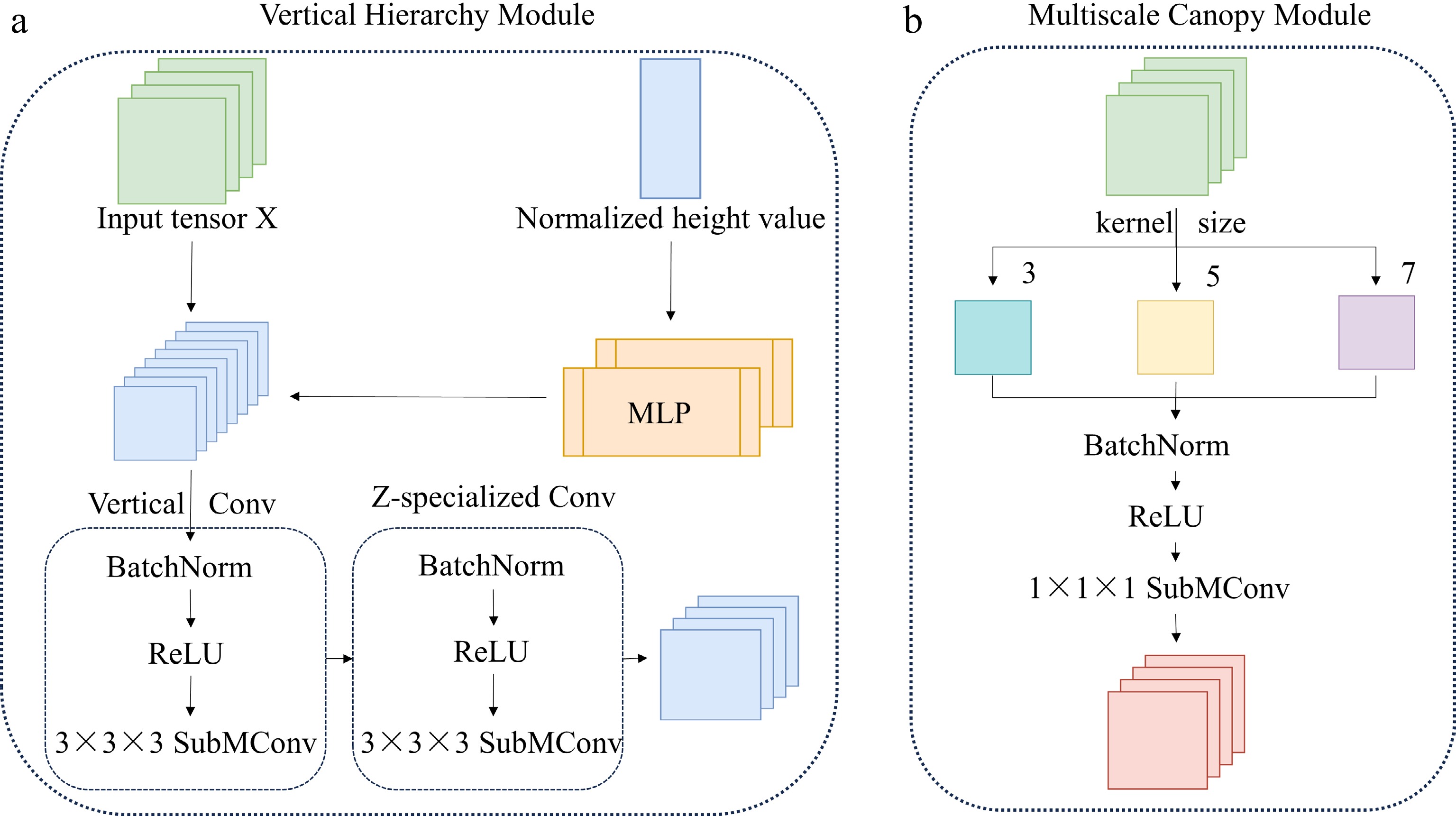
Figure 4.
Workflow of the two modules: (a) VHM; (b) MCM.
-
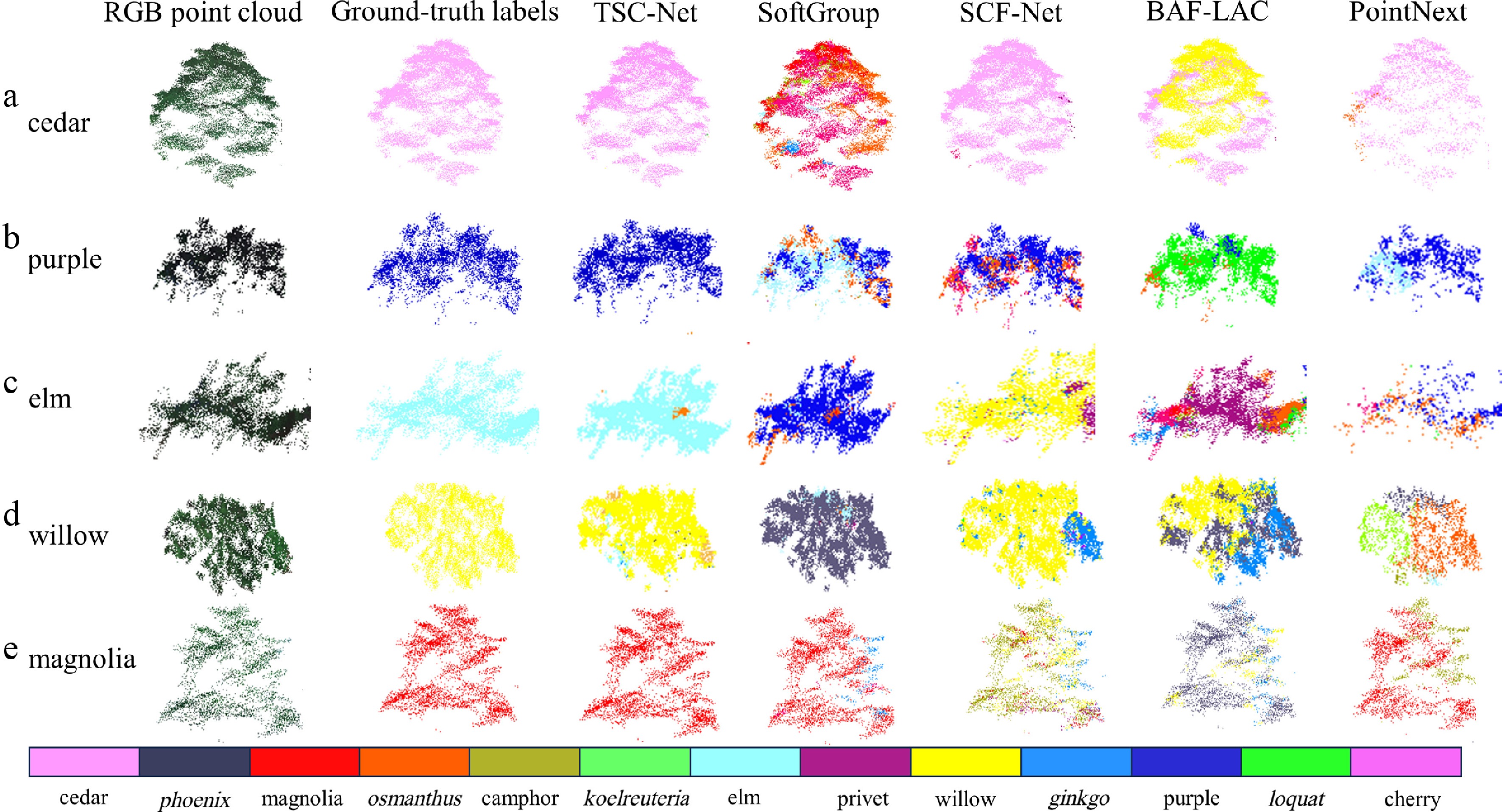
Figure 5.
Visualization of pointwise prediction results on representative canopy cluster samples from the NUIST dataset. The first column shows RGB-colored point cloud renderings used solely for visual reference and does not correspond to the labels' color bar. The second column presents the ground truth species labels, and the other columns show the corresponding predictions generated by the models. The color bar applies only to the ground truth labels and prediction panels.
-
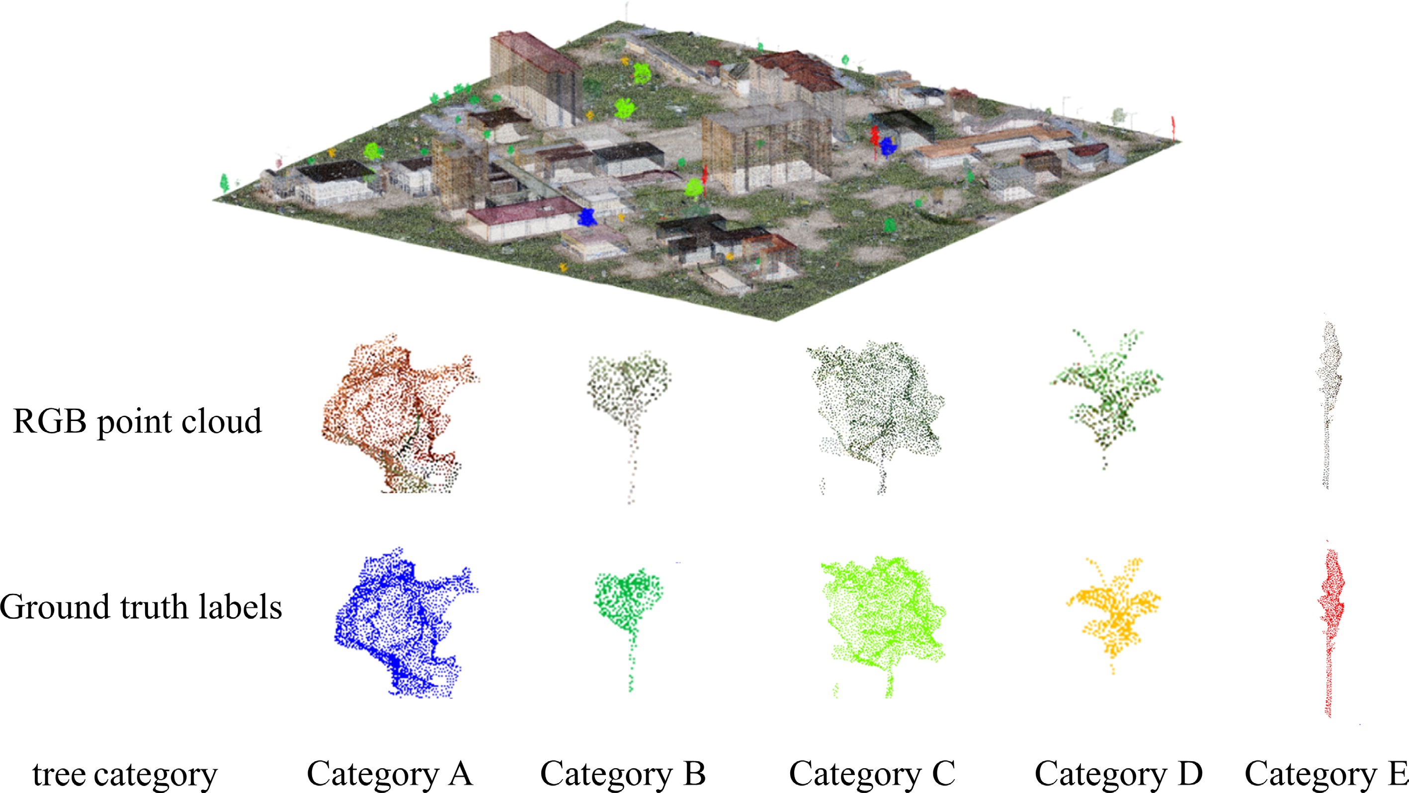
Figure 6.
Visualization of representative tree category samples extracted from the STPLS3D dataset. Since the original STPLS3D dataset provides anonymized tree category labels rather than botanical species names, the samples are denoted as Category A–E instead of specific species names.
-
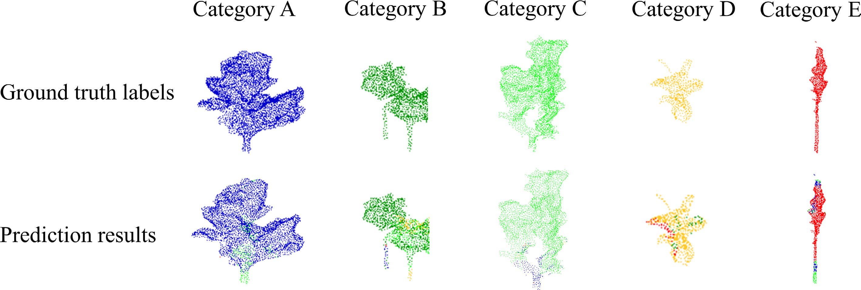
Figure 7.
Qualitative comparison between manually annotated category labels and TSC-Net's predictions on the STPLS3D dataset. The first row shows the ground truth labels, and the second row presents the corresponding predictions generated by TSC-Net.
-
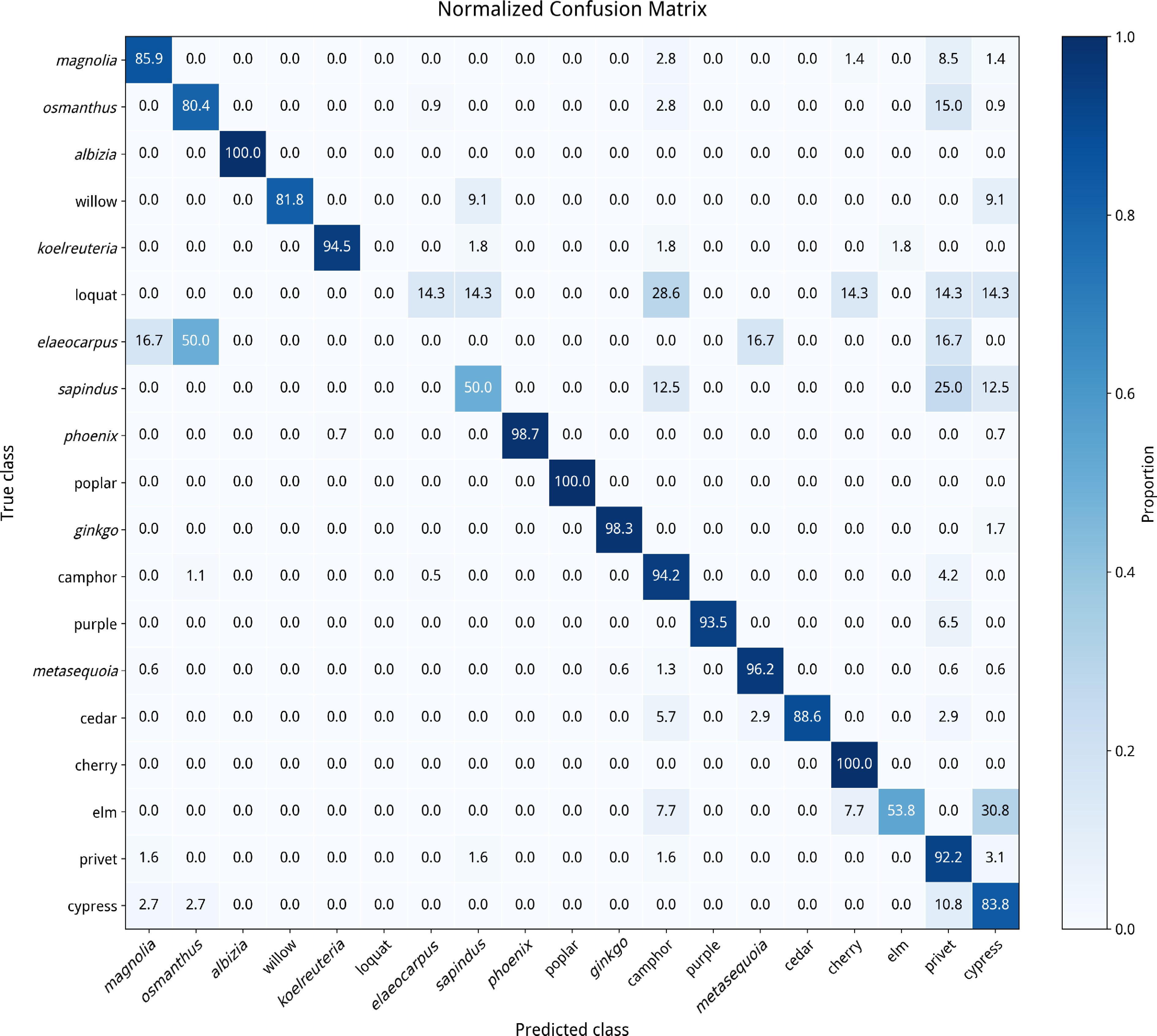
Figure 8.
Row-normalized confusion matrix for canopy-level tree species classification using majority voting. Each row represents the true species, and each column represents the predicted species. Diagonal values indicate the classwise recall, whereas off-diagonal values indicate interspecific misclassification rates.
-
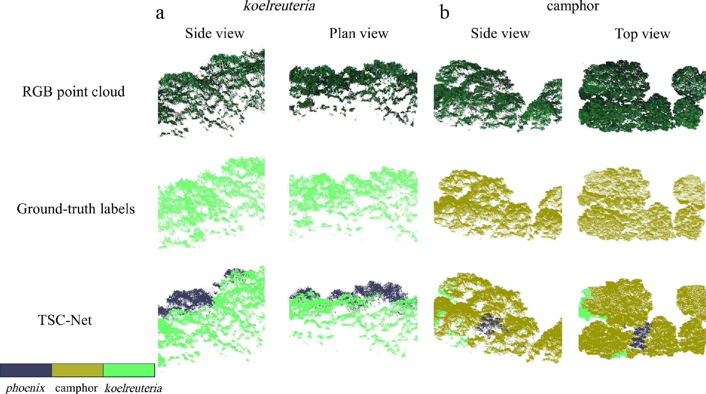
Figure 9.
Visualization of classification results for Phoenix-related errors. (a) Phoenix–Koelreuteria misclassification; (b) Phoenix–camphor misclassification. The first row shows RGB-colored point cloud renderings solely for visual reference and does not correspond to the color bar. The second row presents the ground truth species labels; the third row shows the corresponding predictions generated by TSC-Net. The color bar applies only to the ground truth and prediction panels, where colors represent the three species involved in the confusion analysis: Phoenix, camphor, and Koelreuteria.
-
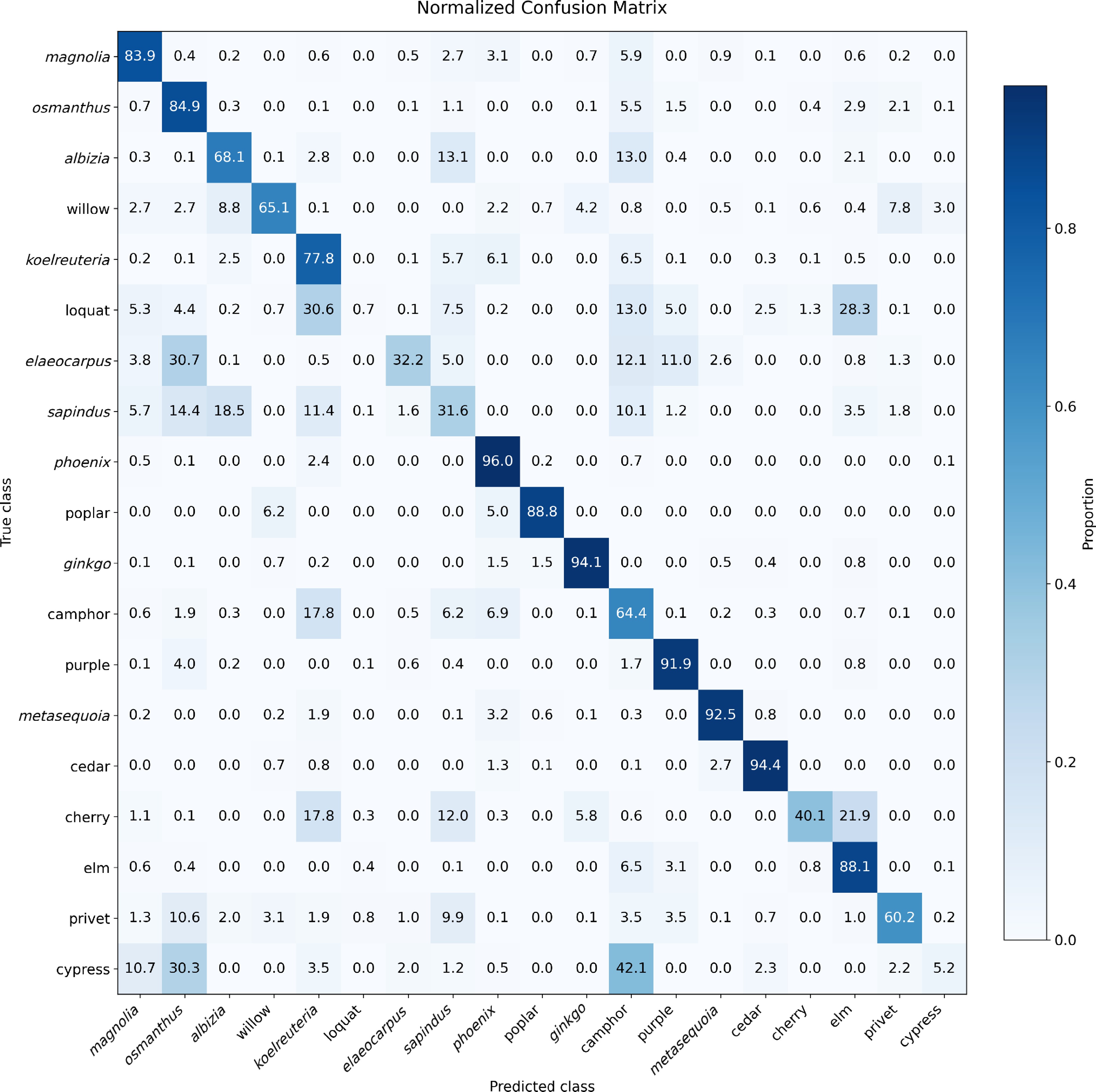
Figure 10.
Row-normalized confusion matrix of TSC-Net on the NUIST test set. The matrix reveals the dominant confusion patterns among minority and visually similar tree species.
-
Tree species class IoU (%) TSC-Net RandLA PointNext SCF-Net BAF-LAC BAAF-Net SPVCNN SoftGroup Random forest mIoU 53.80 26.75 29.63 15.67 21.90 31.35 40.40 38.60 6.50 Magnolia 76.10 26.60 44.71 20.00 65.89 43.92 62.30 66.10 15.10 Osmanthus 67.60 17.13 38.12 3.71 1.77 28.64 71.60 43.60 5.85 Albizia 24.20 28.78 3.90 0.06 15.70 9.56 23.70 0.70 0.56 Willow 45.70 4.46 19.70 5.50 3.39 8.31 14.70 41.40 1.07 Koelreuteria 48.80 29.44 38.21 28.07 27.04 45.59 40.10 64.50 10.61 Loquat 0.60 0.01 4.05 0.00 1.08 0.00 0.00 0.10 0.89 Elaeocarpus 24.40 6.20 8.89 3.41 5.85 0.76 8.80 7.10 1.46 sapindus 11.70 3.01 1.97 0.43 3.72 5.65 40.30 20.70 0.40 Phoenix 87.60 61.61 71.19 70.14 64.40 82.39 47.00 81.50 2.76 Poplar 76.00 68.90 45.27 14.00 14.76 66.53 70.80 6.70 2.10 Ginkgo 90.10 20.70 23.05 1.93 10.13 34.51 67.70 63.60 6.39 Camphor 59.00 39.84 39.53 20.74 27.52 54.11 47.20 64.00 2.98 Purple 78.00 42.45 63.54 56.30 56.00 44.10 76.10 46.90 40.94 metasequoia 89.60 42.32 60.50 25.40 54.00 85.45 92.10 84.90 3.77 Cedar 87.30 49.36 66.75 38.45 48.53 43.98 2.90 67.60 19.63 cherry 34.50 2.40 0.01 0.00 0.00 0.00 35.30 1.20 2.59 elm 62.30 28.76 5.15 0.01 7.00 16.51 42.40 43.00 1.75 privet 53.30 20.71 28.00 9.32 9.00 25.66 24.80 13.00 4.54 Cypress 4.60 1.29 0.53 0.00 0.00 0.00 0.00 16.60 0.12 The number in bold indicates the highest accuracy among all networks. Table 1.
Comparison of pointwise prediction performance on the NUIST campus dataset.
-
Module VHM MCM mIoU (%) iter_time (s) A 38.6% 0.5093 B √ 49.7% 0.6173 C √ 43.2% 0.5363 D √ √ 53.8% 0.5843 Table 2.
Effects of introducing different modules on the NUIST dataset.
-
Tree category Point counts IoU (%) Category A 248,264 86.9 Category B 278,469 71.1 Category C 412,494 86.9 Category D 135,507 53.9 Category E 31,411 16.7 Table 3.
Per-category point counts and IoU in the STPLS3D dataset.
Figures
(10)
Tables
(3)