-
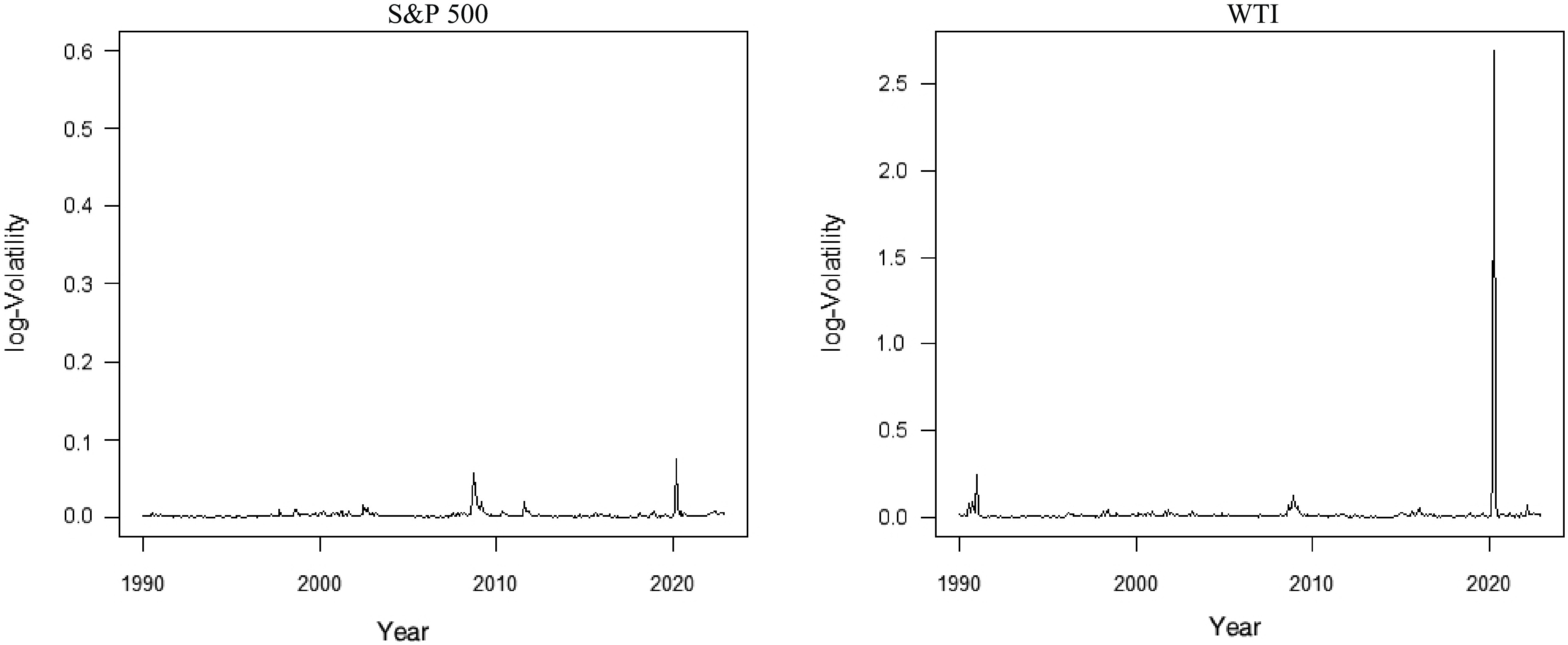
Figure 1.
Realized volatility of oil prices and the S&P 500 index from 1990 to 2022.
-
Grid search for the BAR's threshold parameters Initialization: Set threshold parameters $ {\eta }_{1} $ $ {\eta }_{2} $ $ {\eta }_{1}< {\eta }_{2} $ $ [{\mathrm{a}}_{1},{\mathrm{a}}_{2}] $ Step 1: Define the buffer region width as $ b={\eta }_{2}-{\eta }_{1} $ Step 2: Constrain the buffer size by setting $ b\in (0,\dfrac{{a}_{2}-{a}_{1}}{\mathrm{c}}] $ $ c\in \{5,\;6,\;7,\;8,\;9,\;10\} $ Step 3: Iterate over all possible combinations of $ {\eta }_{1} $ Step 4: Compute the optimal parameters as $ \{ {\eta }_{1},\;b,\;c\}={\mathrm{argmax}}\{R^{2}\;{\text{of the BAR(p) model }}-{R}^{2}\;{\text{of benchmark model}} \} $ Output: The statistically justified optimal threshold values $ {\eta }_{1} $ $ {\eta }_{2} $ Table 1.
Improved grid search algorithm for the BAR model's threshold parameters.
-
Stock Oil Price Return Volatility Price Return Volatility Mean 1,502.645 0.000 0.003 49.825 0.001 0.019 Median 1,252.800 0.001 0.001 45.490 0.001 0.008 Minimum 295.500 −0.128 0.000 10.010 −1.324 0.001 Maximum 4,796.560 0.110 0.075 145.290 0.722 2.691 SD 997.588 0.011 0.006 29.407 0.031 0.136 Skewness 1.301 −0.394 8.360 0.603 −8.435 19.065 Kurtosis 4.252 13.615 91.279 2.272 472.150 373.271 ADF 2.372 −20.459*** −5.649*** 2.561 −18.736*** −6.960*** Notes: ADF, augmented Dickey–Fuller test statistic. The symbols *, **, and *** indicate rejection of the null hypothesis with statistical significance at 10%, 5%, and 1% levels, respectively. Table 2.
Descriptive statistics and tests for a unit root.
-
Coefficient t-statistic Coefficient t-statistic AR(6) Reference ARX(6) Parameter estimation results $ \omega $ −1.214*** −4.996 −1.014*** −3.431 $ {\beta }_{1} $ 0.544*** 10.668 0.349*** 5.206 $ {\beta }_{2} $ 0.125** 2.166 0.310*** 4.521 $ {\beta }_{3} $ 0.002 0.036 0.232** 3.254 $ {\beta }_{4} $ 0.016 0.283 −0.074 −1.047 $ {\beta }_{5} $ 0.049 0.849 −0.015 −0.230 $ {\beta }_{6} $ 0.009 0.183 −0.117 −1.861 $ \beta $ − − 0.078 1.663 Percentage of increase in R2 $ {\Delta \mathrm{R}}^{2} $ − 7.71 TAR(6) $ {V}_{t,stock}\leq -6.999 $ $ {V}_{t,stock}> -6.999 $ Parameter estimation results $ {\beta }_{0} $ −0.763 −1.189 −1.566*** −4.681 $ {\beta }_{1} $ 0.248* 1.905 0.399*** 5.256 $ {\beta }_{2} $ 0.357** 2.286 0.304*** 3.867 $ {\beta }_{3} $ 0.187 1.145 0.215*** 2.652 $ {\beta }_{4} $ 0.104* 2.675 −0.111** −1.873 $ {\beta }_{5} $ 0.081 0.580 −0.047 −0.588 $ {\beta }_{6} $ −0.127 −0.911 −0.099 −1.342 Percentage increase of R2 $ {\Delta \mathrm{R}}^{2} $ − 8.72 Notes: The table reports slope parameter estimates together with the heteroskedasticity- and autocorrelation-consistent t-statistics based on the Newey–West method. The percentage increase in $ {\text{R}}^{2} $ Table 3.
Within-sample estimation results of the AR, ARX, and TAR models for monthly oil volatility.
-
Coefficient t−statistic Coefficient t−statistic AR(6) Reference ARX(6) Parameter estimation results $ \omega $ −1.214*** −4.996 −1.014*** −3.431 $ {\beta }_{1} $ 0.544*** 10.668 0.349*** 5.206 $ {\beta }_{2} $ 0.125** 2.166 0.310*** 4.521 $ {\beta }_{3} $ 0.002 0.036 0.232** 3.254 $ {\beta }_{4} $ 0.016 0.283 −0.074 −1.047 $ {\beta }_{5} $ 0.049 0.849 −0.015 −0.230 $ {\beta }_{6} $ 0.009 0.183 −0.117 −1.861 $ \beta $ − − 0.078 1.663 Percentage of increase in R2 $ {\Delta \mathrm{R}}^{2} $ − 7.71 BAR(6) $ {V}_{t,stock} $ $ {V}_{t,stock} $ Parameter estimation results $ {\gamma }_{0} $ −1.149* −1.786 −1.549*** −4.743 $ {\gamma }_{1} $ 0.154 0.971 0.394*** 5.505 $ {\gamma }_{2} $ 0.317** 2.014 0.296*** 3.838 $ {\gamma }_{3} $ 0.143* 1.932 0.248*** 3.048 $ {\gamma }_{4} $ 0.115 0.778 −0.125 −1.542 $ {\gamma }_{5} $ 0.126 0.719 −0.022 −0.294 $ {\gamma }_{6} $ −0.068 −0.490 −0.129* −1.811 Percentage increase of R2 $ {\Delta \mathrm{R}}^{2} $ − 9.21 Notes: The table reports the slope parameter estimates and Newey–West heteroskedasticity- and autocorrelation-consistent t−statistics. In addition, it shows the percentage of the increase in R2 relative to the baseline AR(6) model in Eq. (2). For the BAR(6) model, two thresholds are reported (−7.104 and −6.999), which define a buffer zone between the regimes and capture the hysteresis effect. The symbols *, **, and *** denote statistical significance at the 10%, 5%, and 1% levels, respectively. Table 4.
Within-sample estimation results of the AR, ARX, and BAR models for monthly oil volatility.
-
Model: ARX(6) Model: TAR(6) Model: BAR(6) Recursive Rolling Recursive Rolling Recursive Rolling 2011−2022 $ \Delta R_{oss}^{2} $ −4.635** −1.168** 6.319*** 5.001*** 8.176*** 6.855*** p−Value 1.63 × 10⁻² 1.4 × 10⁻² 6.76 × 10⁻⁴ 1.66 × 10⁻³ 3.71 × 10⁻⁴ 2.57 × 10⁻⁴ 2013−2022 $ \Delta R_{oss}^{2} $ −2.301*** 1.586*** 9.674*** 7.225** 11.405*** 8.633*** p−Value 2.06 × 10⁻² 1.27 × 10⁻³ 2.06 × 10⁻³ 1.05 × 10⁻² 1.94 × 10⁻³ 2.08 × 10⁻³ 2015−2022 $ \Delta R_{oss}^{2} $ −6.542** −2.519** 11.392** 9.830** 13.237** 11.328*** p−Value 1.52 × 10⁻² 1.04 × 10⁻² 2.66 × 10⁻² 2.83 × 10⁻² 3.07 × 10⁻² 2.67 × 10⁻⁴ 2017−2022 $ \Delta R_{oss}^{2} $ −4.142** −1.089*** 12.792** 11.609** 14.531* 13.212*** p−Value 2.41 × 10⁻² 7.64 × 10⁻³ 4.2 × 10⁻² 3.74 × 10⁻² 1.0 × 10⁻⁴ 1.2 × 10⁻² Notes: The $ \Delta R_{oss}^{2} $ Table 5.
Out-of-sample forecast results of the ARX, TAR, and BAR models for monthly oil volatility.
-
Model: ARX(5) Model: TAR(5) Model: BAR(5) Recursive Rolling Recursive Rolling Recursive Rolling 2011−2022 $ \Delta R_{oss}^{2} $ −4.225*** −0.682* 6.263*** 5.629*** 6.994*** 6.532*** p−value 6.70 × 10⁻³ 6.62 × 10⁻² 1.59 × 10⁻³ 8.10 × 10⁻⁴ 6.09 × 10⁻⁴ 5.11 × 10⁻⁴ 2013−2022 $ \Delta R_{oss}^{2} $ −3.163*** 0.615*** 8.232*** 6.492*** 9.071** 7.695*** p−value 8.90 × 10⁻³ 4.34 × 10⁻⁴ 4.81 × 10⁻³ 8.70 × 10⁻³ 1.29 × 10⁻² 9.56 × 10⁻⁴ 2015−2022 $ \Delta R_{oss}^{2} $ −7.587*** −3.776*** 9.541** 8.066** 10.627** 9.162* p−value 8.44 × 10⁻³ 1.05 × 10⁻² 2.73 × 10⁻³ 4.48 × 10⁻² 4.08 × 10⁻² 5.03 × 10⁻² 2017−2022 $ \Delta R_{oss}^{2} $ −4.359** −1.547** 10.944** 9.807** 11.697* 11.191* p−value 2.46 × 10⁻² 1.53 × 10⁻² 4.27 × 10⁻² 3.79 × 10⁻² 8.47 × 10⁻² 5.03 × 10⁻² Notes: The $ \Delta R_{oss}^{2} $ Table 6.
Out-of-sample forecast performance of the ARX(5), TAR(5), and BAR(5) models.
-
Model: ARX(7) Model: TAR(7) Model: BAR(7) Recursive Rolling Recursive Rolling Recursive Rolling 2011−2022 $ \Delta R_{oss}^{2} $ −3.563*** −0.776** 6.259*** 6.026*** 7.377*** 6.574*** p−value 3.33 × 10⁻³ 3.98 × 10⁻² 9.08 × 10⁻⁴ 3.96 × 10⁻⁴ 4.84 × 10⁻² 4.91 × 10⁻⁴ 2013−2022 $ \Delta R_{oss}^{2} $ −2.544*** 1.454*** 8.257*** 7.271* 9.161*** 8.308*** p−value 8.6 × 10⁻³ 1.38 × 10⁻⁴ 3.54 × 10⁻³ 5.07 × 10⁻² 3.25 × 10⁻³ 1.15 × 10⁻³ 2015−2022 $ \Delta R_{oss}^{2} $ −6.124*** −2.367** 9.350** 8.044* 10.625* 9.883* p−value 9.56 × 10⁻³ 1.94 × 10⁻² 3.11 × 10⁻² 5.63 × 10⁻² 5.1 × 10⁻² 8.07 × 10⁻² 2017−2022 $ \Delta R_{oss}^{2} $ −3.614** −1.199*** 10.395** 9.669** 11.814** 10.918** p−value 3.03 × 10⁻² 7.04 × 10⁻³ 4.71 × 10⁻² 4.5 × 10⁻² 4.82 × 10⁻² 4.42 × 10⁻² Notes: The $ \Delta R_{oss}^{2} $ Table 7.
Out-of-sample forecast performance of the ARX(7), TAR(7), and BAR(7) models.
Figures
(1)
Tables
(7)