Lag effect of market switching in oil price volatility forecasting

Energy resources are strongly interlinked to human activities, including business and trade^[1], politics and economics^[2], science and technology^[3], medicine, and public health^[4]. Therefore, the volatility of energy prices has stirred up great concern in countries all over the world. Since oil is still one of the most fundamental energy resources at present, studying oil price volatility is of great interest to researchers.

Oil price volatility affects global economic trends and is an important macrolevel indicator^[5]. Investors often use oil as a commodity in their portfolios. Despite the rapid development of electric vehicles and the increasing use of renewable energy, oil remains a fundamental global commodity, which is used not only for fuel oil and gasoline but also as a raw material for chemical products such as lubricants, asphalt, fertilizers, pesticides, and plastics. Thus, it is important to understand oil price uncertainty. Volatility is an important measure of market uncertainty and is widely used for portfolio optimization^[6], portfolio diversification strategies^[7], volatility forecasting in emerging financial markets^[8], asset pricing^[9], and hedging strategies^[10]. Yu et al.^[11] employed a Generalized Autoregressive Conditional Heteroskedasticity-Mixed Data Sampling (GARCH-MIDAS) model to examine the influence of economic policy uncertainty on stock volatility forecasting. Their findings suggest that integrating economic policy uncertainty and actual stock volatility may enhance the precision of forecasts. If the oil price can be accurately forecasted, it will assist market policymakers to adjust policies in a reasonable manner and assist investment institutions in developing less risky investment portfolios.

Over the past decade, many studies have investigated the task of forecasting oil price volatility. Most directly forecast oil price volatility without considering the influence of other exogenous factors. Kristjanpoller et al.^[12] used an artificial neural network-GARCH (ANN-GARCH) model to forecast oil price volatility and found that the proposed model performed better than some traditional forecasting models. Lu et al.^[13] examined the effectiveness of machine learning models in forecasting the volatility of oil futures prices. Their findings revealed that a combined model integrating multiple methods exhibited superior performance. Li et al.^[14] used a support vector machine (SVM) in conjunction with an asymmetric power autoregressive conditional heteroskedasticity (APARCH) model to forecast volatility in oil prices. Their findings suggest that this approach can enhance the precision of forecasts. Meanwhile, many studies have found that oil price changes affect stock market fluctuations^[15], including asymmetric effects on emerging stock markets^[16], regime-dependent macroeconomic volatility dynamics^[17], and the responses of stock market volatility to oil price shocks^[18]. Recent studies have highlighted the significant connectedness between oil price volatility and equity markets. For instance, Rahman^[19] provided evidence that oil price volatility shocks have a significant negative effect on US real stock returns, suggesting a strong linkage that can be exploited for forecasting. However, the relationship between oil and stock markets is often nonlinear and regime-dependent. Liao et al.^[20] demonstrated that the impact of oil price changes on the stock market varies significantly across bull and bear market regimes, supporting the use of threshold-based models to capture such asymmetric dynamics. Consequently, Chen et al.^[5] used a threshold autoregressive (TAR) model to forecast oil price volatility. Proposed by Tong^[21], TAR was further developed by Hansen^[22], who used the realized volatility of Standard & Poor's 500 (S&P 500) index as the threshold variable and found that TAR could improve forecast accuracy. Studies of the TAR model have been broadly satisfactory, with numerous researchers examining its theoretical properties. For instance, Gao et al.^[23] conducted a comparative analysis of the discrepancies between the autoregressive functions of the TAR model and the Smooth Transition Autoregressive (STAR) model.

However, TAR's autoregressive equation switches immediately when the threshold variable's region changes, never accounting for hysteresis effects. This could cause valuable information to be dropped. Many studies have discovered lag effects in various economic fields. For example, Chan^[24] studied the intraday lead and lag relationship between the stock market cash index, market index futures, and the S&P 500 index futures' returns. It was found that an asymmetric lead and lag relationship between futures and all constituent stocks existed. Hou^[25] found that the slow diffusion of industry information was the main reason leading to the lead and lag effect of stock returns. Li et al.^[26] considered whether a power law distribution can be observed in stock trading and found that the lead and lag effects between stock pairs all conformed to the power law distribution. It was demonstrated that such lead and lag effects could provide effective information for designing more profitable investment strategies. Given that the hysteresis effect (or buffered effect) is also a commonly observed lag effect, this study explores whether the buffered autoregressive (BAR) model^[27], also known as the hysteretic autoregressive time series model^[28], can enhance the ability to forecast oil price volatility. Distinct from TAR, the BAR model sets a buffer region among the divided regions generated by the threshold variable; hence, the BAR model has a more flexible state-switching mechanism considering the buffered effect.

When stock market volatility is selected as the threshold variable, both the BAR model and the TAR model can capture the nonlinear time-varying relationship between the stock market and the oil market. Different forecasts of oil price volatility above or below the threshold can also be detected, showing the different impacts of stock market volatility on the oil market caused by market switching. However, research on selecting the two thresholds of the BAR model is not well established. Consequently, this study uses the grid search method to find the thresholds of the BAR model. Meanwhile, directly using the grid search method cannot account for the constraints of the two thresholds of the BAR model, and the calculation efficiency is low. Therefore, we improve the grid search method to develop a more suitable approach for finding the two thresholds of the BAR model.

Our research contributions are primarily manifested in four key areas. First, the TAR model, which studies stock market volatility and oil volatility, has been extended to the BAR model. Second, the empirical analysis demonstrates the superiority of the BAR model over closely related benchmark models (the TAR and Autoregressive with Exogenous Variables (ARX) models), and a new grid search algorithm for the BAR model's threshold parameters has been proposed. It is important to note that our evaluation focuses strictly on the autoregressive framework to highlight the specific value of the hysteresis mechanism, rather than claiming absolute predictive superiority over broader methodologies like machine learning or complex GARCH families. Third, the likelihood ratio test statistic of the BAR model compared with the TAR model is proposed, and its asymptotic distribution is derived. Fourth, the robustness of the BAR model for forecasting oil price fluctuations is verified by using different lag orders.

The rest of this paper is organized as follows. Section 2 reviews the literature. Section 3 introduces the concrete form of the model used in this study, the new grid search algorithm, and the criteria for evaluating the model's performance. In Section 4, the asymptotic distribution of the likelihood ratio between the BAR and TAR models is derived and demonstrated to be true. Section 5 presents the descriptive results for the data and the empirical results of the model. Section 6 presents a stability analysis of the BAR and TAR models for selection of the model's lag order. Finally, Section 7 provides the conclusions.

The task of forecasting oil price volatility is a popular research topic. Various methods are used to forecast oil price volatility, including GARCH and its derivative models. Such models have been used by researchers to compare forecasting performance^[29]. Recent work has also incorporated time-varying jump intensity into forecasting crude oil volatility^[30]. The Markov-switching multifractal (MSM) volatility model was used by Wang et al.^[31] for forecasting crude oil return volatility; the out-of-sample results demonstrated that MSM outperformed the commonly used GARCH model in terms of forecast accuracy. A novel forecasting approach was introduced by Zhang et al.^[32], which integrates the mechanisms of hidden Markov, exponentially weighted GARCH, and least-squares SVM models. This integrated model was shown to effectively enhance the precision of forecasting crude oil prices, as evidenced by substantial performance improvements.

Oil is often used as a commodity in investment portfolios. Some researchers have explored the relationship between oil price fluctuations and the stock market, finding that oil price fluctuations have a significant effect on stock market fluctuations^[33]. Similar evidence has also been reported for the effects of unexpected crude oil price shocks on Chinese stock markets^[34]. Ding et al.^[35] discovered that the volatility of oil prices has a significant impact on the sentiment of stock market investors. Le et al.^[36] found a dynamic spillover effect among crude oil prices, stock markets, and market sentiment. The current literature has frequently focused on advanced methodologies to capture these complex cross-market dynamics. For instance, recent studies have highlighted the critical role of accurately forecasting crude oil prices in maintaining global economic stability using machine learning techniques^[37]. Furthermore, advanced models have been developed to quantify petroleum's volatility spillover indices for predicting stock market returns^[38], and deep learning approaches are used to predict energy stock risk spillovers on the basis of market attention^[39]. Degiannakis et al.^[40] found that stock index volatility could improve the accuracy of oil price volatility forecasts. Additionally, Bašta and Molnár^[41] pointed out the time-varying relationship between oil market volatility and stock market volatility. Yin et al.^[42] used the ripple-spreading network model to investigate the influence of oil price volatility on global stock market volatility. Additionally, they examined the impact of three distinct types of crude oil shocks on global stock market volatility and concluded that oil-specific shocks had the most pronounced effect. In the study by Chen et al.^[5], they adopted the realized volatility of the S&P 500 index as a pivotal element and used the TAR model for forecasting volatility in oil prices. Their analysis revealed that the TAR model enhances the precision of out-of-sample forecasts.

In this study, we use the BAR model to forecast oil price volatility and explore whether the BAR model performs better than the TAR model. Since the BAR model was first proposed, subsequent studies have improved upon it, but empirical applications to real-world data remain limited. In a recent contribution to the field, Chen et al.^[43] put forth a novel model, designated as the hysteretic vector autoregressive model. This model, which permits a greater degree of flexibility in the degrees of freedom of each time series, is used to ascertain the causal relationship between any two target time series. Tsay^[44] proposed a multivariate hysteretic autoregressive model with multiple threshold variables to model nonlinear time series, which is characterized by its adoption of multiple threshold variables, each with a single threshold, making it more flexible and concise than several previous multivariate nonlinear time-series models. With the aim of addressing hysteresis in the unemployment rate, Li et al.^[45] conducted the conditional quantile estimation of the hysteresis autoregressive model and deduced its asymptotic property, and their simulation experiments and empirical analysis confirmed its practicability. Therefore, this study aimed to explore the performance of the BAR model using real data and contribute to the application of this model in the field.

First, we define the realized volatility. For the $ t $-th month, the equation of the monthly volatility is as follows:

where business days in each month are represented by M, the j-th daily return is denoted by $ {r}_{tj} $ for the t month, $ {r}_{tj} $ is defined as the logarithm of closing price of the j-th day minus the logarithm of the closing price of the (j−1)-th day.

In accordance with Wang et al.^[46], the autoregressive model of order p (AR(p)) is considered to be the standard reference model for forecasting volatility over a horizon of 1 month

where the logarithm of the realized volatility of the oil market is $ {V}_{t}=\log ({RV}_{t}) $, and the error terms {$ {\varepsilon }_{t} $, t = 1, $\cdots $ , N} are assumed to be independently and identically distributed with a zero mean and equal variance. The strong autocorrelation of realized volatility can be adequately captured when the lag order p is set to 6, as demonstrated by Paye^[47] and Wang et al.^[46]. The same lag order p is used in this paper.

The ARX(p) model

According to previous research, the use of stock information can enhance the capacity to forecast crude oil prices. Consequently, we initially extend the abovementioned reference model by incorporating the log-realized volatility of the stock market as a pivotal element. In this manner, the extension of the AR(p) model is as follows:

where the realized volatility of the stock index return is $ {V}_{t,stock}=\log ({RV}_{t,stock}) $ for the specific month t, and $ \beta $ captures the effect, with stock volatility being an exogenous variable.

The TAR(p) model and BAR(p) model

In order to further study the nonlinear time-varying problem between oil prices and the stock market, this paper uses the BAR model and the TAR model. The threshold variable is the log-realized volatility of the S&P 500 index.

The TAR(p) model is

where $ \eta $ is an unknown threshold parameter.

The BAR(p) model is

where the regime indicator $ {R}_{t} $ is defined by the hysteresis mechanism

where $ {\eta }_{1} $ and $ {\eta }_{2} $ ($ {\eta }_{1} $<$ {\eta }_{2} $) are the two threshold parameters bounding the buffer zone ($ {\eta }_{1} $, $ {\eta }_{2} $]. When $ {\eta }_{1}={\eta }_{2} $, the BAR(p) model includes the TAR(p) model as a special case.

The TAR(p) model and BAR(p) model are both nonlinear models, but they can be considered as piecewise linear models because the threshold variables divide a one-dimensional Euclidean space into multiple regions, where each region contains a linear autoregressive model separately. However, the BAR(p) model differs from the TAR(p) model in that it sets a buffer region when dividing regions with threshold variables, resulting in a more flexible state switching mechanism with a time-delay effect.

This paper utilizes the log-realized volatility of the S&P 500 index as the threshold variable and applies the grid search method to determine the optimal threshold for both models. However, the conventional grid search method is not appropriate for the BAR(p) model, so we have refined the grid search method.

Grid search for BAR

The grid search method conventionally involves traversing all possible values of two parameters to find the optimal value. However, this approach is not applicable to the BAR(p) model because of the definite size relationship between its two threshold parameters. Therefore, we have improved the grid search method to incorporate rigorous statistical constraints.

Specifically, selecting thresholds by maximizing the in-sample R² is mathematically equivalent to conditional least squares (CLS) estimation. Under the assumption of Gaussian errors (Condition C1), CLS is asymptotically equivalent to maximum likelihood estimation (MLE). Furthermore, to ensure that the BAR model maintains its state-switching property without degenerating into the TAR model, the buffer's width is restricted by a tuning constant $ \mathrm{c} $. Although $ \mathrm{c} $ can theoretically take any integer value $ \text{c}\geq 2 $, extensive empirical testing on our specific dataset demonstrates that $ \text{c}\in \{5,6,7,8,9,10\} $ provides the optimal balance. The improved grid search algorithm is detailed in Table 1.

Model selection criterion

To systematically evaluate the appropriate lag order p and address the trade-off between goodness-of-fit and model complexity, we introduce a formal lag-selection framework using the Akaike information criterion (AIC). Based on the likelihood functions derived in Section 4, the AIC is defined as

where L is the maximized value of the likelihood function for the estimated model (as defined later in Eqs (12) and (13)), and k represents the total number of estimated parameters. For the threshold models discussed in this study, k is a monotonically increasing function of the lag order p (including autoregressive coefficients across different regimes, constants, and threshold parameters). A lower AIC value indicates a more optimal model that effectively captures the volatility dynamics without overfitting.

Evaluation of the model's forecast accuracy

In theory, it is expected that the nonlinear BAR(p) model and TAR(p) model will demonstrate superior performance in forecasting volatility compared with the reference AR(p) model. The following section presents an evaluation of the out-of-sample forecasting performance of the BAR(p) model and the TAR(p) model. The forecasted volatility is obtained using two methods: Recursive and rolling window estimation methods. To be more precise, for a given T (sample size) and M (rolling window size), the initial in-sample estimation utilizes 252 monthly observations (M = 252). For the recursive estimation, the sample size starts at 252 and expands by one at each step. For the rolling window estimation, the window size is kept fixed at 252 observations. During this process, to ensure replicability and avoid look-ahead bias, all model parameters, strictly including the threshold parameters (with the search range set between the 15th and 85th percentiles of historical volatility), are dynamically re-estimated in each forecasting window. This process is then repeated in order to obtain the forecasted volatility.

To assess the model's forecast accuracy, this paper refers to Campbell and Thompson^[48], and Rapach et al.^[49], utilizing the popular metric of the out-of-sample $ \Delta R_{oss}^{2} $. Specifically, this metric measures the percentage of reduction in the mean square prediction error (MSPE) of the forecasting model $ ({\text{MSPE}}_{{\mathrm{model}}}) $, relative to the mean square prediction error of the reference model $ ({\text{MSPE}}_{{\mathrm{bench}}}) $

where $ {\text{MSPE}}_{j}=\dfrac{1}{T-M}\sum\limits_{t=M+1}^{T}{({{V}_{t}}-{{V}_{t,j}})}^{2} $ for $ j\in \{model, bench\} $, $ {V_t} $ denotes the actual log volatility, and $ {V}_{t,j} $ denotes the forecasted log volatility from model j. The AR(p) model in Eq. (2) is set as the reference model. The positive $ \Delta R_{oss}^{2} $ indicates that the forecasts from our model of interest have smaller MSPEs than the reference model, demonstrating higher forecast accuracy.

Meanwhile, the Clark and West^[50] statistic is used to test the null and alternative hypotheses, H₀: MSPE_bench ≤ MSPE_model V.S. H₁ : MSPE_bench > MSPE_model. Specifically, Clark and West^[50] statistic is defined as

The t-statistic proposed by Clark and West^[50] is derived by regressing $\{{Q}_{t}: t=M+1, \cdots ,T\}$ on a constant. The p-value can be readily determined for the one-sided test.

In the BAR model, when the two thresholds coincide, i.e., $ {\eta }_{1}={\eta }_{2}=\eta $, the buffer region disappears and the BAR(p) reduces to the TAR(p) model. Therefore, testing whether the BAR model significantly improves upon the TAR model is equivalent to testing

To construct the likelihood-ratio statistic, we first rewrite the two models in a compact vector form.

The BAR model is as follows:

where $ {\text{x}}_{t}={(1,{{V}_{t}},{{V}_{t-1}}, \cdots ,{{V}_{t-p+1}})}^{T} $ is the ($ p+1 $)-vector of regressors, with $ {\boldsymbol{\beta }}^{(j)}={({\beta _{0}^{(j)}},\;{\beta _{1}^{(j)}},\; \cdots ,\;{\beta _{p}^{(j)}})}^{T} $ and $ {\boldsymbol{\gamma }}^{(j)}={({\gamma _{0}^{(j)}},\;{\gamma _{1}^{(j)}}, \;\cdots ,\;{\gamma _{p}^{(j)}})}^{T} $ for $ j=1,\;2 $.

Subsequently, we proceed to construct the likelihood ratio of the two models. We work under the following condition:

(C1) $ {e}_{1,t}\sim N(0,\sigma _{1}^{2}),{e}_{2,t}\sim N(0,\sigma _{2}^{2}) $, where $ N(0,{\sigma }^{2}) $ denotes a normal distribution with a mean of zero and variance $ {\sigma }^{2} $.

Under (C1), the conditional density of $ {V}_{t+1} $ given the past information for the BAR model is

with an analogous expression for the TAR model, replacing $ {\boldsymbol{\gamma }}^{(1)},{\boldsymbol{\gamma }}^{(2)},\sigma _{2}^{2} $ with $ {\boldsymbol{\beta }}^{(1)},{\boldsymbol{\beta }}^{(2)},\sigma _{1}^{2} $ and using the single-threshold regime indicator $ {R}_{t}=I({V}_{t,stock}\leq \eta ) $.

Ignoring additive constants, the log-likelihood function for the BAR model is

and the MLE is

The log-likelihood $ {\ell}_{TAR}({\boldsymbol{\beta }}^{(1)},{\boldsymbol{\beta }}^{(2)},\sigma _{1}^{2}) $ and the corresponding MLE are defined in exactly the same way, with the regime indicator controlled by the single threshold $ \eta $.

The log-likelihood ratio statistic for testing $ {H}_{0}\colon {\eta }_{1}={\eta }_{2}=\eta $ against $ {H}_{1}\colon {\eta }_{1}\neq {\eta }_{2} $ is therefore

To facilitate the asymptotic analysis, we introduce a compact notation. Let the sample be $ \tilde{V}=({\tilde{V}}_{1},{\tilde{V}}_{2}, \cdots ,{\tilde{V}}_{N-p}) $, where $ {\tilde{V}}_{i}=\{({V}_{t-1}, {V}_{t-2}, \cdots , {V}_{t-p}),t=p+i,i=1, \cdots ,N-p\}. $ Collect all parameters of the BAR model into the vector $ \gamma =({\gamma }_{1},{\gamma }_{2}, \cdots ,{\gamma }_{2p+3},{\gamma }_{2p+4}), $ which includes the two sets of autoregressive coefficients, the intercepts, and the two threshold parameters $ {\eta }_{1} $, $ {\eta }_{2} $. The parameter space Γ is a subset of $ {R}^{2p+4} $ consisting only of interior points, and the true parameter value $ {\gamma }_{0} $ is assumed to be an interior point of Γ.

The family of density functions satisfies the following four conditions:

(C2)

(C3)

(C4) $ \exists M(\mathrm{x}_t), $such that $\int M({\text{x}}_{t})\text{p}\left({V}_{t+1}|{\text{x}}_{t};\boldsymbol{\gamma }\right)d\mu ({\text{x}}_{t}) \lt K,\forall \boldsymbol{\gamma }\in \mathit{\Gamma }$, and $ K $ has nothing to do with $ \boldsymbol{\gamma } $. Meanwhile, in a neighborhood containing the parameter's true value $ {\boldsymbol{\gamma }}_{0} $, $\dfrac{{\partial }^{3}\text{logp}\left({V}_{t+1}|{\text{x}}_{t};\boldsymbol{\gamma }\right)}{\partial {\gamma }_{i}\partial {\gamma }_{j}\partial {\gamma }_{l}}\leq M({\text{x}}_{t}) $,$ i,j,l=1,\cdots,2p+4. $

(C5) Different $ \boldsymbol{\gamma } $ values correspond to different probability distributions.

In addition to the four conditions above, suppose that the maximum likelihood estimation (MLE) $ \hat{\boldsymbol{\gamma }}=(\gamma _{0}^{(1)}, \cdots ,\gamma _{p}^{(1)},\gamma _{0}^{(2)}, \cdots ,\gamma _{p}^{(2)},{\eta }_{1},{\eta }_{2}) $ of $ \boldsymbol{\gamma } $ is the solution of the likelihood equation $ \dfrac{\partial L(\boldsymbol{\gamma })}{\partial \boldsymbol{\gamma }}=0 $, and

Meanwhile, $ \hat{\boldsymbol{\gamma }} $ converges in probability to the true parameter value $ {\boldsymbol{\gamma }}_{0} $ as $ N\rightarrow \infty $.

For the TAR model, the family of density function corresponding to the TAR model is $\{\text{p}\left({V}_{t+1}|{\text{x}}_{t};\boldsymbol{\beta }\right)\colon \boldsymbol{\beta }\in B \}$and $ \boldsymbol{\beta }=({\beta }_{1},{\beta }_{2}, \cdots ,{\beta }_{2p+3}) $, and the sample is same with the BAR model. The parameter space $ B $ is a set of inner points in K-dimensional Euclidean space $ {R}^{2p+3} $.

Suppose the parameter true value $ {\boldsymbol{\beta }}_{0} $ is an inner point of $ B $. Meanwhile, $\{\text{p}\left({V}_{t+1}|{x}_{t};\boldsymbol{\beta }\right)\colon \boldsymbol{\beta }\in B \}$ also satisfies (C2)−(C5), and we suppose that the MLE $ \hat{\boldsymbol{\beta }}=(\beta _{0}^{(1)}, \cdots ,\beta _{p}^{(1)}, \beta _{0}^{(2)}, \cdots , \beta _{p}^{(2)},\eta ) $ of $ \boldsymbol{\beta } $ is the solution of the likelihood equation $ \dfrac{\partial L(\boldsymbol{\beta })}{\partial \boldsymbol{\beta }}=0 $, and

At the same time, $ \hat{\boldsymbol{\beta }} $ converges to the true value of the parameter $ {\boldsymbol{\beta }}_{0} $ with a level of probability when $ N\rightarrow \infty $.

It is not difficult to find that the 2p + 4 functions $ {g}_{i} $ defined on B exist, such that

They establish a one-to-one correspondence between $ \mathit{\Gamma } $ and B, requiring each $ {g}_{i} $ to have a partial derivative up to the third order at the interior point of B. Meanwhile, set $ \boldsymbol{D}={({{D}_{\boldsymbol{i}\boldsymbol{j}}})}_{(\mathbf{2}\boldsymbol{p}+\mathbf{4})\times (\mathbf{2}\boldsymbol{p}+\mathbf{3})}= {\left(\dfrac{\partial {g}_{i}}{\partial {\beta }_{j}}\right)}_{(\mathbf{2}\boldsymbol{p}+\mathbf{4})\times (\mathbf{2}\boldsymbol{p}+\mathbf{3})}, $ and $ i=1, \cdots ,2p+4 $, $ j=1, \cdots ,2p+3 $.

Based on the above conditions, we can derive Theorem 1.

Theorem 1

Assume that the Conditions (C1)−(C5) hold. Conditional on the super-consistently estimated threshold parameters, the likelihood ratio statistic is defined as

Then $ \text{2Λ}\left(\tilde{V}\right) $ converges to $ \chi _{1}^{2} $ in distribution when $ N\rightarrow \infty $.

Using Theorem 1, we construct the $ 100(1-\alpha ){\text{%}} $ confidence interval for $ \tilde{V} $ as follows:

where $ \chi _{1}^{2}(\alpha ) $ is the upper $ \alpha $-quantile of $ \chi _{1}^{2} $. We now present the proof of Theorem 1.

Proof :

By the asymptotic normality theorem of MLE, since $ \hat{\boldsymbol{\gamma }} $ is a coincident solution of the likelihood equation, we have

where $ D({\boldsymbol{\gamma }}_{0})=\sqrt{N-p}(\hat{\boldsymbol{\gamma }}-{\boldsymbol{\gamma }}_{0}). $ Set

Then $ \sqrt{N-p}(\hat{\boldsymbol{\gamma }}-{\boldsymbol{\gamma }}_{0})={I}^{-1}({\boldsymbol{\gamma }}_{0}){F}_{N}({\boldsymbol{\gamma }}_{0})+{o}_{p}(1) $, so $ {F}_{N}({\boldsymbol{\gamma }}_{0})\xrightarrow{L}N(0, I({\boldsymbol{\gamma }}_{0})) $. (C3) tell us that

$ \ell({\boldsymbol{\gamma }}_{0})=\sum\limits_{t=p}^{N-1}\text{log p}\left({V}_{t+1}|{\text{x}}_{t};{\boldsymbol{\gamma }}_{0}\right) $ is Taylor expanded at $ \hat{\boldsymbol{\gamma }} $. Since $ \hat{\boldsymbol{\gamma }} $ is the solution of the likelihood equation, then we have

where

and $ 0\leq \tau \leq 1. $ Therefore,

Further,

$ {c}_{ij}({\boldsymbol{\gamma }}^{*}) $ is Taylor expanded at $ {\boldsymbol{\gamma }}_{0} $ and we apply the assumptions of Theorem 1 on the third partial derivative, then we have

where $ 0\leq \varphi \leq 1 $, $ {\boldsymbol{\gamma }}^{*}=(\gamma _{1}^{*}, \cdots ,\gamma _{2p+4}^{*}) $, $ {\boldsymbol{\gamma }}_{0}=({\gamma }_{01}, \cdots ,{\gamma }_{02p+4}) $. Because $ {\boldsymbol{\gamma }}^{*} $ converges to the true value of parameter $ {\boldsymbol{\gamma }}_{0} $ with probability as N increasing. So $ {\boldsymbol{\gamma }}^{*}\xrightarrow{p}{\boldsymbol{\gamma }}_{0} $. Therefore, we have $ \gamma _{l}^{*}\xrightarrow{p}{\gamma }_{0l} $ for each $ l $. We also know, by the law of large numbers, that $ \dfrac{\sum\limits_{t=p}^{N-1}M({\text{x}}_{t})}{N-p}\xrightarrow{p}{\text{E}}_{{{\gamma }_{0}}}[M({\text{x}}_{t})]< K $, so $ {c}_{ij}({\boldsymbol{\gamma }}^{*})\xrightarrow{p}{c}_{ij}({\boldsymbol{\gamma }}_{0}) $. By the law of large numbers,

and thus $ {c}_{ij}({\boldsymbol{\gamma }}^{*})\xrightarrow{p}{I}_{ij}({\boldsymbol{\gamma }}_{0}) $. Further

The limiting distribution of $ {D({{\boldsymbol{\gamma }}_{0}})}^{\text{'}}\boldsymbol{C}D({\boldsymbol{\gamma }}_{0}) $ is identical to that of $ 2(\text{log(}L(\hat{\boldsymbol{\gamma }})\text{)-log(}L({\boldsymbol{\gamma }}_{0}))) $ by Eq. (20) when $ N\rightarrow \infty $. By Eq. (16), $ {I}^{1/2}({\boldsymbol{\gamma }}_{0})D({\boldsymbol{\gamma }}_{0})\xrightarrow{L}N(0,{I}_{2p+4}),N\rightarrow \infty . $ Moreover, $ {I}_{2p+4} $ is the identity matrix of order 2p + 4. In exactly the same way, we can get

where $ \dfrac{1}{\sqrt{N-p}}{\left(\dfrac{\partial \log L(\boldsymbol{\beta })}{\partial {\beta }_{1}}, \cdots ,\dfrac{\partial \log L(\boldsymbol{\beta })}{\partial {\beta }_{2p+3}}\right)}^{T}={U}_{N}(\boldsymbol{\beta })=\boldsymbol{D}^{T}{F}_{N}(\boldsymbol{\gamma }) $. In addition,

where $ 0\leq \tau \leq 1. $ Meanwhile, $ {I}^{1/2}({\boldsymbol{\beta }}_{0})D({\boldsymbol{\beta }}_{0})\xrightarrow{L}N(0,{I}_{2p+3}),N\rightarrow \infty $, where $ {I}_{2p+3} $ is the identity matrix of order 2p + 3. Therefore,

Combining Eqs (20) and (24), we have

Set $ W({\boldsymbol{\gamma }}_{0})={I}^{-1/2}({\boldsymbol{\gamma }}_{0}){F}_{N}({\boldsymbol{\gamma }}_{0}) $,

Because of $ {F}_{N}({\boldsymbol{\gamma }}_{0})\xrightarrow{L}N(0,I({\boldsymbol{\gamma }}_{0})) $, $ W({\boldsymbol{\gamma }}_{0})\xrightarrow{L}N(0,{I}_{2p+4}) $.

Set $ Z\xrightarrow{L}N(0,{I}_{2p+4}) $, and $ G={I}_{2p+4}-{I}^{1/2}({\boldsymbol{\gamma }}_{0}){\boldsymbol{D}}{I}^{-1}({\boldsymbol{\beta }}_{0})\boldsymbol{D}^{T}{I}^{1/2}({\boldsymbol{\gamma }}_{0}) $. Therefore,

Note that if $ I({\boldsymbol{\beta }}_{0})={\boldsymbol{D}}^{T}I({\boldsymbol{\gamma }}_{0})\boldsymbol{D} $, then $ {G}^{2}=G $. Therefore, $ G $ is idempotent. We then have

Therefore,

　　　　　　　　　　　　　　　　　　　　　　　　　　$ \blacksquare $

By the properties of the χ² distribution, we know that $ {Z}^{T}GZ\sim \chi _{1}^{2} $. Theorem 1 is proved.

The present study utilizes data from Investing.com (https://cn.investing.com), including the daily closing prices of oil and stocks. The futures price of West Texas Intermediate (WTI) crude oil is frequently used as a principal indicator of crude oil prices. It is frequently utilized for the purpose of forecasting oil prices and volatility. The S&P 500 is a representative stock index in the United States. The sample period is defined as spanning from January 1990 to December 2022.

The realized volatility of a specific month is calculated using the daily closing prices of the stock and oil futures, in accordance with Eq. (1). Figure 1 illustrates the evolution of the realized volatility of oil futures and stocks over the sample period. The changes in oil's realized volatility are similar to the realized volatility of the stock market, and the relationship between the two has grown closer over time. Concurrently, several significant peaks can be observed in both markets, which are associated with a number of pivotal economic and political events. These include the subprime mortgage crisis in the United States in 2008 and the global pandemic caused by the SARS-CoV-2 virus in 2020, which have been identified as the two largest peaks in both markets. These findings prompt further investigation into the potential for stock market volatility to enhance the accuracy of oil volatility forecasts.

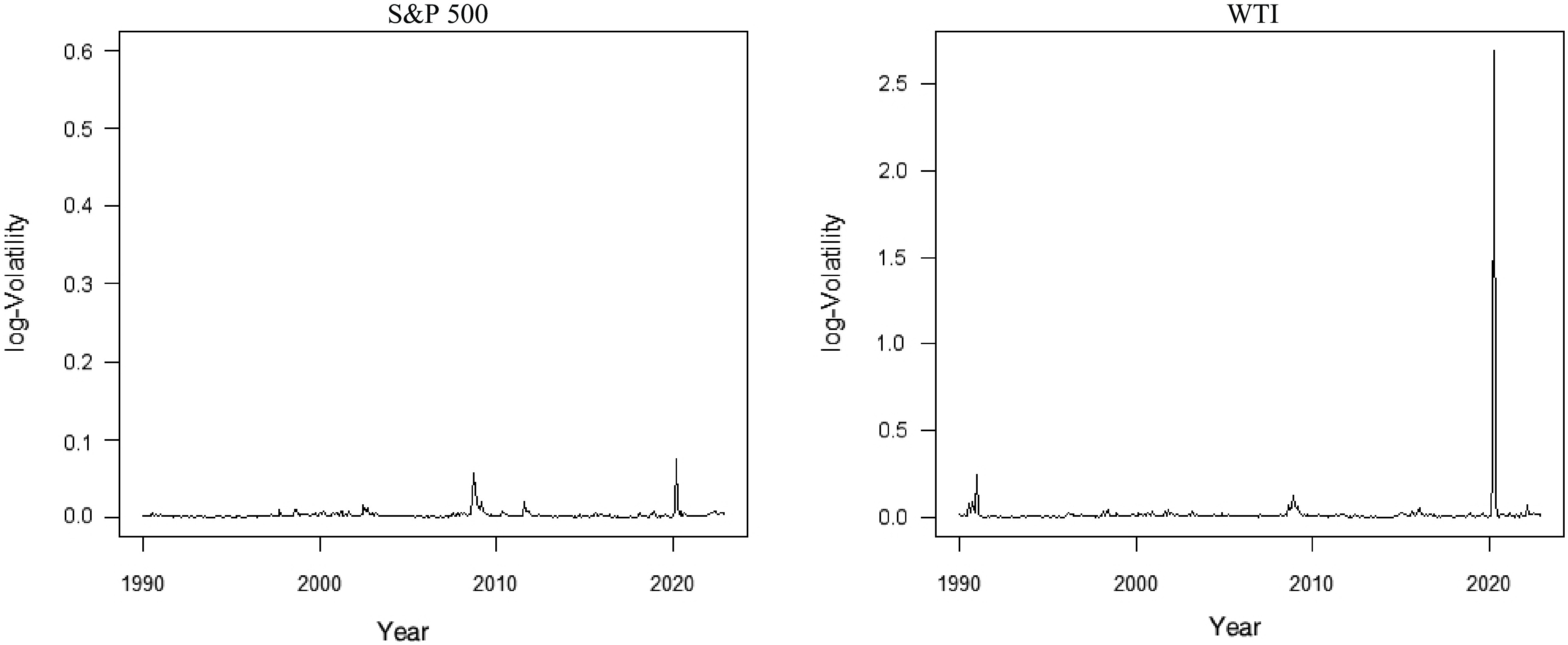
Figure 1. 

Realized volatility of oil prices and the S&P 500 index from 1990 to 2022.

To better understand the characteristics of the dataset, descriptive statistics are calculated for the prices, returns, and realized volatilities of the stock and oil markets during the sample period. As shown in Table 2, the average realized volatilities for oil and stocks are 0.019 and 0.003, respectively, with standard deviations of 0.136 and 0.006. Meanwhile, the high skewness and kurtosis values denote a leptokurtic distribution for the volatility derived from Eq. (1). The descriptive statistics also reveal marked leptokurtic characteristics in the return distributions of both equity and oil markets. The augmented Dickey–Fuller (ADF) tests suggest that the volatility series of both markets are stationary. In order to mitigate the effect of leptokurticity, we adopt the approach proposed by Paye^[47] and Wang et al.^[46], utilizing the natural logarithm of realized volatility. Consequently, the mean reversion model may be used to model and forecast volatility.

The Pearson's correlation coefficient between the volatility of the oil and stock markets is 0.5463, indicating a high correlation between the two. Concurrently, a standard linear Granger causality test is conducted between the two, based on the model detailed in Eq. (3). The Wald statistic for the null hypothesis that oil volatility does not cause stock volatility is 1.4892, with a p-value of 0.2231. Therefore, the results of the linear causality test indicate that the null hypothesis, which states that oil volatility cannot be used to forecast stock volatility, cannot be rejected. Nevertheless, the Wald statistic for the null hypothesis that stock fluctuations do not cause oil fluctuations is 10.144, with a p-value of 0.0015. This implies that it is reasonable to utilize stock volatility as a predictor of oil volatility.

In-sample performance

The entire sample is divided into two distinct periods for analysis: The in-sample and the out-of-sample periods. The in-sample estimation period, spanning from January 1990 to December 2010, is used to assess the in-sample performance of the models specified in Eqs (3), (4), and (5). The remaining period is designated for the out-of-sample evaluation period. Tables 3 and 4 present the computed coefficients for the diverse regression models alongside the t-statistics derived from the Newey–West estimator, which corrects for both heteroskedasticity and serial correlation. Furthermore, they exhibit the enhancement in the R² values (displayed as percentage increments) for each model when compared with the baseline AR(p) model specified in Eq. (2).

In different states of stock market volatility, the estimated coefficients of the TAR(p) and BAR(p) models have different performances. When the stock market is in a state of normal (low) volatility, TAR(p) and BAR(p) have fewer significant lagged volatility terms, and the persistence of oil volatility is lower. In the context of extreme (high) volatility in the stock market, the TAR(p) and BAR(p) models exhibit greater significance in their lagged volatility terms, and the persistence of oil volatility is increased. This indicates that utilizing stock volatility as a threshold effect is an effective approach for forecasting oil volatility.

Table 3 presents the within-sample estimation results of forecasting models for monthly oil volatility. The benchmark AR(6) model in Eq. (2) is compared with the extended ARX(6) specification from Eq. (3), which incorporates stock market volatility as an additional predictor ($ \beta $). Furthermore, the table reports the results of the TAR(6) model from Eq. (4), which divides the sample into two regimes depending on whether the stock market volatility $ {V}_{t,stock} $ falls below or exceeds the estimated threshold of –6.999. All models are estimated with a maximum lag order of six.

Table 4 presents the within-sample estimation results of forecasting regressions for monthly oil volatility when incorporating stock market volatility. Three specifications are considered: the benchmark AR(6) model in Eq. (2), the ARX(6) model in Eq. (3) that augments the benchmark with stock market volatility as an additional predictor, and the BAR(6) model in Eq. (5), which introduces a buffered threshold mechanism. All models are estimated with a maximum lag order of six.

The sample of oil and stock data from 1990 to 2010 is used to calculate the value of $ \text{2Λ(}\tilde{V}) $. The logarithmic likelihood values of the BAR and TAR models are 8,593.323 and 8,582.697, respectively. The final value of $ \text{2Λ(}\tilde{V}) $ is 21.252, which is much greater than the $ \chi _{1}^{2}(0.95) $ (equal to 3.841). Therefore, the null hypothesis is rejected, and we conclude that the BAR model outperforms the TAR model significantly for this sample.

Out-of-sample performance

After evaluating the in-sample performance of each model, we assess their out-of-sample forecast performance over the sample period. Forecasts of monthly crude oil volatility, incorporating stock market volatility, are generated using the recursive and rolling window estimation methods. We consider three models: ARX(p) in Eq. (3), TAR(p) in Eq. (4), and BAR(p) in Eq. (5), with the lag order p = 6. Table 5 reports the out-of-sample $ \Delta R_{oss}^{2} $ values and the corresponding Clark–West (CW) test p-values across multiple sample periods.

Table 5 reveals the following. First, based on the recursive window estimation method, the positive value of $ \Delta R_{oss}^{2} $ indicates that the TAR(p) model and the BAR(p) model have significantly better forecasting performance than the reference model AR(p) during the out-of-sample period from 2011 to 2022. The use of stock volatility as a threshold variable has been demonstrated to result in a reduction in MSPE of 6.319% and 8.176%. The p-values of the CW test are $ 6.76{\mathrm{e}}^{-4} $ and $ 3.71{\mathrm{e}}^{-4} $, respectively. The $ \Delta R_{oss}^{2} $ and p-values for the CW test results for the remaining subcycles exhibit similar values to those observed in the 2011–2022 period. This shows that the TAR(p) and BAR(p) models are markedly superior to the reference model AR(p) over various periods when stock volatility is used as the threshold variable.

Second, the forecasting capacity of ARX(p), which relies on stock volatility as a direct predictor, proves weak. It only marginally surpasses the baseline AR(p) model from 2013 to 2022, failing to surpass it during other periods. Consequently, ARX(p) in this model does not appreciably improve the precision of oil volatility forecasts when stock volatility serves as the forecasting variable.

Third, BAR(p) outperforms the TAR(p) model in terms of forecasting performance in all periods, whether based on the recursive or rolling window estimation method. When using stock volatility as a threshold variable, the BAR(p) model reduces the MSPE by approximately 2% more than the TAR(p) model. We can infer that the BAR(p) model may have better forecasting performance than the TAR(p) model in various time periods.

Fourth, the rolling window estimation method yielded similar forecasting performance for each model to that obtained by the recursive window estimation method. Nevertheless, the forecasting performance of the rolling window estimation method is slightly inferior to that of the recursive window estimation method.

Generally, fluctuations in the stock market can provide valuable information for forecasting oil fluctuations. The TAR(p) model and BAR(p) model have stronger forecasting performance when using stock volatility as the threshold variable compared with models that directly add stock volatility to the linear regression in Eq. (3). By contrast, neither the linear regression models nor the reference autoregressive models that use stock information as a predictor demonstrate an advantage. Furthermore, the results show that the BAR(p) model outperforms the TAR(p) model in terms of forecasting performance. This suggests that the hysteresis effect considered in this study can provide more valuable information for forecasting oil volatility.

Selecting the appropriate lag order p for autoregressive models requires a formal and systematic approach to avoid over-parameterization while capturing sufficient historical information. Although our baseline analysis uses p = 6 according to established literature^[47,46], a systematic sensitivity analysis is essential. Guided by the AIC framework, which mathematically penalizes the inclusion of excessive parameters k as the lag order p increases, we expanded our empirical evaluation. To ensure the robustness of the TAR(p) and BAR(p) models, we investigated whether the forecasting superiority of the BAR framework holds under nearby lag structures (p = 5 and p = 7) that also yield competitive AIC scores.

Tables 6 and 7 present the evaluation results of each model under different lag orders (p = 5 and p = 7). The models include the ARX(p) model with stock volatility as an exogenous variable, as well as the TAR(p) and BAR(p) models with stock volatility as a threshold variable. The results are based on the recursive and rolling window estimation methods.

The results of forecasting monthly crude oil volatility incorporating stock volatility are obtained using recursive and rolling window regression estimation methods. The models include an ARX(p) model as specified in Eq. (3), a TAR(p) model as shown in Eq. (4), and a BAR(p) model as shown in Eq. (5), with the lag order set to 5 or to 7.

First, the recursive window estimation method shows that the TAR(5) model and BAR(5) model, with stock volatility as the threshold variable, can reduce the MSPE from 6.263% to 10.944% and 6.994% to 11.697%, respectively, in comparison with the reference model, namely AR(5). The rolling window estimation method suggests that the TAR(5) and BAR(5) models can reduce MSPE from 5.629% to 9.807% and from 6.532% to 11.191%, respectively, compared with the AR(5) reference model. Meanwhile, the p-values of the CW test for the TAR(5) and BAR(5) models are both less than 0.1. The results in Table 7 are consistent with those in Table 6, suggesting that both the TAR(p) and BAR(p) models outperform the ARX(p) model of Eq. (3).

Second, regardless of whether the recursive or rolling window estimation method is used in every period, the BAR(p) model outperforms the TAR(p) model in terms of forecasting performance. When using stock volatility as a threshold variable, the BAR(p) model reduces the MSPE by approximately 1.5% more than the TAR(p) model.

Third, Tables 6 and 7 show that the BAR(p) and TAR(p) models, using stock volatility as the threshold variable, outperform the ARX(p) model in terms of forecasting performance. At the same time, the BAR(p) model outperforms the TAR(p) model in all periods in terms of forecast accuracy, as shown in Tables 5–7. This indicates the robustness of both models for lag-order selection.

Overall, the evaluation results for the forecast performance of the BAR(p) and TAR(p) models with stock volatility as the threshold variable are similar, despite slight differences, when selecting different lag orders. This indicates that the forecasting of both models is robust to the selection of the lagged order.

This study explores the effect of stock market volatility on the nonlinear threshold of the oil market using the BAR model. The results, for both in-sample and out-of-sample periods, demonstrate the value of the stock volatility threshold effect for forecasting oil volatility. According to the in-sample results, the BAR model, which takes stock volatility as the threshold variable, shows better fitting results than the TAR model, the ARX model, and the reference model. In terms of both the out-of-sample $ \Delta R_{oss}^{2} $ and CW^[50] statistics, the BAR model demonstrates a forecasting advantage over models such as the TAR model when stock volatility is used as the threshold variable. This indicates that stock volatility has a threshold effect on oil volatility forecasts. Additionally, the BAR model is robust when selecting the model's lag order.

Meanwhile, our empirical results demonstrate the existence of a hysteresis threshold effect in stock volatility for oil volatility forecasts. The BAR model is more effective than the linear regression model and the TAR model for extracting stock volatility information for oil volatility forecasts. This study could help investors adjust their investment portfolios to reduce risks as well as help governments formulate reasonable economic policies to balance fluctuations in the market.

Finally, we acknowledge certain limitations in our study that provide avenues for future research. The empirical comparison in this paper is deliberately restricted to a set of closely related autoregressive benchmark models (AR, ARX, and TAR) to isolate and verify the effectiveness of the hysteresis effect. Consequently, although the BAR model demonstrates a clear advantage within this specific family of models, this study does not establish its broader superiority in the general oil volatility forecasting literature. Future studies should expand the benchmark set to include GARCH-type models, MSM, and advanced machine-learning-based approaches to comprehensively evaluate the absolute forecasting power of the BAR model in more complex forecasting scenarios.