-
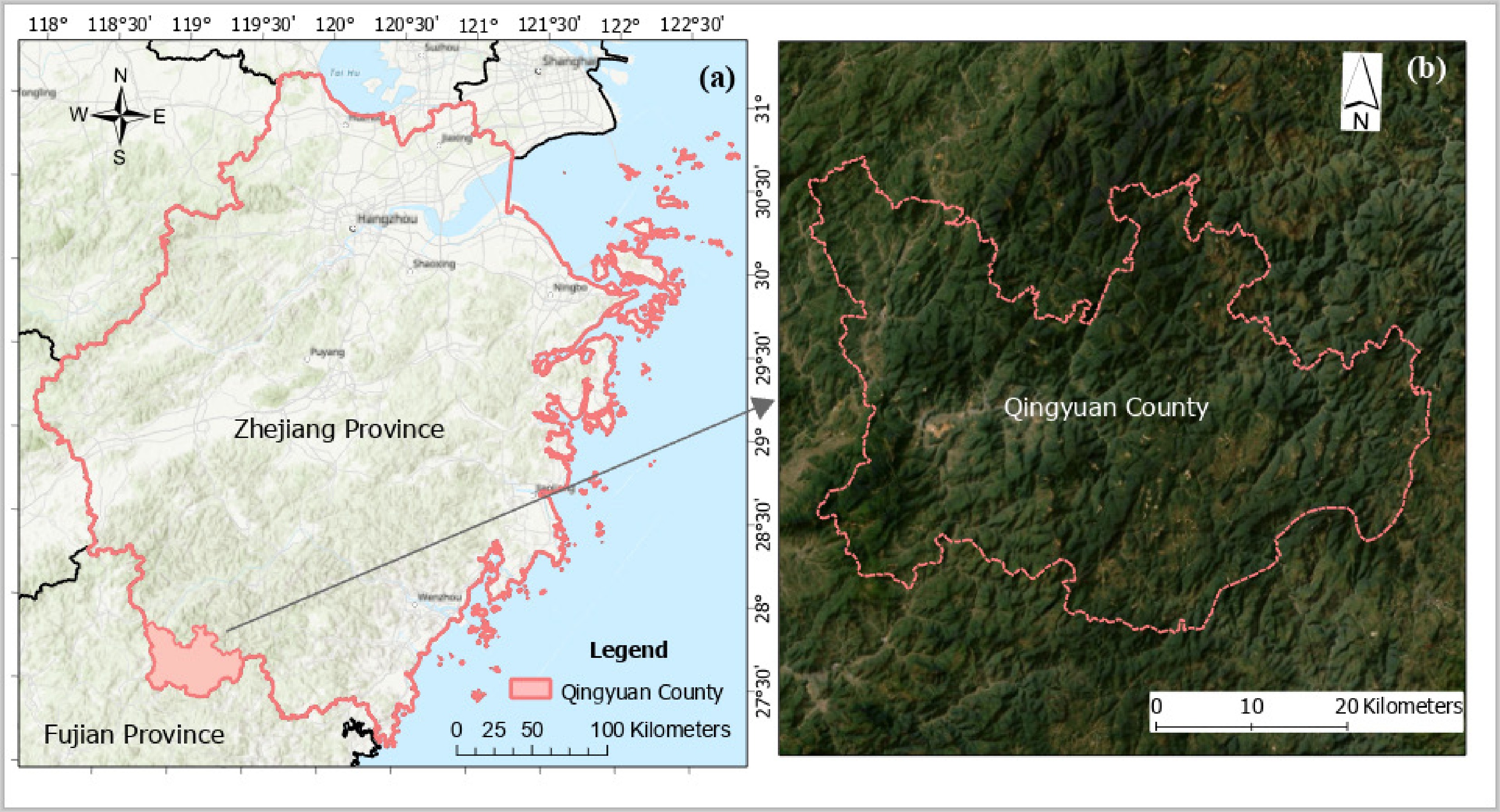
Figure 1.
Study area map of Qingyuan County, Zhejiang Province. The map is from the 2019 Chinese administrative division vector map (
https://download.csdn.net/download/gognzixiaobai666/14033998 ). (a) represents the vector map of Zhejiang Province, and (b) is the topographic map of Qingyuan County. -
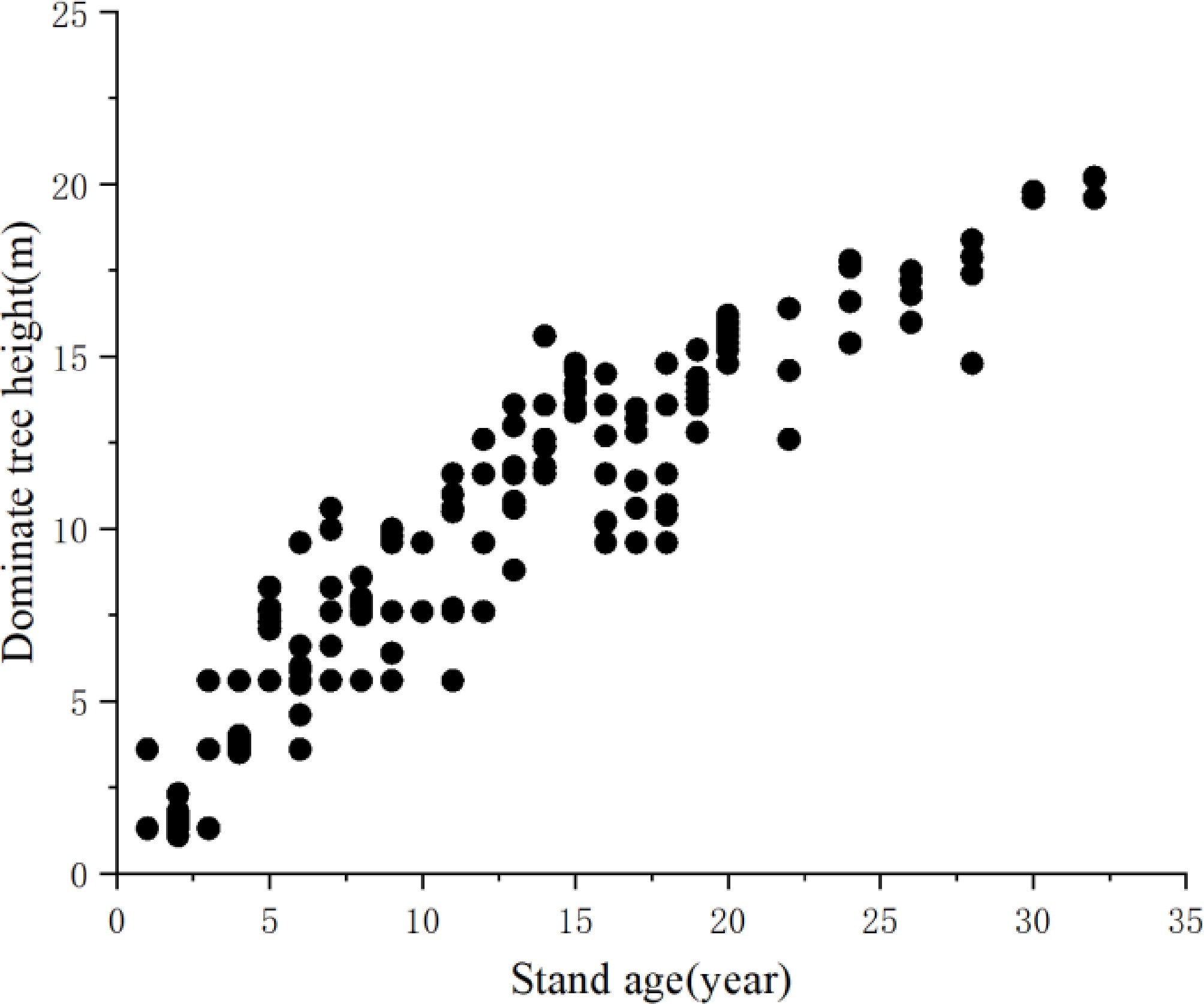
Figure 2.
Stem analysis data of Chinese fir.
-
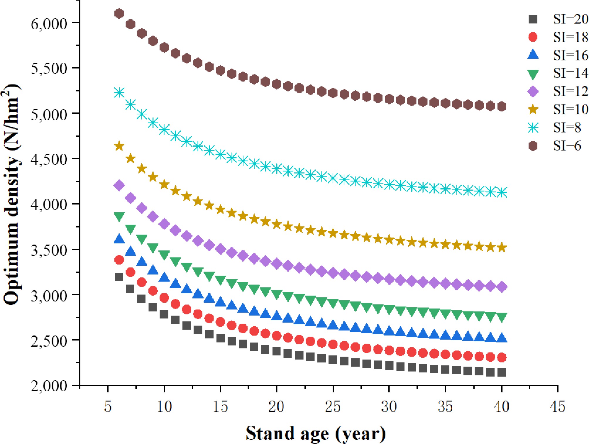
Figure 3.
Optimum stand density under different age and site index.
-
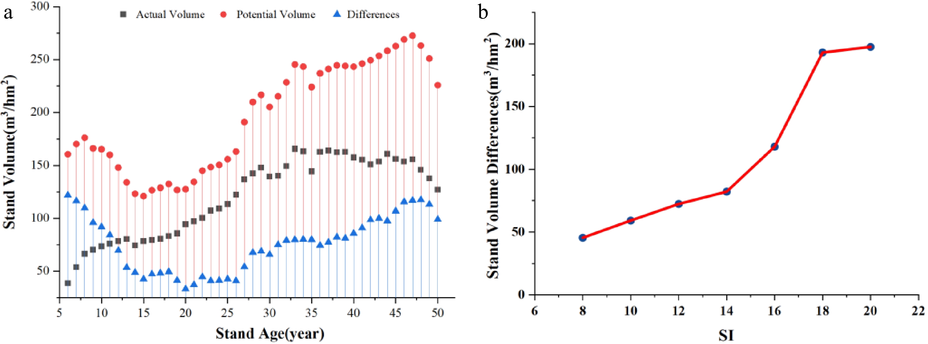
Figure 4.
Comparison of stand potential volume and actual volume at different ages and densities. (a) represents comparison of stand potential volume and actual volume at different ages, (b) represents comparison of stand potential volume and actual volume at different densities.
-
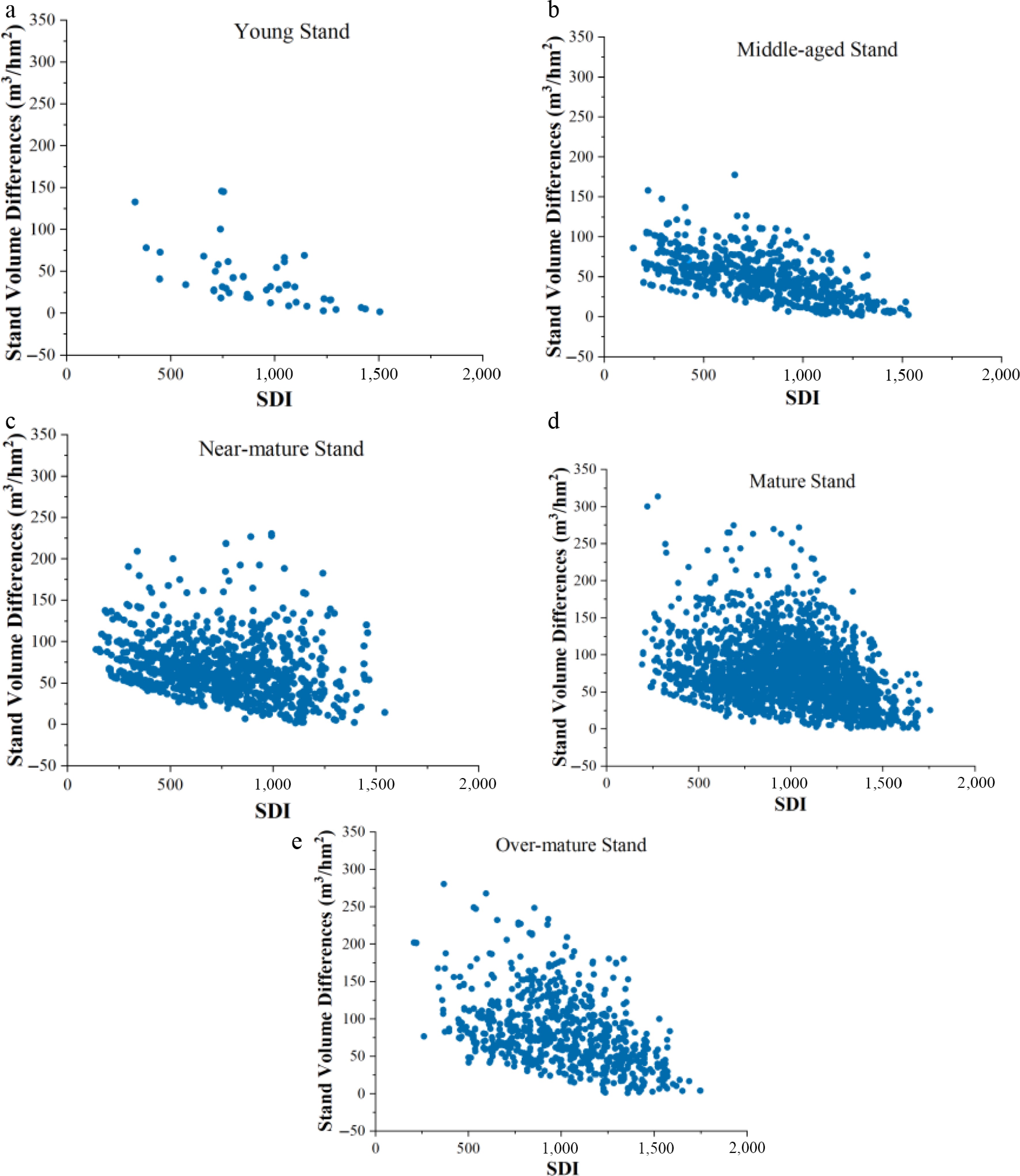
Figure 5.
Difference between potential and actual volume of stands under different SDI. (a) represents young stand, (b) represents middle-aged stand, (c) represents near-mature stand, (d) represents mature stand, (e) represents over-mature stand.
-
Variables Fitting data Testing data Minimum
valueMaximum
valueMean
valueStandard
deviationMinimum
valueMaximum
valueMean
valueStandard
deviationStand age (year) 6 46 18.2 7.57 6 43 19.4 7.83 Density (N/hm2) 750 4,800 2,125 654.32 1,200 4,500 2,358 633.24 Average tree height (H, m) 4.3 21.5 12.0 3.71 4.4 22.0 12.1 4.13 Dominant tree height (HT, m) 5.1 23.5 13.7 3.60 5.0 23.2 13.8 3.11 Volume (m3 /ha) 11.3 432.3 100.8 75.9 11.7 429.0 100.9 76.1 Table 1.
Subcompartments data for model fitting and testing.
-
Variables Fitting data Testing data Minimum
valueMaximum
valueMean
valueStandard
deviationMinimum
valueMaximum
valueMean
valueStandard
deviationAge (t) 1 32 11.8 7.2 1 32 11.7 7.2 Dominant tree height (HT, m) 1.1 20.6 9.7 4.1 1.3 20.2 9.6 4.2 Table 2.
Stem analysis data for model fitting and testing.
-
Model no. Theoretical equations Elimination parameters Initial solution for $ {X}_{0} $ Difference equations M1 Modified Weibull: $ {h} ={a}\left(1-{e}^{{{-bt}^{c}}}\right) $ $ a={e}^{{{X}_{0}}} $ $ c={c}_{1}+{c}_{2}{X}_{0} $ $ {X}_{0}=\ln {h}_{1}-\ln \left(1-{e}^{{{{{-bt}_{1}}}^{{{c}_{1}}+{{c}_{2}}{{X}_{0}}}}}\right) $ $ {h}_{2}={e}^{{{X}_{0}}}\left(1-{e}^{{{{{-bt}_{2}}}^{{{c}_{1}}+{{c}_{2}}{{X}_{0}}}}}\right) $ M2 $ a={e}^{{{X}_{0}}} $ $ c={c}_{1}+{c}_{2}/{X}_{0} $ $ {X}_{0}=\ln {h}_{1}-\ln \left(1-{e}^{{{{{-bt}_{1}}}^{{{c}_{1}}+{{c}_{2}}/{{X}_{0}}}}}\right) $ $ {h}_{2}={e}^{{{X}_{0}}}\left(1-{e}^{{{{{-bt}_{2}}}^{{{c}_{1}}+{{c}_{2}}/{{X}_{0}}}}}\right) $ M3 Korf: $ {h} ={a}{e}^{{{-bt}^{-c}}} $ $ a={e}^{{{X}_{0}}} $ $ c={c}_{1}+{c}_{2}{X}_{0} $ $ {X}_{0}=\ln {h}_{1}+b{t}^{-\left({c}_{1}+{c}_{2}{X}_{0}\right)} $ $ {h}_{2}={e}^{{{X}_{0}}}{e}^{{{{{-bt}_{2}}}^{-\left({c}_{1}+{c}_{2}{X}_{0}\right)}}} $ $ {h}_{2}={e}^{{{X}_{0}}}{e}^{{{{{-bt}_{2}}}^{-\left({c}_{1}+{c}_{2}/{X}_{0}\right)}}} $ M4 $ a={e}^{{{X}_{0}}} $ $ c={c}_{1}+{c}_{2}/{X}_{0} $ $ {X}_{0}=\ln {h}_{1}+b{t}^{-\left({c}_{1}+{c}_{2}/{X}_{0}\right)} $ $ {h}_{2}={e}^{{{X}_{0}}}{e}^{{{{{-bt}_{2}}}^{-\left({c}_{1}+{c}_{2}/{X}_{0}\right)}}} $ M5 Richards: $ {h} = {a}{\left(1-{e}^{-bt}\right)}^{c} $ $ a={e}^{{{X}_{0}}} $ $ \text{c=}{c}_{1}+{c}_{2}{X}_{0} $ $ {X}_{0}=\left(\ln {h}_{1}-{c}_{1}{F}_{0}\right)/\left(1+{c}_{2}{F}_{0}\right) $ $ {F}_{0}=\ln \left(1-{e}^{{{-bt}_{1}}}\right) $ $ {h}_{2}={e}^{{{X}_{0}}}{\left(1-{e}^{{{-bt}_{2}}}\right)}^{{{c}_{1}}+{{c}_{2}}{{X}_{0}}} $ M6 $ a={e}^{{{X}_{0}}} $ $ c={c}_{1}+{c}_{2}/{X}_{0} $ $ {X}_{0}=\dfrac{1}{2}\left[{F}_{0}+\sqrt{{{{F}_{0}}}^{2}-4\times {c}_{2}\ln \left(1-{e}^{{{-bt}_{1}}}\right)}\right] $ $ {F}_{0}={\ln {h}_{1}-c}_{1}\ln \left(1-{e}^{{{-bt}_{1}}}\right) $ $ {h}_{2}={e}^{{{X}_{0}}}{\left(1-{e}^{{{-bt}_{2}}}\right)}^{{{c}_{1}}+{{c}_{2}}/{{X}_{0}}} $ Note: $ {h}_{1} $ $ {h}_{2} $ $ {t}_{1} $ $ {t}_{2} $ Table 3.
Different site index equations.
-
Model Parameter value Fitting index Testing index a11 b11 a12 b12 R2 RMSE MAE Density effect model 1.06E-4 2.724 2.407E-9 3.393 0.839 28.104 20.602 Table 4.
Fitting and testing results of the density effect model.
-
Model no. Parameters Estimated value Standard error Significance testing (p) R2 RMSE MAE M1 b 0.410 0.123 0.002** 0.998 0.343 0.259 $ {c}_{1} $ 1.471 0.162 < 0.001*** $ {c}_{2} $ −0.395 0.052 < 0.001*** M2 b 0.403 0.104 < 0.001*** 0.999 0.261 0.257 $ {c}_{1} $ −0.580 0.199 0.006** $ {c}_{2} $ 2.671 0.401 < 0.001*** M3 b 1.583 0.568 0.008** 0.982 1.336 0.409 $ {c}_{1} $ 2.803 622,600 0.999 $ {c}_{2} $ 2.799 403,800 0.999 M4 b 1.074 0.408 0.013* 0.999 0.101 0.232 $ {c}_{1} $ −0.156 0.248 0.533 $ {c}_{2} $ 1.881 0.556 0.001** M5 b 0.053 0.014 < 0.001*** 0.969 1.778 0.400 $ {c}_{1} $ −0.174 0.047 < 0.001*** $ {c}_{2} $ 0.222 0.049 < 0.001*** M6 b 0.072 0.026 0.009** 0.606 6.371 0.631 $ {c}_{1} $ 1.865 1.025 0.078 $ {c}_{2} $ −1.763 2.806 0.534 Note: * p < 0.05; ** p < 0.01; *** p < 0.001. Table 5.
Parameter estimates and fitting and testing indicators of site index equations.
-
Stand age Optimal density SI = 20 SI = 18 SI = 16 SI = 14 SI = 12 SI = 10 SI = 8 SI = 6 6 3,195 3,382 3,602 3,870 4,204 4,637 5,227 6,099 7 3,061 3,246 3,466 3,733 4,067 4,501 5,096 5,980 8 2,951 3,135 3,353 3,620 3,954 4,389 4,988 5,881 9 2,859 3,042 3,260 3,525 3,859 4,295 4,896 5,797 10 2,782 2,963 3,180 3,445 3,778 4,214 4,817 5,724 11 2,715 2,895 3,111 3,375 3,708 4,144 4,749 5,660 12 2,657 2,836 3,051 3,314 3,647 4,083 4,689 5,605 13 2,606 2,784 2,998 3,261 3,593 4,029 4,636 5,555 14 2,560 2,738 2,951 3,213 3,544 3,981 4,588 5,511 15 2,520 2,697 2,909 3,171 3,502 3,938 4,546 5,471 16 2,484 2,660 2,872 3,133 3,463 3,899 4,508 5,435 17 2,452 2,627 2,838 3,098 3,428 3,864 4,473 5,402 18 2,422 2,597 2,808 3,067 3,396 3,832 4,442 5,373 19 2,396 2,570 2,780 3,039 3,368 3,803 4,413 5,346 20 2,371 2,545 2,755 3,013 3,341 3,776 4,387 5,321 21 2,349 2,523 2,732 2,989 3,317 3,752 4,362 5,298 22 2,329 2,502 2,710 2,968 3,295 3,730 4,340 5,277 23 2,310 2,483 2,691 2,948 3,275 3,709 4,320 5,258 24 2,293 2,465 2,673 2,929 3,256 3,690 4,301 5,240 25 2,277 2,449 2,656 2,912 3,239 3,673 4,284 5,223 26 2,263 2,434 2,641 2,897 3,223 3,656 4,267 5,208 27 2,249 2,420 2,627 2,882 3,208 3,641 4,252 5,194 28 2,237 2,407 2,613 2,868 3,194 3,627 4,238 5,180 29 2,225 2,395 2,601 2,856 3,181 3,614 4,225 5,168 30 2,214 2,384 2,590 2,844 3,169 3,602 4,213 5,156 31 2,204 2,374 2,579 2,833 3,158 3,591 4,202 5,146 32 2,195 2,364 2,569 2,823 3,148 3,580 4,191 5,136 33 2,186 2,355 2,560 2,814 3,138 3,570 4,182 5,126 34 2,178 2,347 2,551 2,805 3,129 3,561 4,172 5,117 35 2,170 2,339 2,543 2,796 3,121 3,553 4,164 5,109 36 2,163 2,331 2,536 2,789 3,113 3,545 4,156 5,101 37 2,156 2,324 2,528 2,781 3,105 3,537 4,148 5,094 38 2,150 2,318 2,522 2,775 3,098 3,530 4,141 5,087 39 2,144 2,312 2,516 2,768 3,092 3,523 4,134 5,081 40 2,138 2,306 2,510 2,762 3,085 3,517 4,128 5,075 Table 6.
Optimal density based on maximum stand volume yield with various sites.
Figures
(5)
Tables
(6)