-
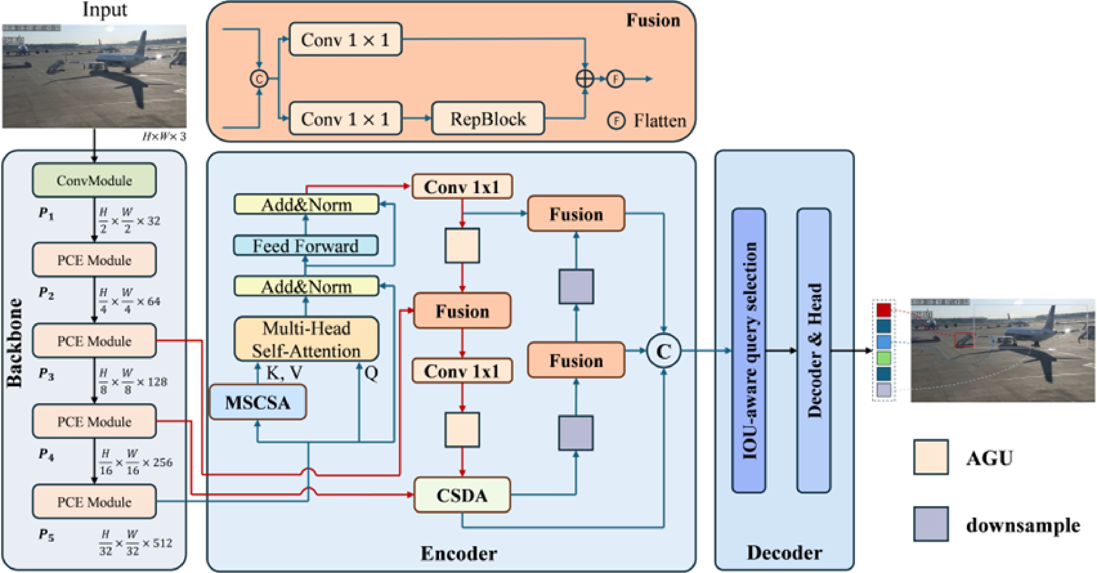
Figure 1.
Overall flow of the proposed algorithm.
-
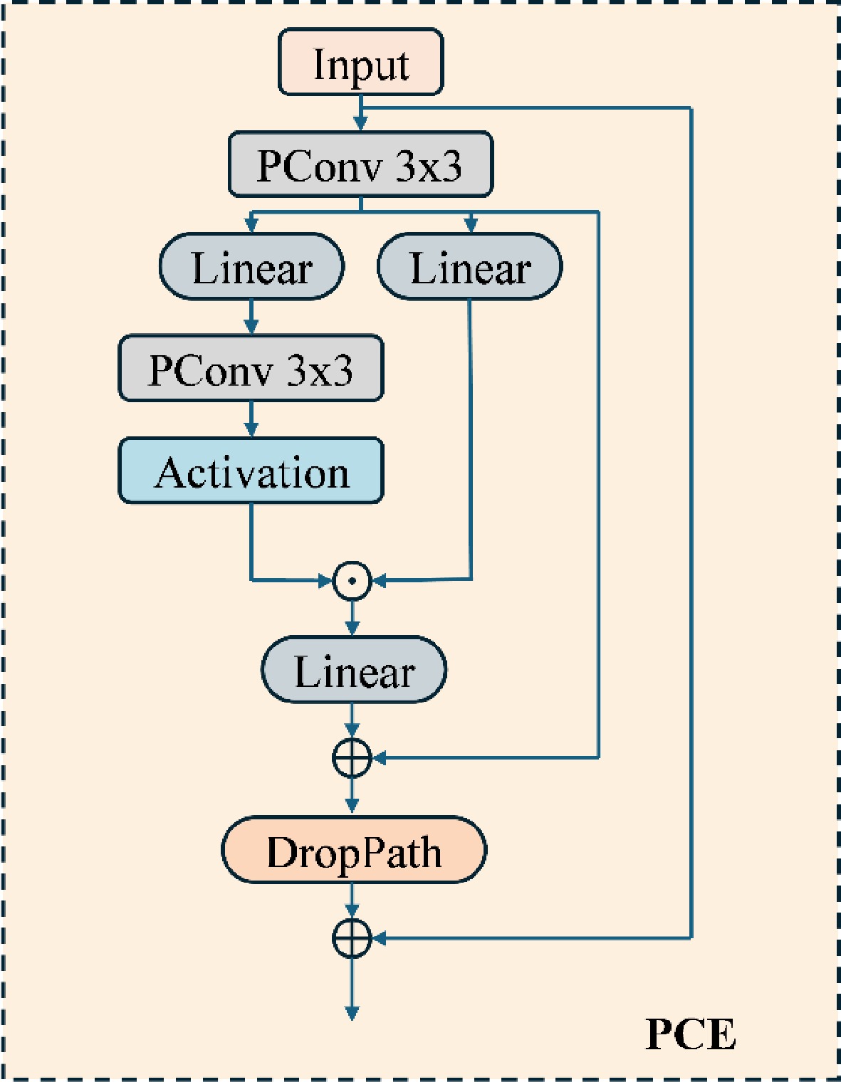
Figure 2.
PCE module.
-
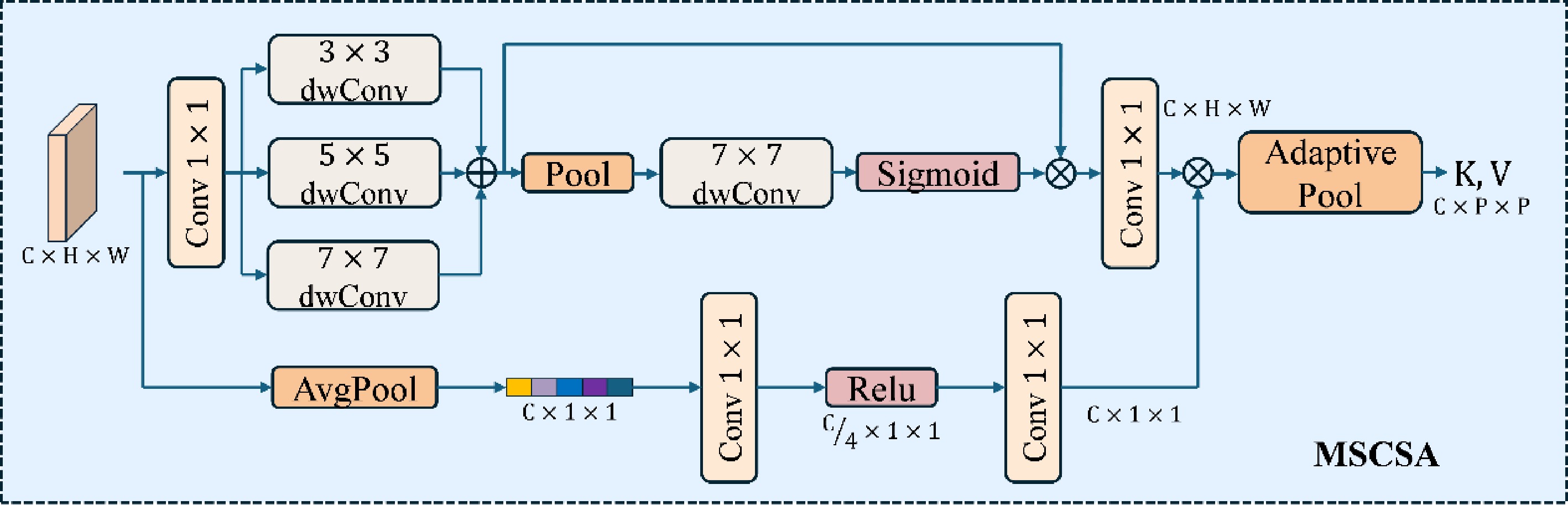
Figure 3.
MSCSA module.
-
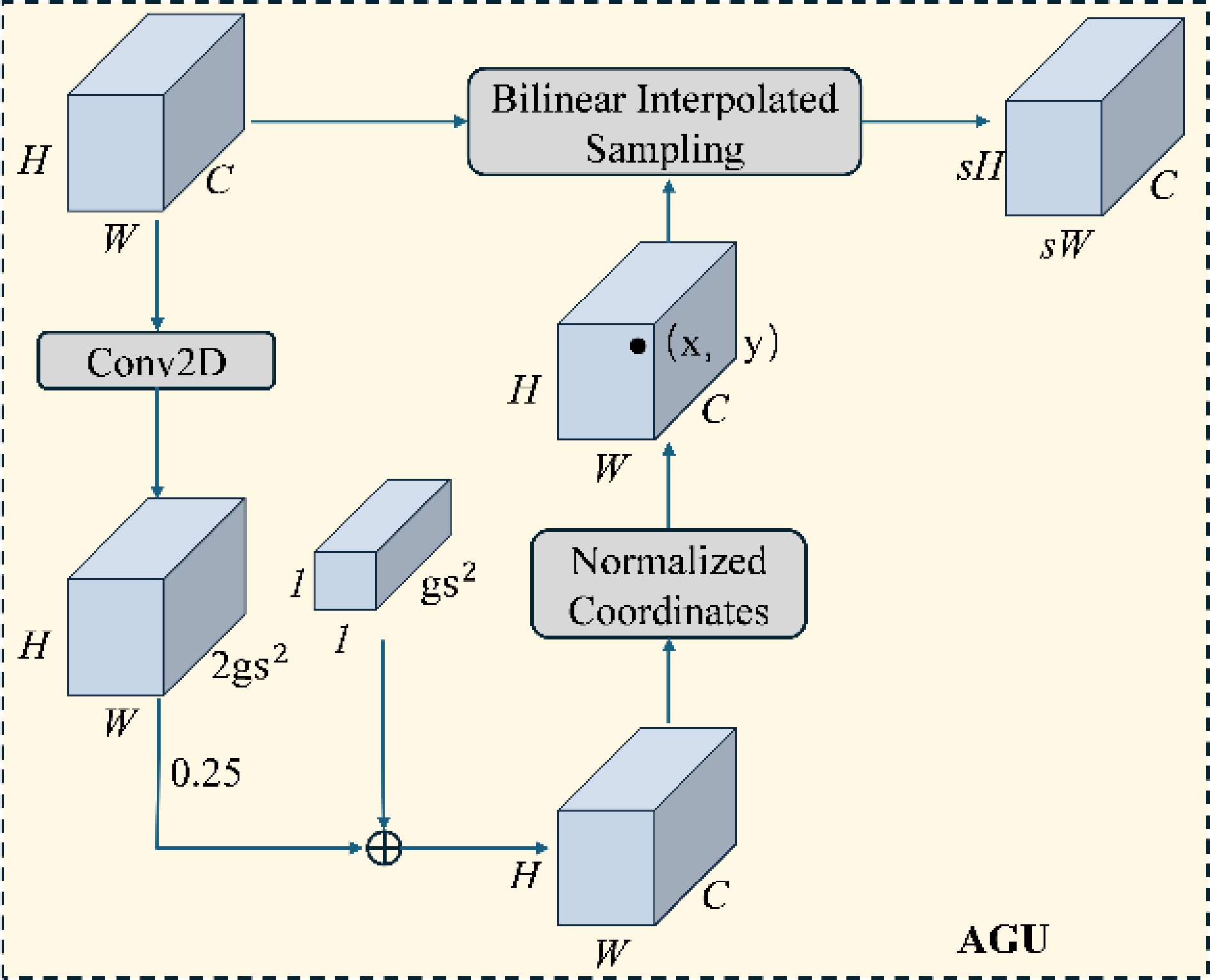
Figure 4.
AGU module.
-
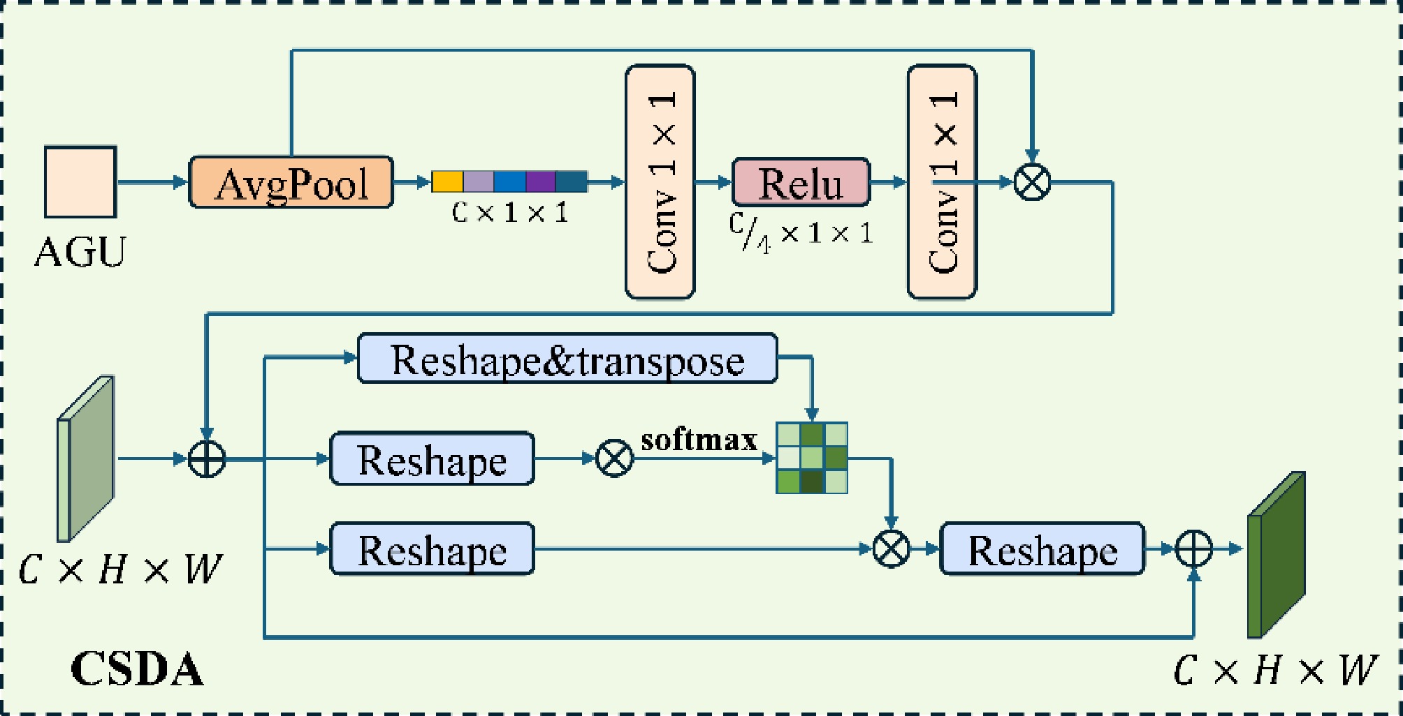
Figure 5.
CSDA module.
-
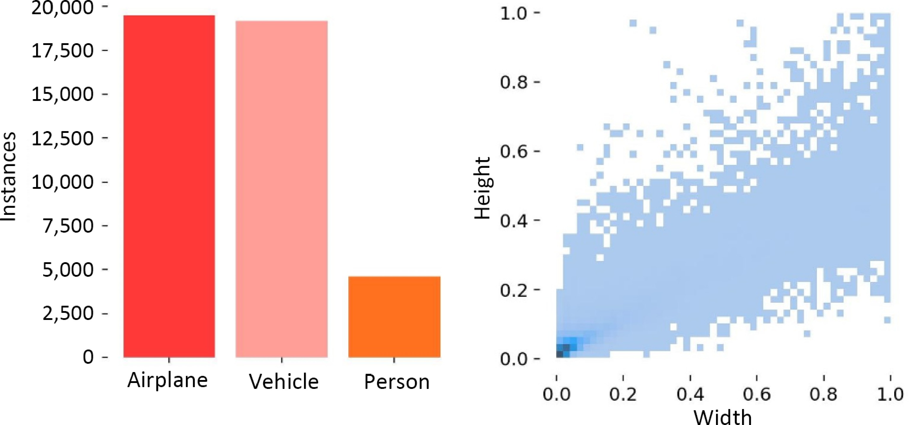
Figure 6.
Target category distribution and size diagram.
-
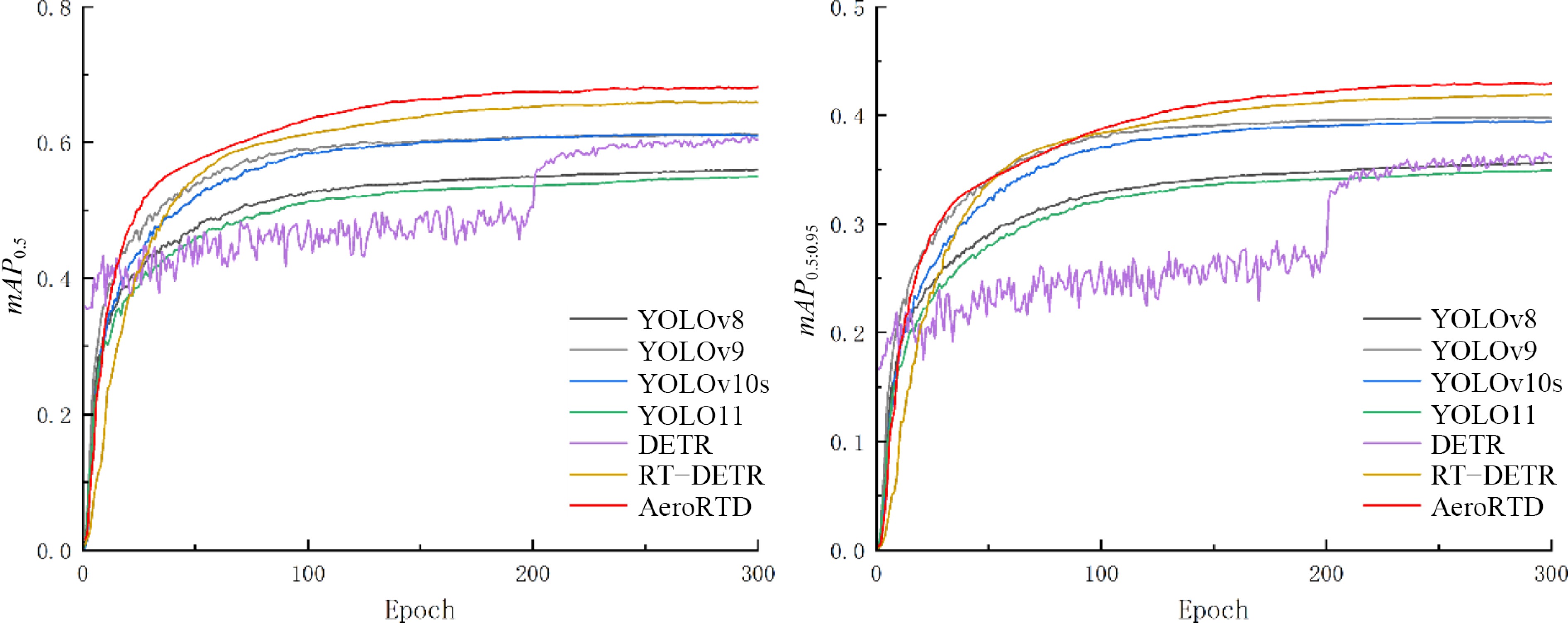
Figure 7.
Comparative experimental chart.
-
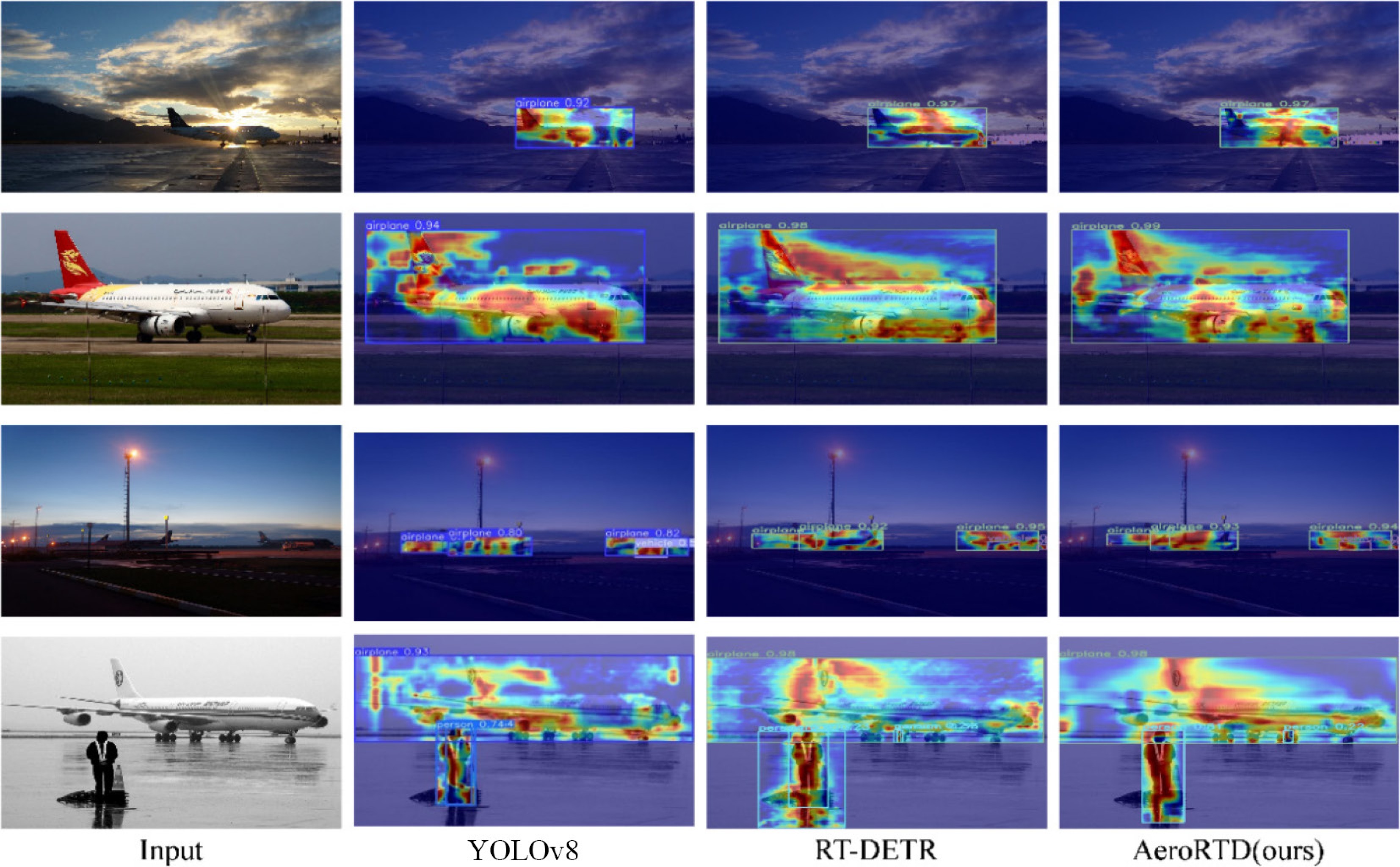
Figure 8.
Visualization results.
-
Module Targeted problem Key idea Position Unique role PCE Small objects/fine-grained features Parallel partial conv + linear fusion Backbone Enhance local details MSCSA Scale variation Multi-scale conv + self-attention Encoder Model cross-scale context AGU Misaligned upsampling Dynamic sampling grid Fusion stage Achieve precise alignment CSDA Redundant features Channel + spatial attention Fusion stage Suppress redundant information Table 1.
Functional comparison of proposed modules.
-
Parameters Settings Epochs 300 Batch 16 Imgsz 640 Workers 4 Optimizer AdamW[38] Lr0 0.0001 Table 2.
Setting table of experimental environment parameters.
-
Modules P R mAP0.5 mAP0.5:0.95 Params GFLOPs FPS YOLOv8[23] 0.701 0.518 0.56 0.357 3,006,233 8.1 13.14 YOLOv9[24] 0.743 0.567 0.613 0.399 7,168,249 26.7 10.77 YOLOv10s[25] 0.734 0.567 0.611 0.394 8,037,282 24.5 11.96 YOLOv11[39] 0.659 0.521 0.55 0.35 2,582,737 6.3 12.96 DETR[8] – – 0.604 0.362 36,739,785 100.94 11.85 RT-DETR[15] 0.754 0.612 0.659 0.419 19,875,612 56.9 22.59 AeroRTD (ours) 0.758 0.635 0.681 0.43 15,762,572 50.9 23.89 Bold values represent the best-performing results for the corresponding metrics. Table 3.
Comparison parameter table.
-
Table 4.
Performance comparison on VisDrone2019 dataset.
-
Modules P R mAP0.5 mAP0.5:0.95 Params GFLOPs FPS RT-DETR (baseline) 0.754 0.612 0.659 0.419 19,875,612 56.9 22.59 Baseline + A 0.757 0.624 0.669 0.429 15,405,804 46.2 25.47 Baseline + A + B 0.76 0.624 0.675 0.424 15,726,988 50.7 23.03 Baseline + A + B + C 0.758 0.635 0.681 0.43 15,762,572 50.9 23.89 Table 5.
Table of ablation experiments.
Figures
(8)
Tables
(5)