-
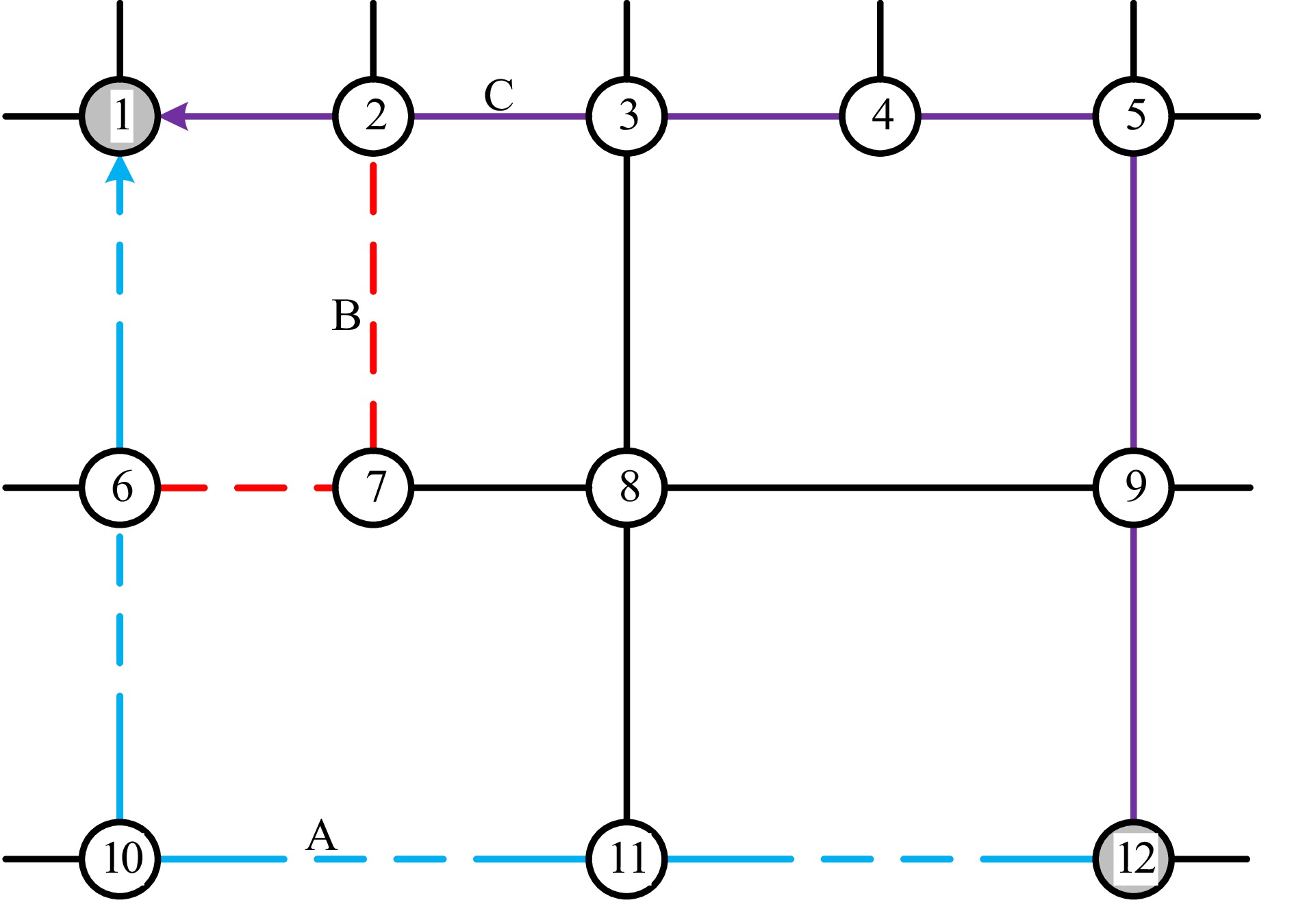
Figure 1.
MOCP-RVTO instruction on roads.
-
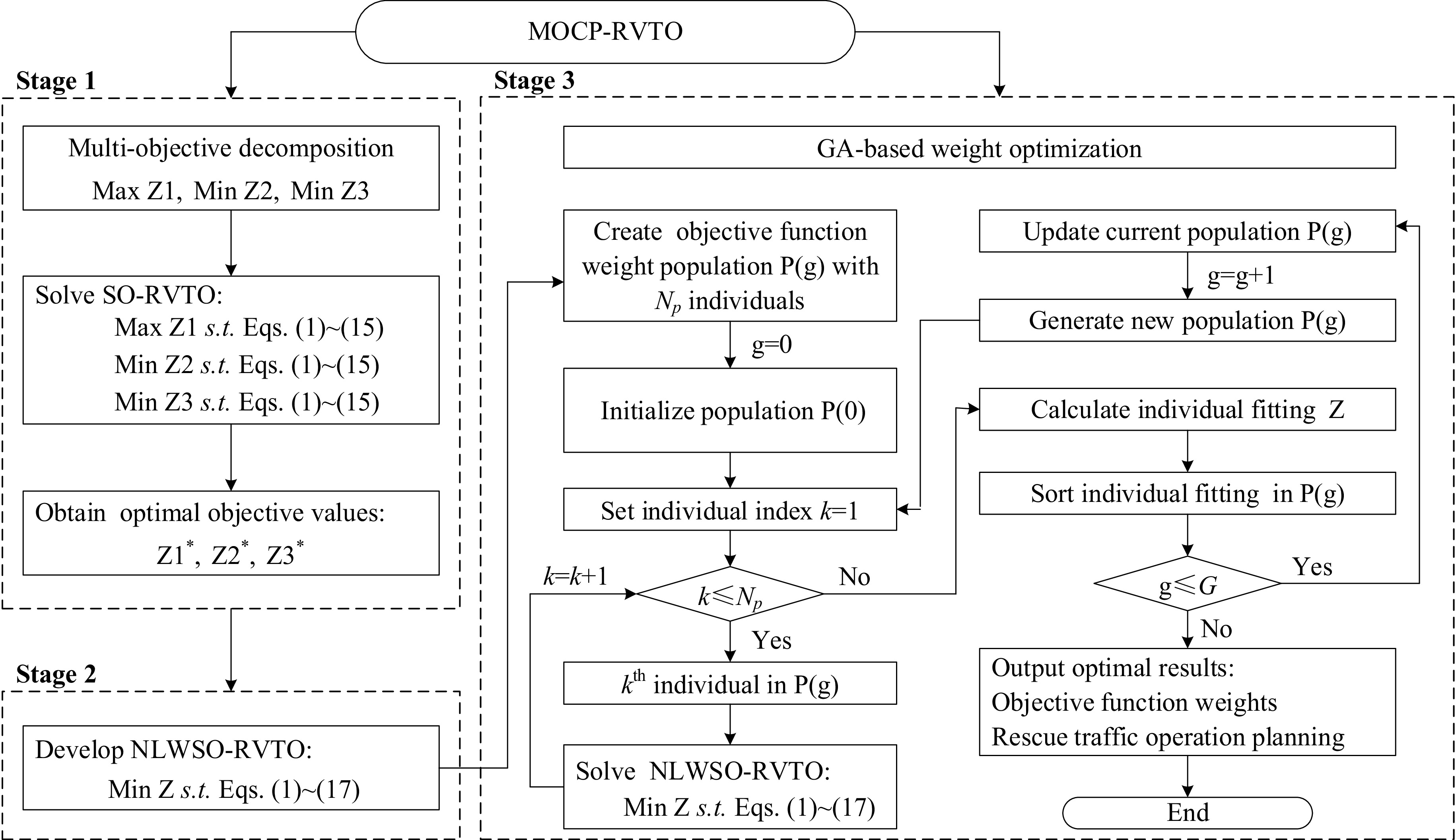
Figure 2.
GAD-based MOCP-RVTO solving approach execution flow diagram.
-
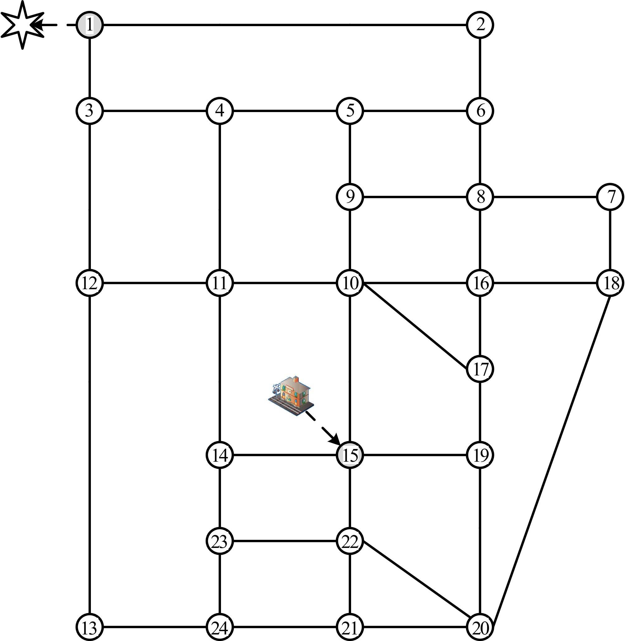
Figure 3.
Sioux Falls example network structure.
-
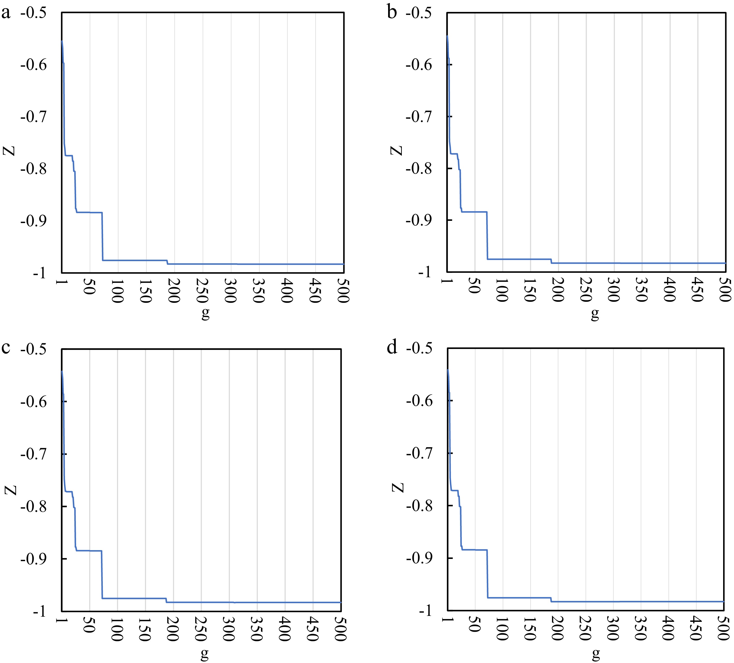
Figure 4.
Z-based fitting curves. (a) ds = 60. (b) ds = 120. (c) ds = 180. (d) ds = 240.
-
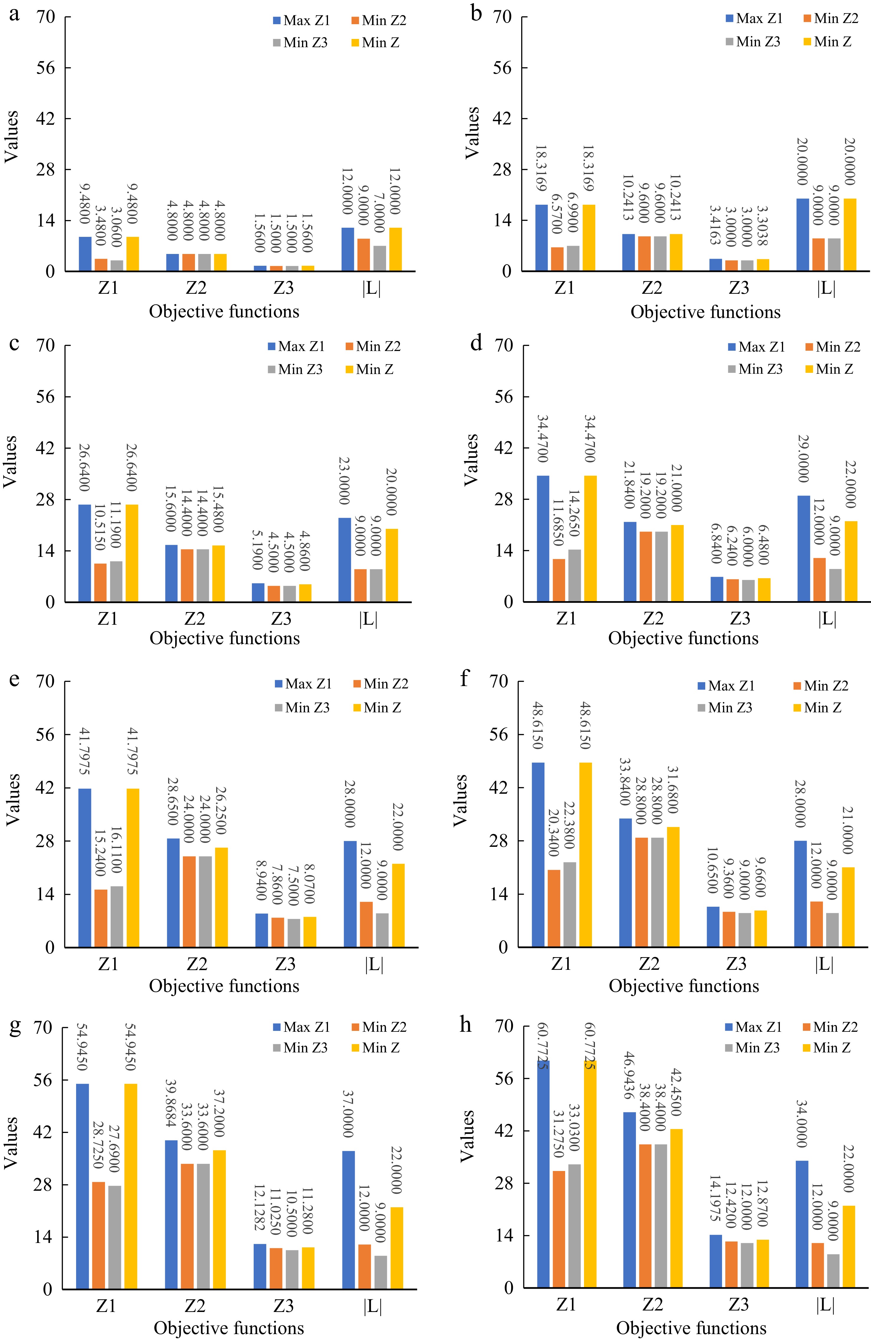
Figure 5.
Objective function values based on different optimal objectives. (a) ds = 30. (b) ds = 60. (c) ds = 90. (d) ds = 120. (e) ds = 150. (f) ds = 180. (g) ds = 210. (h) ds = 240. The unit of Z1 value is 100, the unit of Z2 value is 10,000, the unit of Z3 value is also 100, and the unit of |L| value is 1.
-
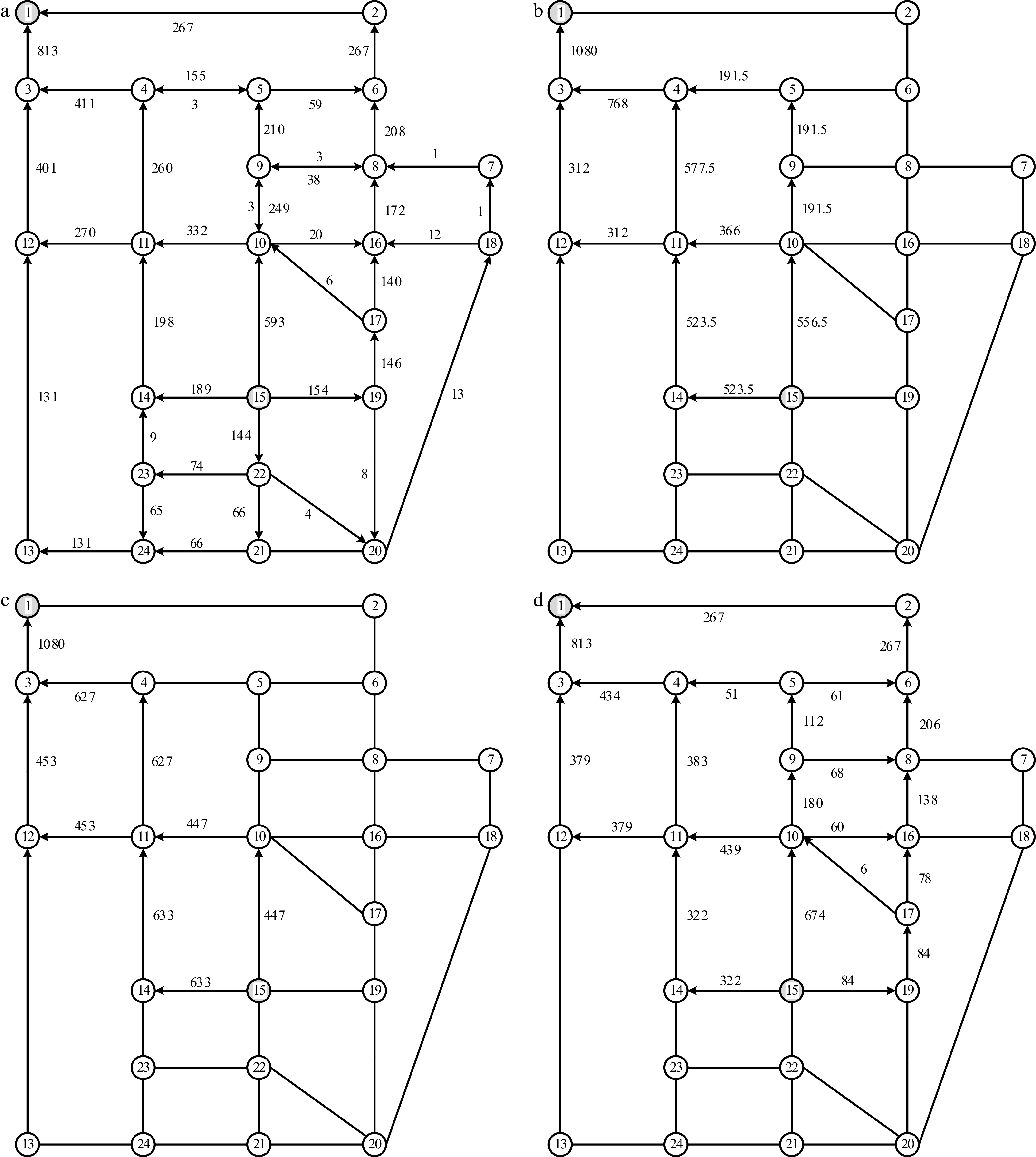
Figure 6.
Total rescue vehicle traffic volumes assigned to roads. (a) Max Z1. (b) Min Z2. (c) Min Z3. (d) Min Z.
-
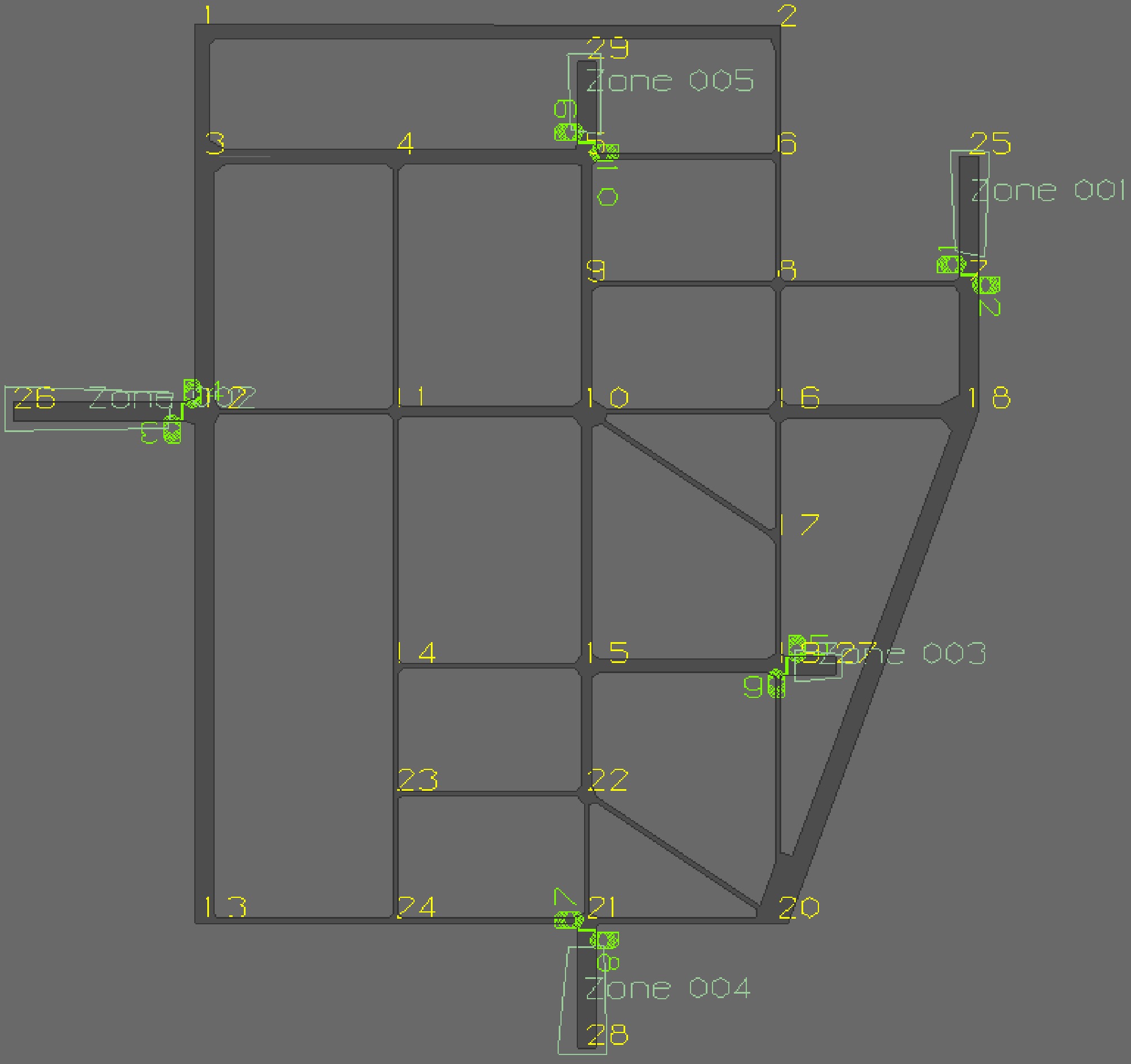
Figure 7.
Sioux Falls Paramics social vehicle traffic simulation network.
-
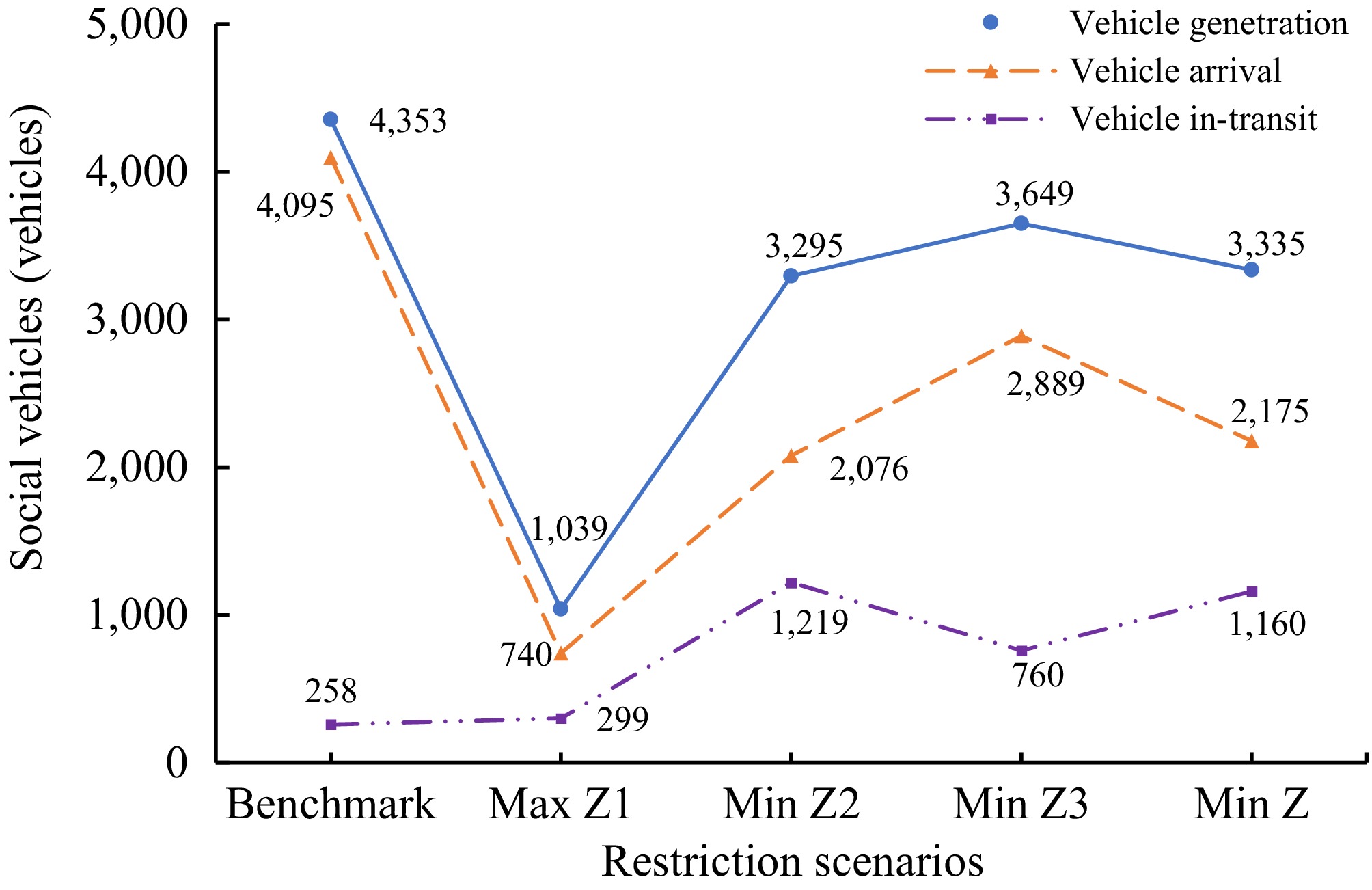
Figure 8.
Number of social vehicles.
-
Objective index Route index A B C Traffic efficiency L M H Traffic distance L M H Traffic distribution L M H H, M, and L represent the high, medium, and low levels, respectively. Table 1.
Traffic route characteristics.
-
Notations Definitions Sets $ L $ Set of links that constituting the rescue vehicle traffic network $ L' $ Set of links where rescue vehicles enter the disaster position from the road network, $ L'\subset L $ $ L'' $ Set of links where rescue vehicles enter the road network from the rescue station, $ L''\subset L $ $ S $ Set of rescue stations $ \Gamma _{i}^{+} $ Set of links that connect with link i in its downstream direction, $ i\in L,\Gamma _{i}^{+}\subset L $ $ \Gamma _{i}^{-} $ Set of links that connect with link i in its upstream direction, $ i\in L,\Gamma _{i}^{-}\subset L $ $ T $ Set of integer time periods that describe the dynamic rescue vehicle traffic network loading process Indices $ i,j $ Index of any link on the road network, $ i,j\in L $ $ t,\tau $ Index of any time period, $ t,\tau \in T $ $ s $ Index of any rescue station, $ s\in S $ $ o $ Index of the disaster position Parameters $ \alpha ,\delta $ Linear interpolation coefficient of cumulative traffic volume in non-integer time periods $ {d}_{s} $ Rescue traffic demand that represents the number of rescue vehicles called from rescue station $ s $ $ s\in S $ $ {l}_{i} $ Length of link i, $ i\in L $ $ {n}_{i} $ Number of lanes of link i, $ i\in L $ $ {Q}_{i} $ Road capacity, that is, the maximum number of rescue vehicles that can pass every lane of link i within any time period t, $ t\in T,i\in L $ $ \rho _{jam}^{(i)} $ Jam traffic density, that is, the maximum number of rescue vehicles that can be accommodated on every lane of link i, $ i\in L $ $ {\tau }_{i} $ Length of traffic free-flow time periods from upstream end to downstream on link i, $ i\in L $ $ {\iota }_{i} $ Length of backward traffic congestion shockwave propagation time periods from downstream end to upstream on link i, $ i\in L $ Variables $ U_{t}^{(i)} $ Cumulative number of rescue vehicles entering link i by the end of current time period t, $ t\in T,i\in L $ $ V_{t}^{(i)} $ Cumulative number of rescue vehicles leaving link i by the end of current time period t, $ t\in T,i\in L $ $ q_{t}^{(i,j)} $ Number of rescue vehicles entering link j from link i within current time period t, $ t\in T,i\in L,j\in \Gamma _{i}^{+} $ $ q_{t}^{(i,o)} $ Number of rescue vehicles arriving in the disaster position o from link i within current time period t, $ t\in T,i\in L' $ $ q_{t}^{(s,i)} $ Number of rescue vehicles entering link i from rescue station s within current time period t, $ t\in T,i\in L'',s\in S $ $ x_{t}^{(i)} $ Number of rescue vehicles on link i in the beginning of current time period t, $ t\in T,i\in L $ Table 2.
Formulation notations and definitions.
-
Link index Node series Lanes Length (m) Link index Node index Lanes Length (m) Link index Node index Lanes Length (m) 1 1→2 4 900 27 10→11 2 300 53 17→19 1 200 2 1→3 4 200 28 10→15 2 400 54 18→7 4 200 3 2→1 2 900 29 10→16 1 300 55 18→16 3 300 4 2→6 1 200 30 10→17 1 360 56 18→20 4 855 5 3→1 2 200 31 11→4 1 400 57 19→15 3 300 6 3→4 3 300 32 11→10 2 300 58 19→17 1 200 7 3→12 4 400 33 11→12 1 300 59 19→20 1 400 8 4→3 3 300 34 11→14 1 400 60 20→18 4 855 9 4→5 3 300 35 12→3 4 400 61 20→19 1 400 10 4→11 1 400 36 12→11 1 300 62 20→21 1 300 11 5→4 3 300 37 12→13 4 800 63 20→22 1 360 12 5→6 1 300 38 13→12 4 800 64 21→20 1 300 13 5→9 2 200 39 13→24 1 300 65 21→22 1 200 14 6→2 1 200 40 14→11 1 400 66 21→24 1 300 15 6→5 1 300 41 15→14 1 300 67 22→15 2 200 16 6→8 1 200 42 14→23 1 200 68 22→20 1 360 17 7→8 1 300 43 15→10 2 400 69 22→21 1 200 18 7→18 4 200 44 14→15 1 300 70 23→22 1 300 19 8→6 1 200 45 15→19 3 300 71 23→14 1 200 20 8→7 1 300 46 15→22 2 200 72 22→23 1 300 21 8→9 1 300 47 16→8 1 200 73 23→24 1 200 22 8→16 1 200 48 16→10 1 300 74 24→13 1 300 23 9→5 2 200 49 16→17 1 200 75 24→21 1 300 24 9→8 1 300 50 16→18 3 300 76 24→23 1 200 25 9→10 2 200 51 17→10 1 360 26 10→9 2 200 52 17→16 1 200 Table 3.
Traffic network attributes.
-
Weight ds = 30 ds = 60 ds = 90 ds = 120 ds = 150 ds = 180 ds = 210 ds = 240 a1 0.9918 0.9918 0.9918 0.9918 0.9897 0.9918 0.9918 0.9918 a2 0.0050 0.0050 0.0050 0.0050 0.0070 0.0050 0.0050 0.0050 a3 0.0032 0.0032 0.0032 0.0032 0.0033 0.0032 0.0032 0.0032 Table 4.
Objective weight optimization results.
-
Objectives Combination weights (a1, a2, a3) (0.9918, 0.0050, 0.0032) (0.9897, 0.0070, 0.0033) Z1 4,179.75 4,179.75 Z2 262,500 262,500 Z3 807 807 |L| 22 22 Z −0.97838 −0.98298 Table 5.
Objective function optimization results with ds = 150.
-
Origin index Destination index Zone 001 Zone 002 Zone 003 Zone 004 Zone 005 Zone 001 − 300 500 300 500 Zone 002 500 − 500 300 500 Zone 003 500 300 − 300 500 Zone 004 500 300 500 − 500 Zone 005 500 300 500 500 − Table 6.
OD matrix of social vehicles (unit: vehicles).
Figures
(8)
Tables
(6)