-
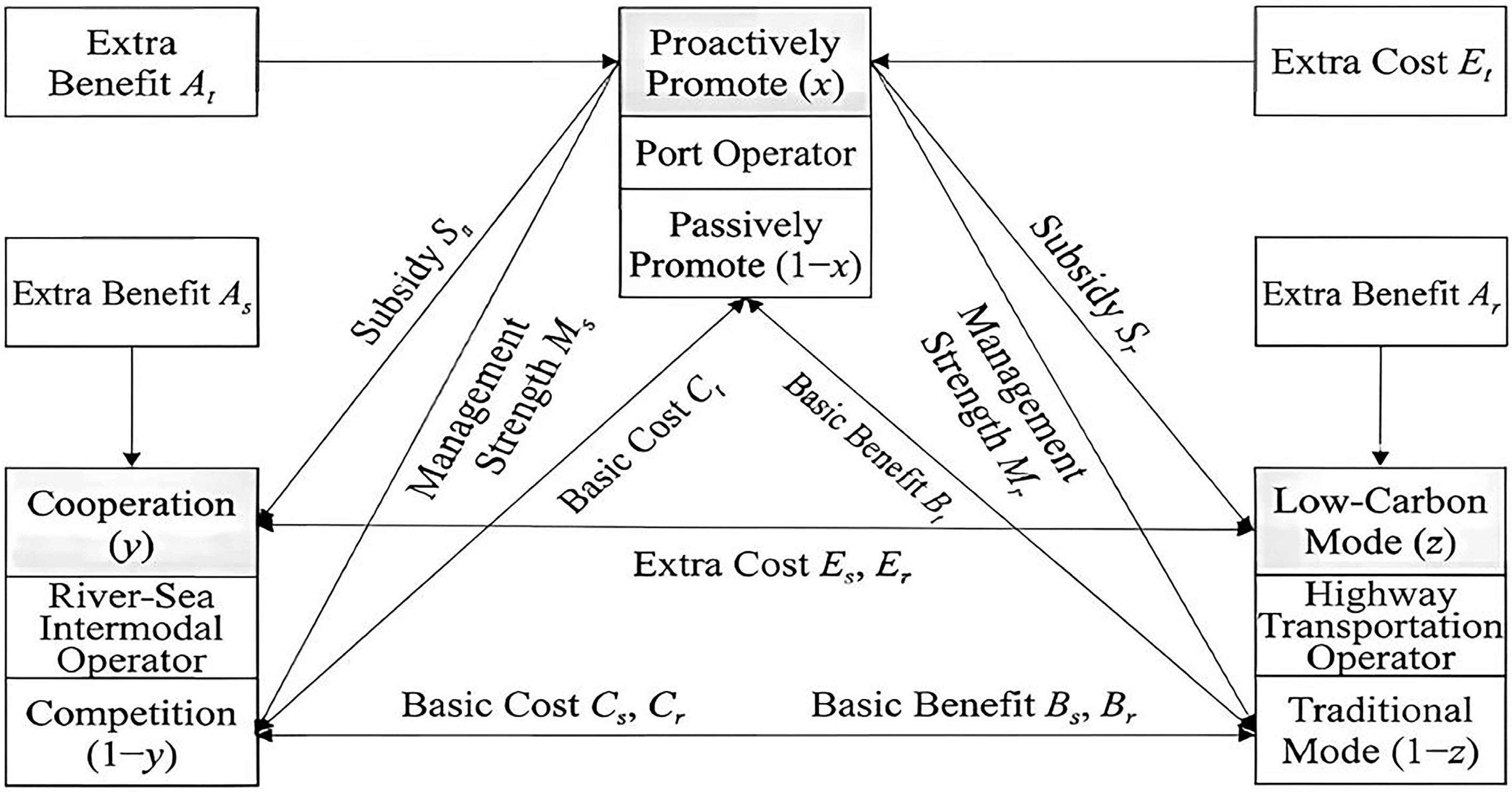
Figure 1.
Logical diagram of the tripartite evolutionary game model.
-
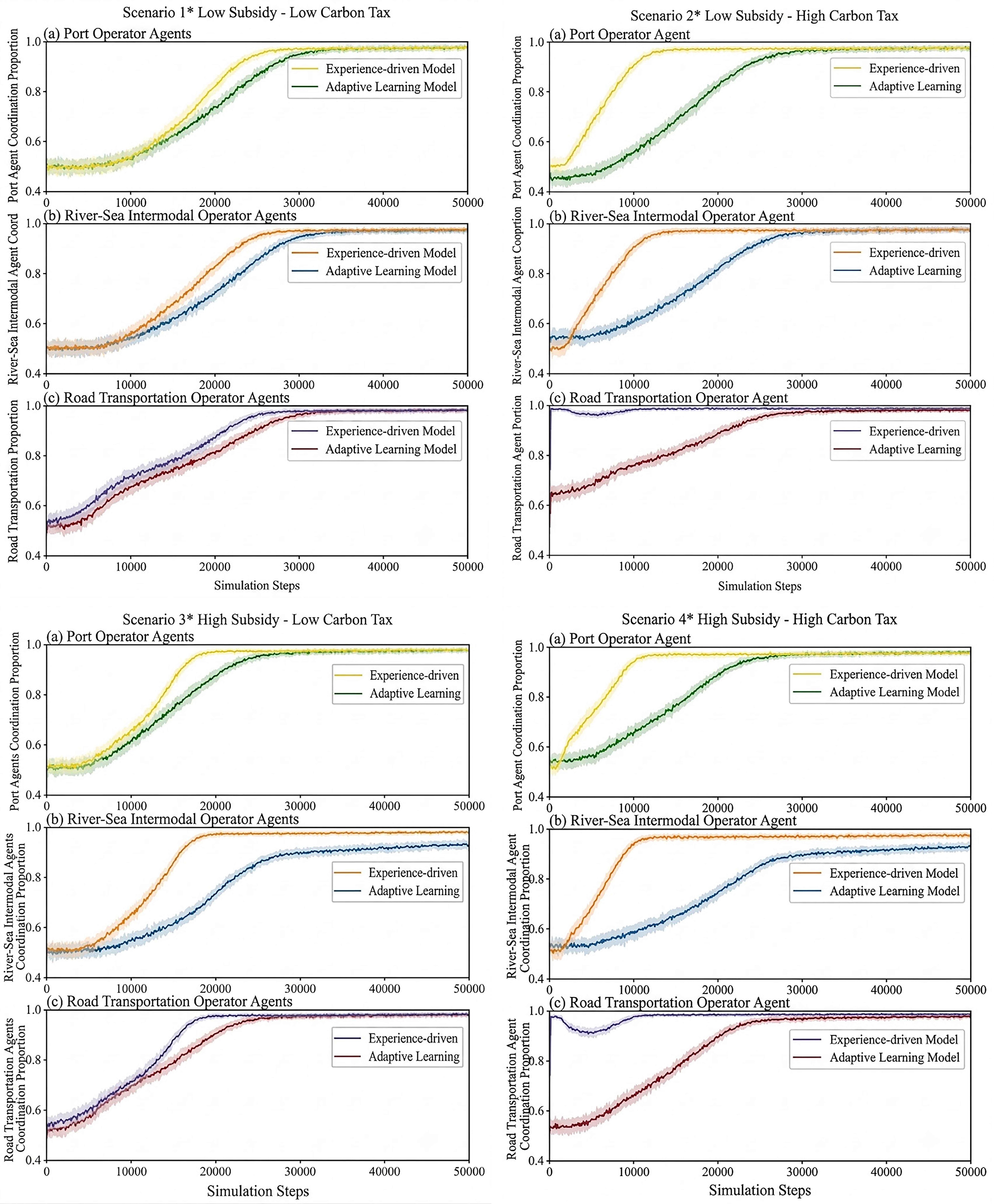
Figure 2.
System evolution trends under different policy scenarios.
-
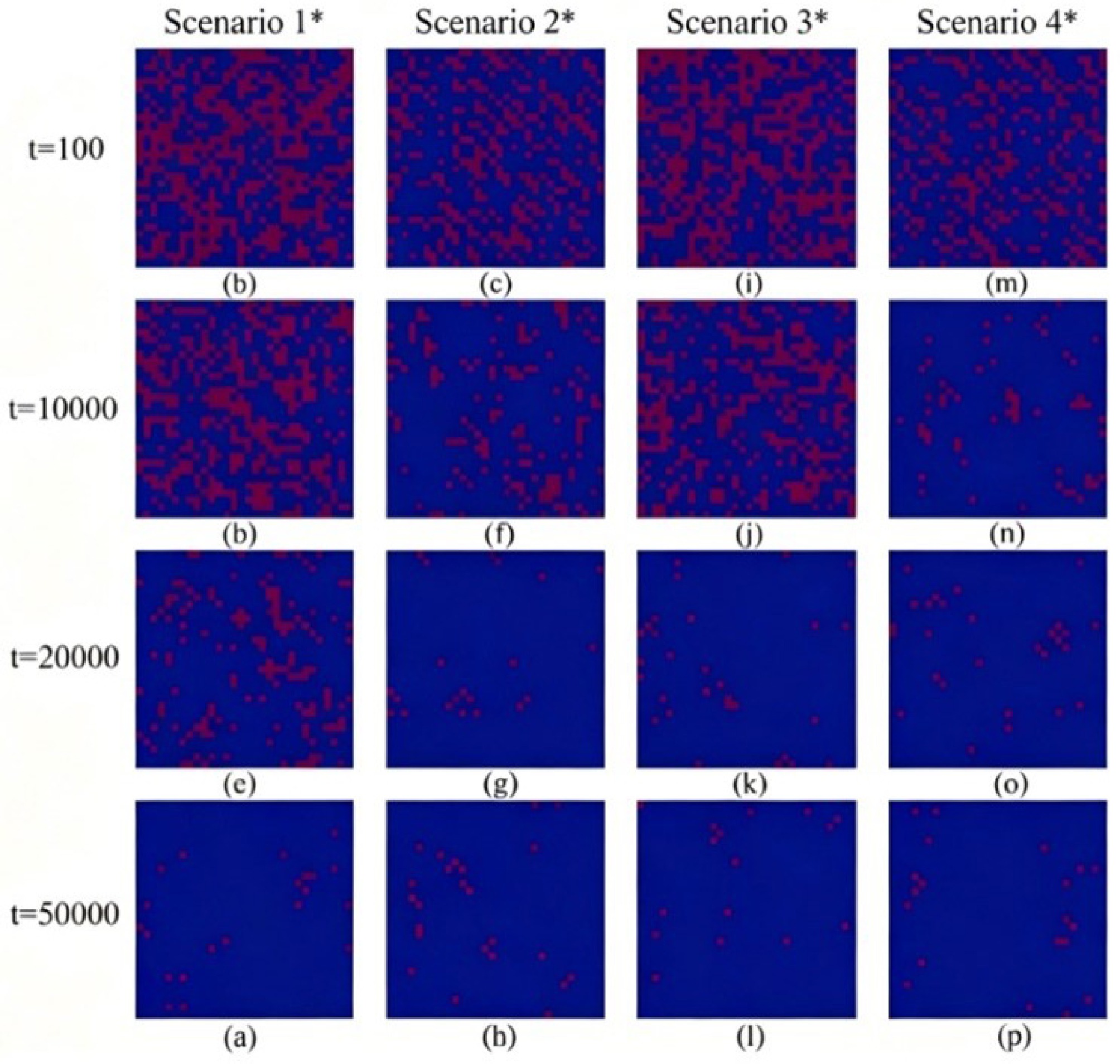
Figure 3.
Agent grid evolution under the experience-driven mode.
-
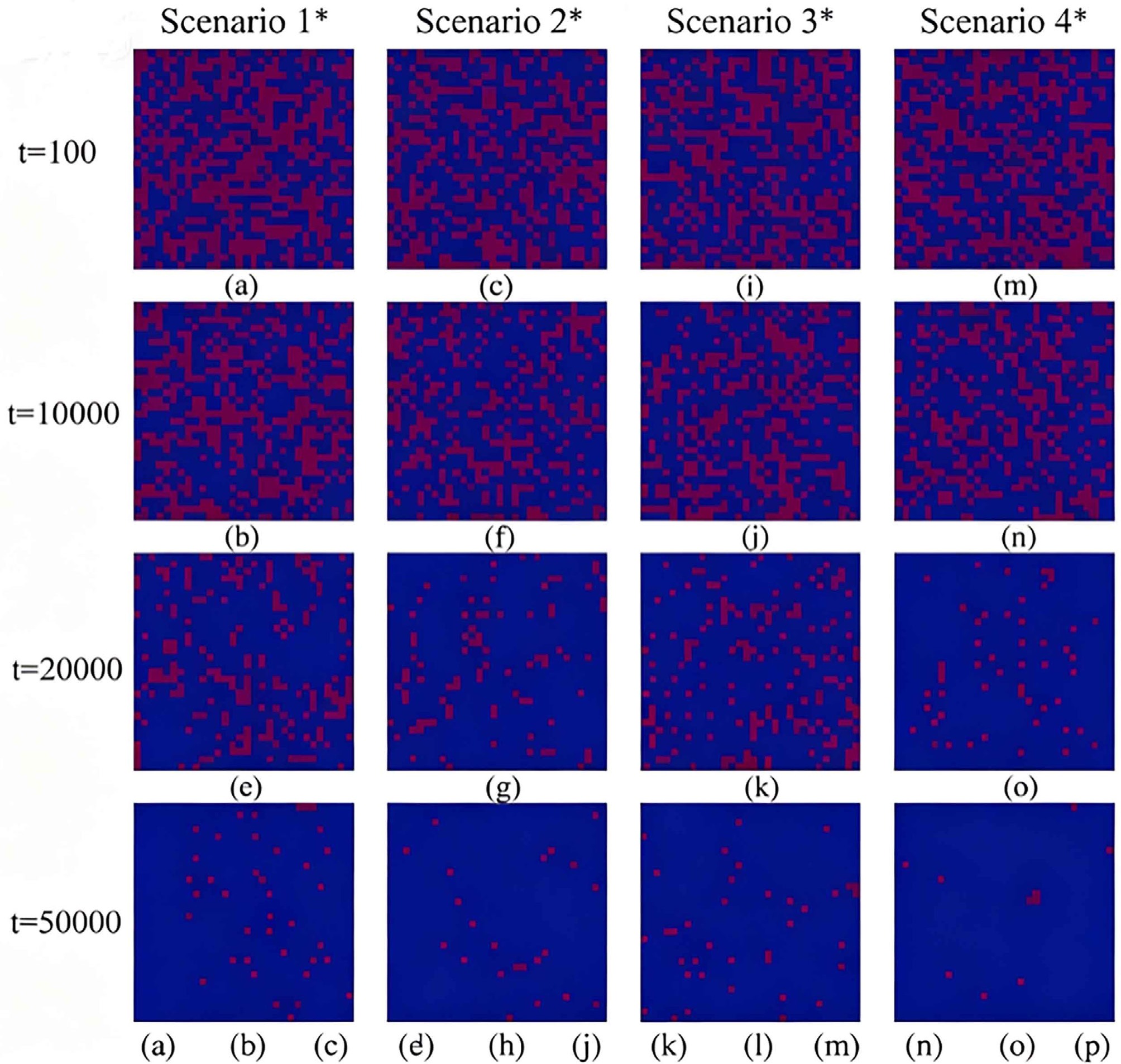
Figure 4.
Agent grid evolution under the adaptive learning mode.
-
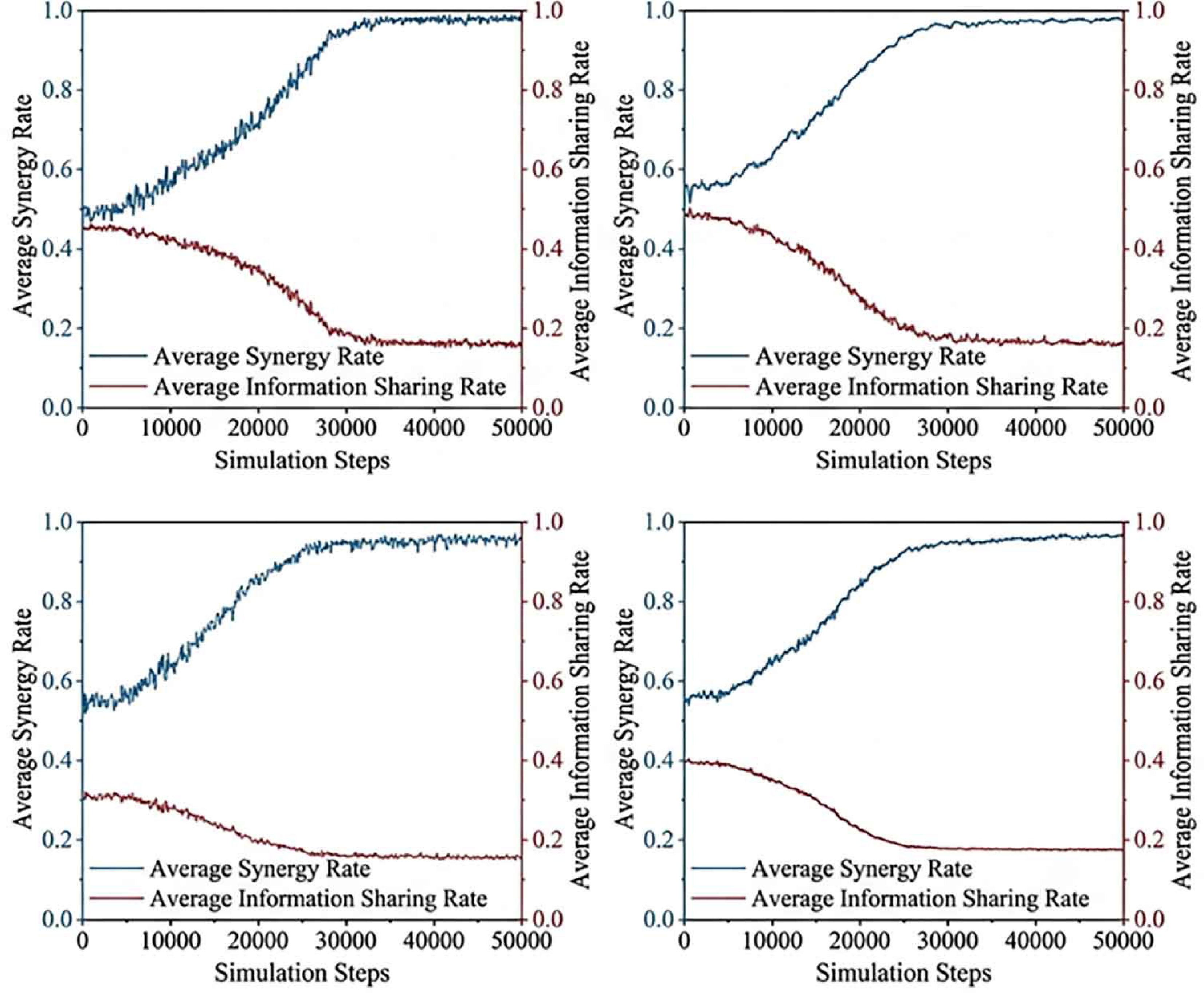
Figure 5.
Correlation trend under different scenarios.
-
Parameter Definition Description and practical significance $ {C}_{P} $ Additional costs of port green transformation Investments made by ports in green hub retrofitting and low-carbon facility
construction to enhance collaborative efficiency$ C_S $ Additional costs of river-sea intermodal transformation Additional collaborative costs incurred by intermodal operators in information
system integration and multimodal transport organization$ {C}_{R} $ Additional costs of road transport transformation Equipment renewal costs incurred during the transition of road transport
from conventional diesel-powered trucks to green energy vehicles$ {G}_{s} $ Guiding policy subsidies Phased incentives provided by the government to encourage agents to
choose green transformation, aimed at offsetting transition costs$ {T}_{c} $ Carbon tax constraint costs Punitive environmental taxes levied on the road transport sector that persists in
traditional high-emission modes, increasing evolutionary resistance$ {R}_{i} $ Baseline operating revenue Benchmark market revenue for the three types of agents ( $ i\in \left\{P,S,R\right\} $
maintaining the status quo without adopting collaborative transformation$ {R}_{c} $ Green collaborative incremental revenue Incremental profits generated by system structural optimisation and efficiency
improvement when the three agents reach a collaborative consensus$ {L}_{i} $ Collaborative failure losses Efficiency losses or congestion costs resulting from the lack of coordination
within the collection-distribution system ($ i\in \left\{P,S,R\right\} $ Table 1.
Notations and definitions for the multi-agent model.
-
Parameter category Symbol Definition Scenario 1 Scenario 2 Scenario 3 Variable parameters $ {C}_{P} $ Additional costs of port green transformation 15 20 15 $ C_S $ Additional costs of river-sea intermodal transformation 60 25 40 $ {C}_{R} $ Additional costs of road transport transformation 60 25 40 $ {T}_{c} $ Carbon tax constraint costs 15 20 15 $ {G}_{s} $ Guiding policy subsidies 4 25 40 $ {L}_{i} $ Collaborative failure losses 20 15 60 Fixed parameters $ {R}_{c} $ Green collaborative incremental revenue 55 55 55 $ {R}_{i} $ Baseline operating revenue 80 80 80 Table 2.
Simulation parameter assignments.
-
Environmental state $ s_{i}^{t} $ Port (C, T) River–Sea intermodal (C, T) Road transport (C, T) (0,0) 135 85 138 31 124 56 (0,1) 107 181 119 249 146 68 (0,2) 304 126 244 257 76 168 (1,0) 116 153 35 129 147 91 (1,1) 302 164 270 152 326 131 (1,2) 307 276 274 215 327 135 (2,0) 17 260 0 161 45 259 (2,1) 275 288 276 188 329 275 (2,2) 308 288 276 259 332 300 The bold values are the steady Q-values. Table 3.
Steady-state Q-values under the low subsidy, low carbon tax scenario.
-
Environmental state $ s_{i}^{t} $ Port (C, T) River–sea intermodal (C, T) Road transport (C, T) (0,0) 111 13 123 67 126 8 (0,1) 64 219 168 122 51 182 (0,2) 102 240 103 218 61 206 (1,0) 232 121 82 143 307 107 (1,1) 311 220 151 239 333 153 (1,2) 334 269 303 219 334 186 (2,0) 215 121 177 8 259 178 (2,1) 334 228 119 290 332 217 (2,2) 337 321 306 296 341 308 The bold values are the steady Q-values. Table 4.
Steady-state Q-values under the low subsidy, high carbon tax scenario.
-
Environmental state $ s_{i}^{t} $ Port (C, T) River–sea intermodal (C, T) Road transport (C, T) (0,0) 4 0 3 0 266 58 (0,1) 0 213 310 27 135 188 (0,2) 59 552 335 131 71 320 (1,0) 332 275 0 74 466 160 (1,1) 606 119 73 308 605 214 (1,2) 608 556 336 307 620 451 (2,0) 0 352 79 0 615 211 (2,1) 384 557 334 256 621 492 (2,2) 621 563 336 317 621 537 The bold values are the steady Q-values. Table 5.
Steady-state Q-values under the high subsidy, low carbon tax scenario.
-
Environmental state $ s_{i}^{t} $ Port (C, T) River–sea intermodal (C, T) Road transport (C, T) (0,0) 369 96 53 336 0 203 (0,1) 71 390 361 206 0 322 (0,2) 568 0 0 270 60 421 (1,0) 279 387 354 156 148 358 (1,1) 596 349 369 281 317 568 (1,2) 532 565 375 303 621 418 (2,0) 584 328 190 328 374 574 (2,1) 613 557 370 345 626 576 (2,2) 618 575 377 371 633 588 The bold values are the steady Q-values. Table 6.
Steady-state Q-values under the high subsidy, high carbon tax scenario.
Figures
(5)
Tables
(6)