-
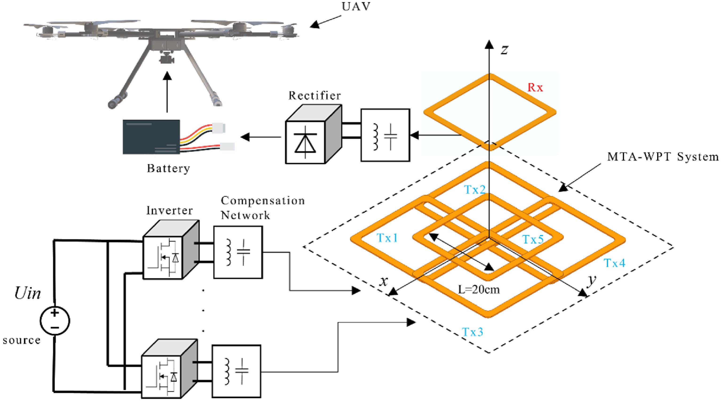
Figure 1.
Schematic diagram of the MTA-WPT system.
-
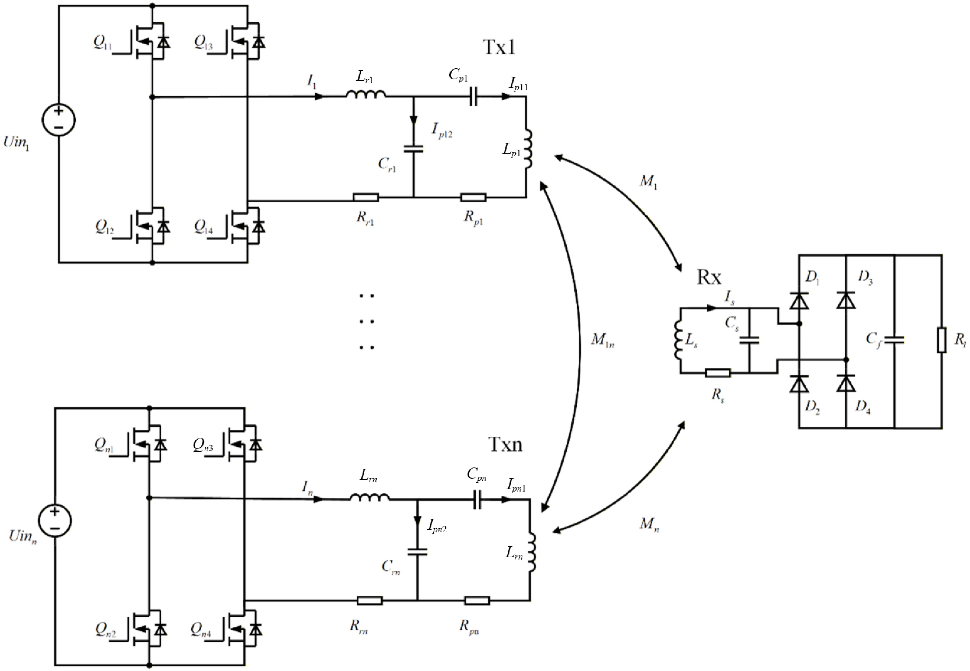
Figure 2.
MTA-WPT system circuit model.
-
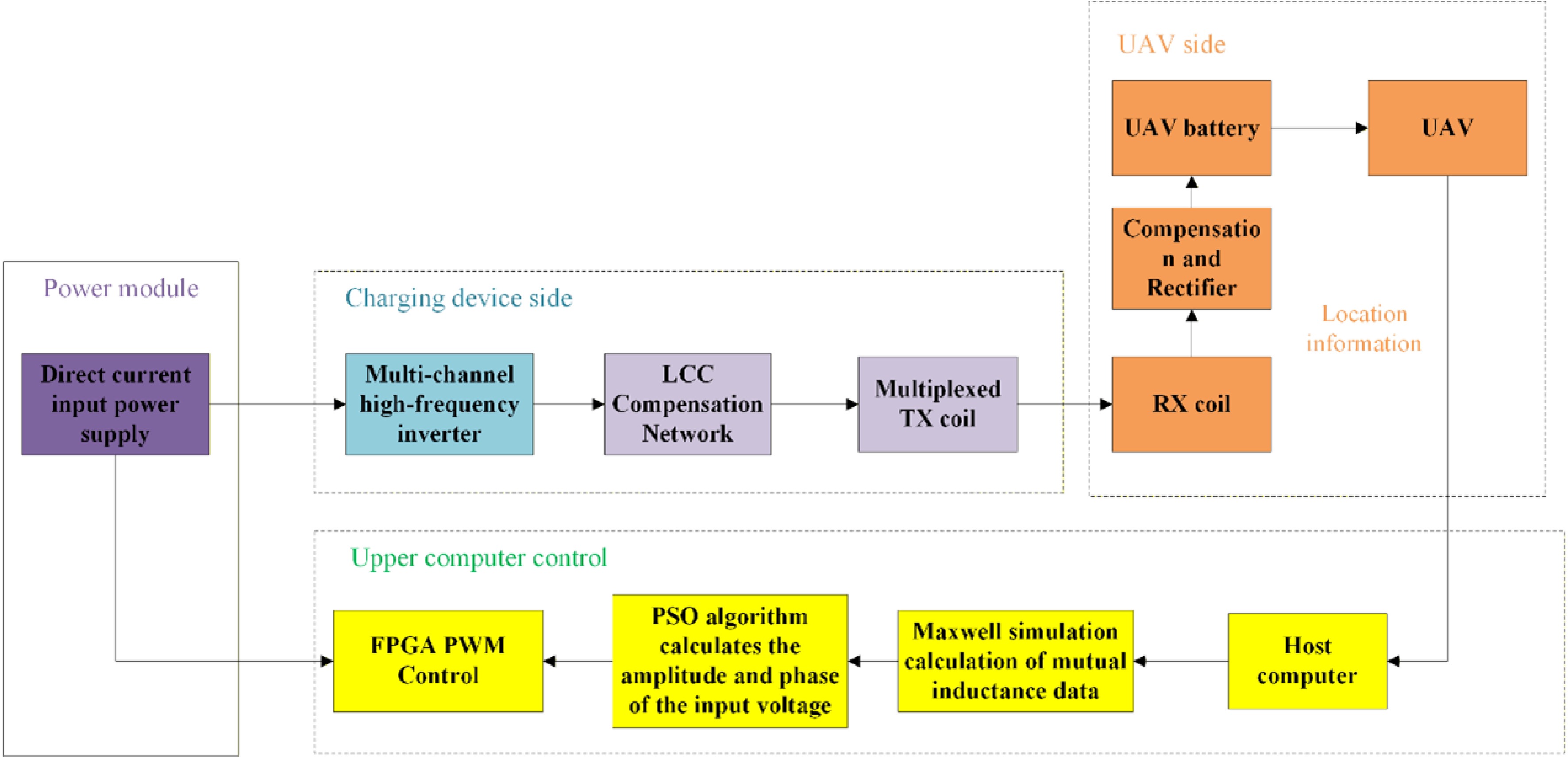
Figure 3.
Structure diagram of unmanned aerial vehicle charging system.
-
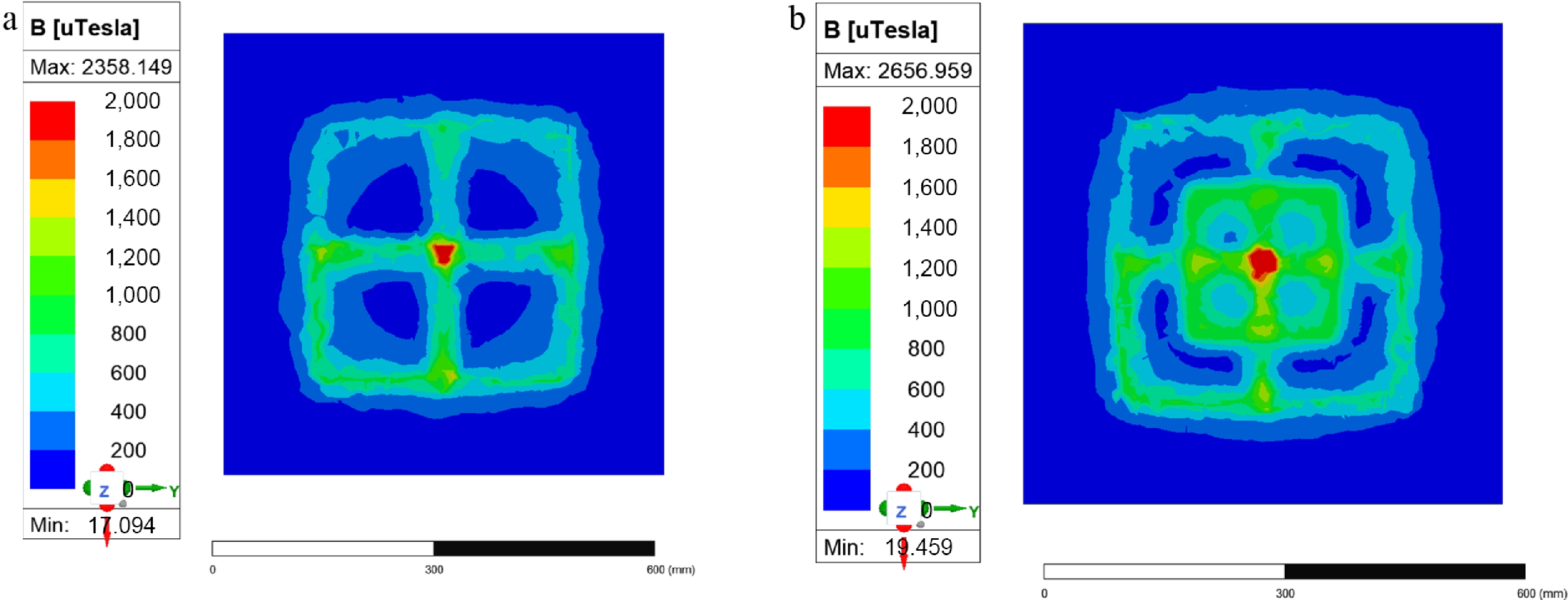
Figure 4.
(a) Simulation diagram of four-coil magnetic field strength. (b) Simulation diagram of five-coil magnetic field strength.
-
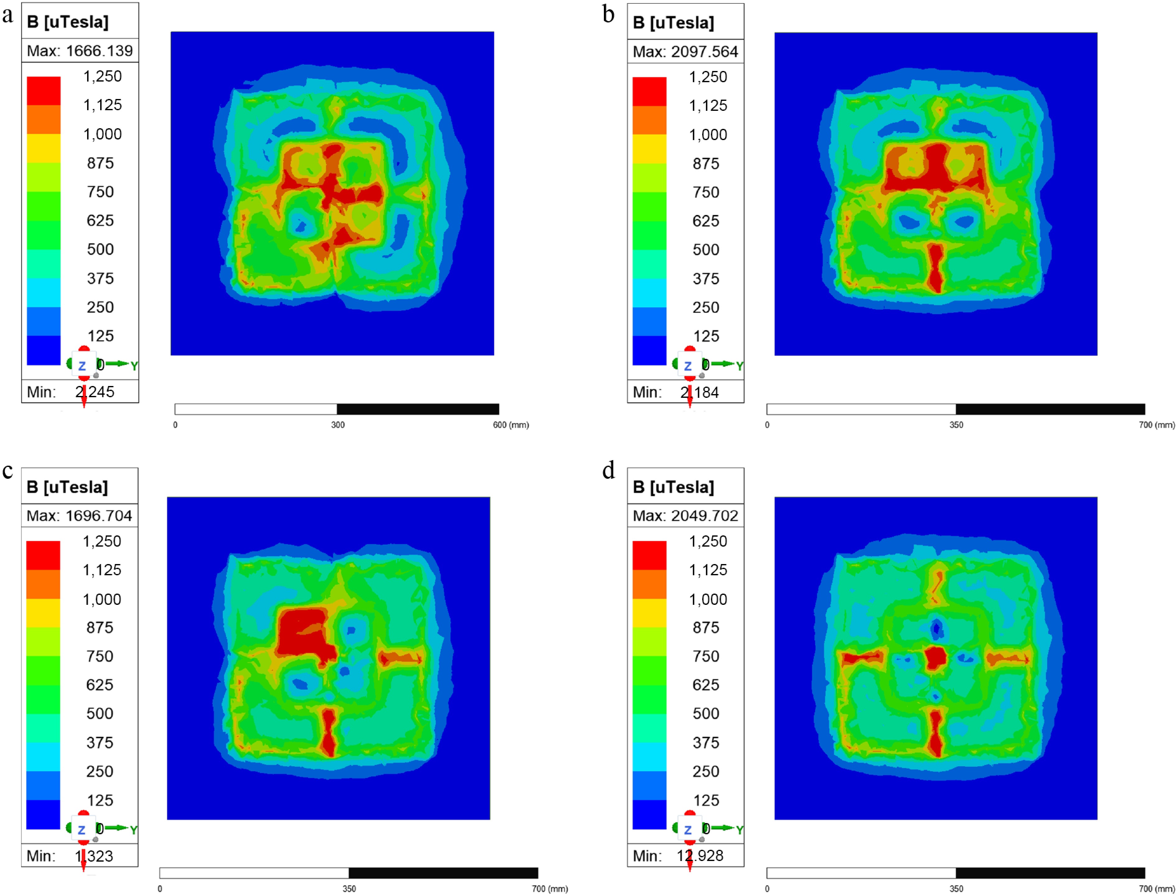
Figure 5.
(a) Tx1 is offset by 180°. (b) Tx1 and Tx2 are offset by 180°. (c) Tx1, Tx2, and Tx3 are offset by 180°. (d) Tx1, Tx2, Tx3, and Tx4 are offset by 180°.
-
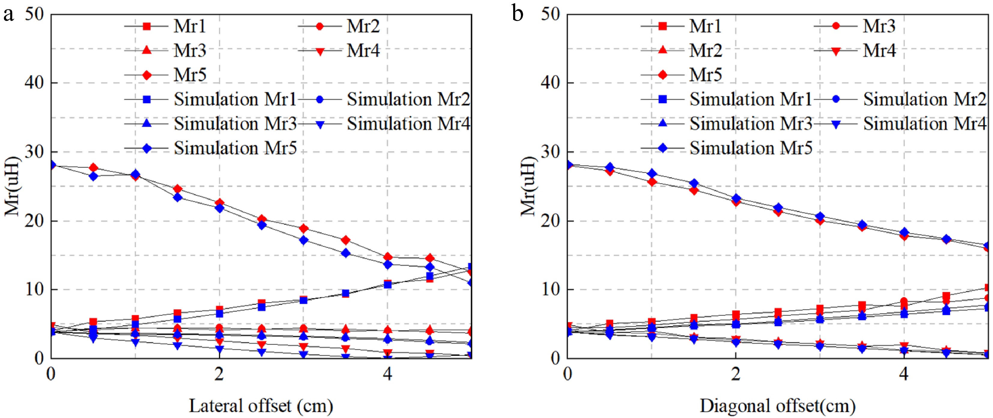
Figure 6.
The mutual inductance experiment and simulation results between the receiving coil and the five-antenna coil: (a) Lateral offset mutual inductance diagram, (b) diagonal offset mutual inductance diagram.
-
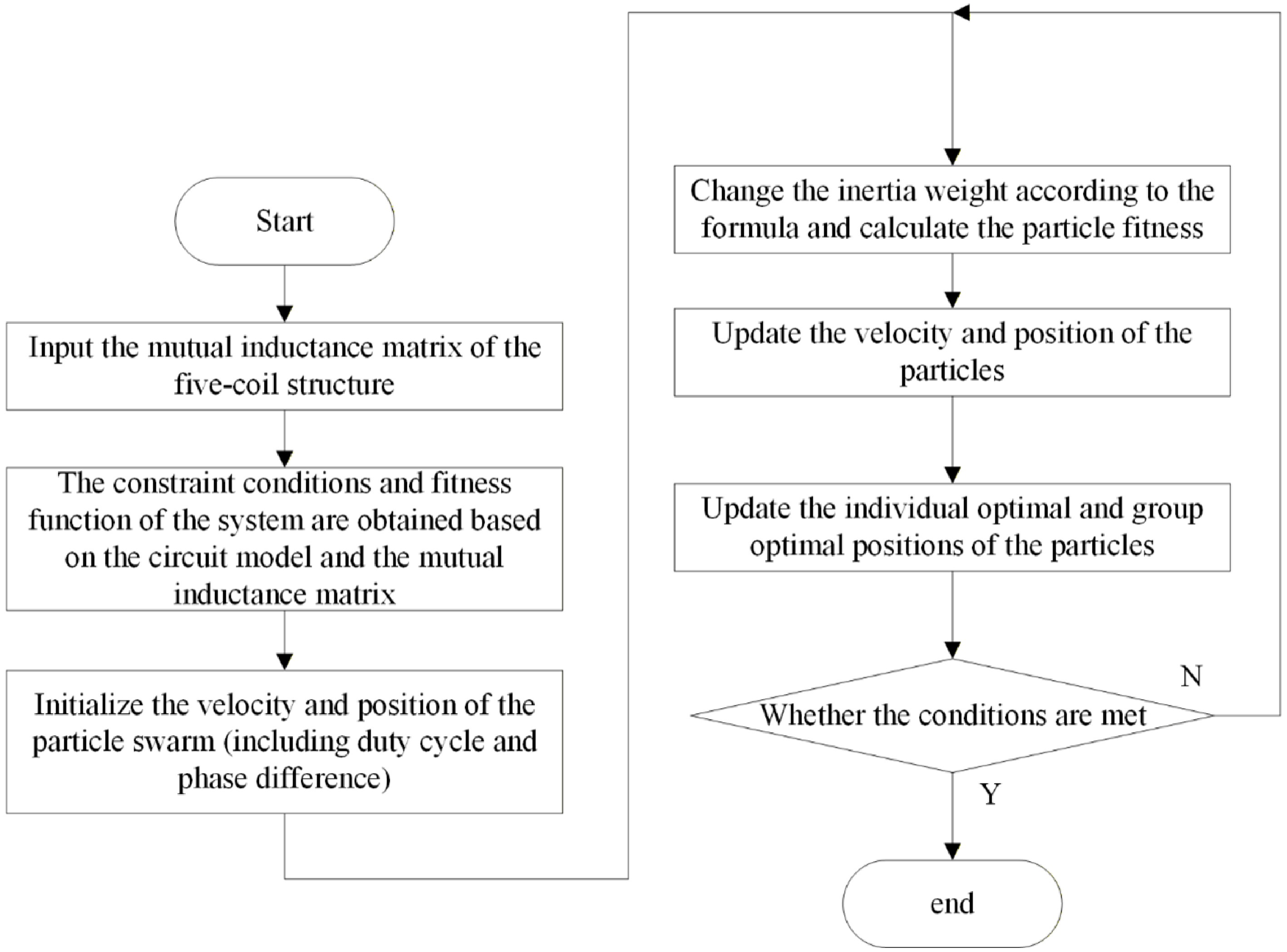
Figure 7.
Specific implementation steps of the particle swarm algorithm.
-
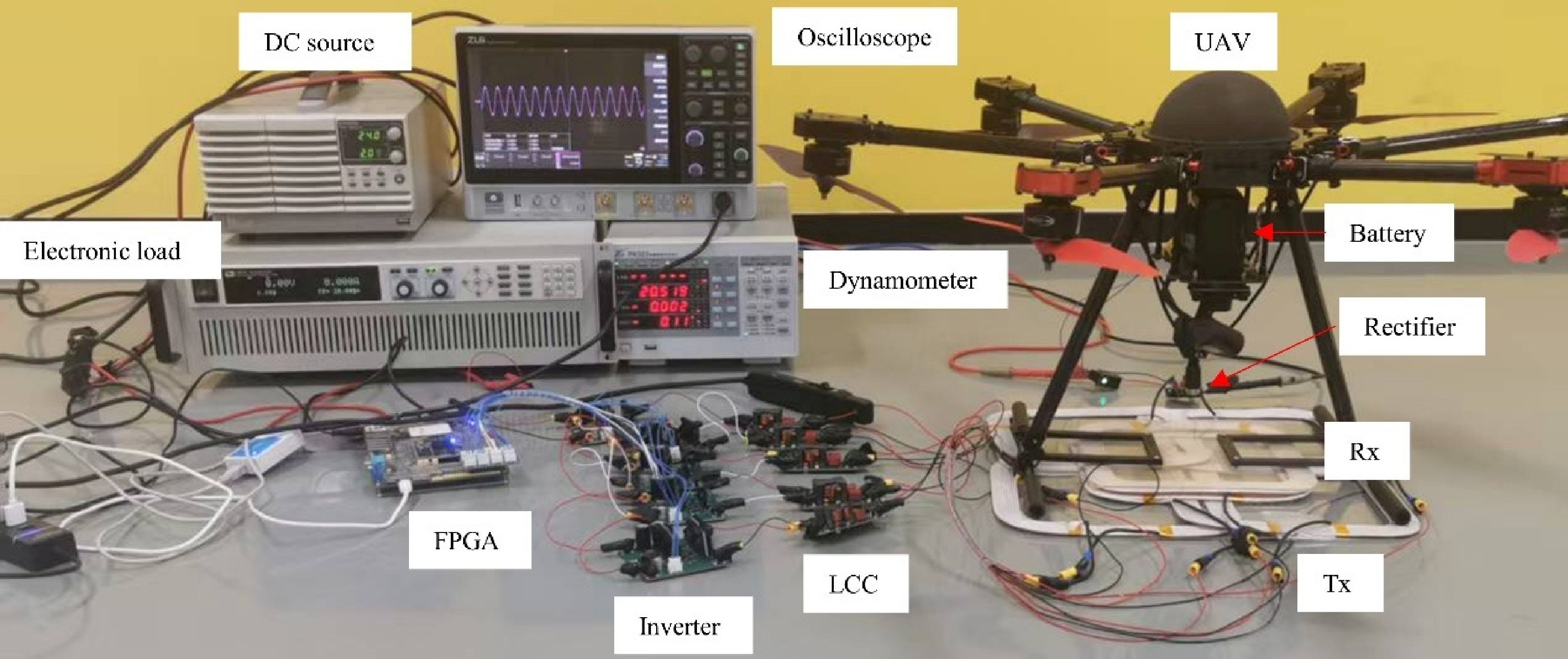
Figure 8.
MTA-WPT system experimental prototype.
-
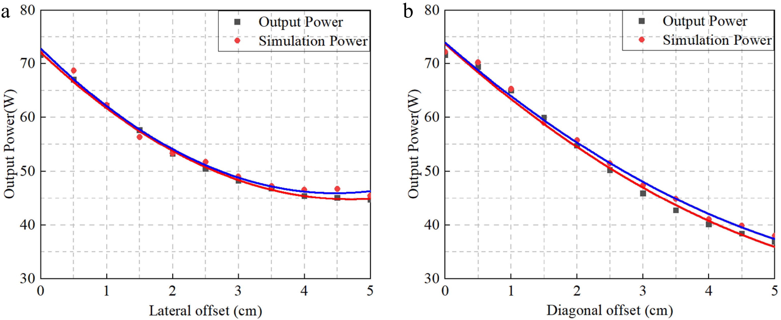
Figure 9.
Comparison of simulated and measured output power: (a) lateral offset; (b) diagonal offset.
-
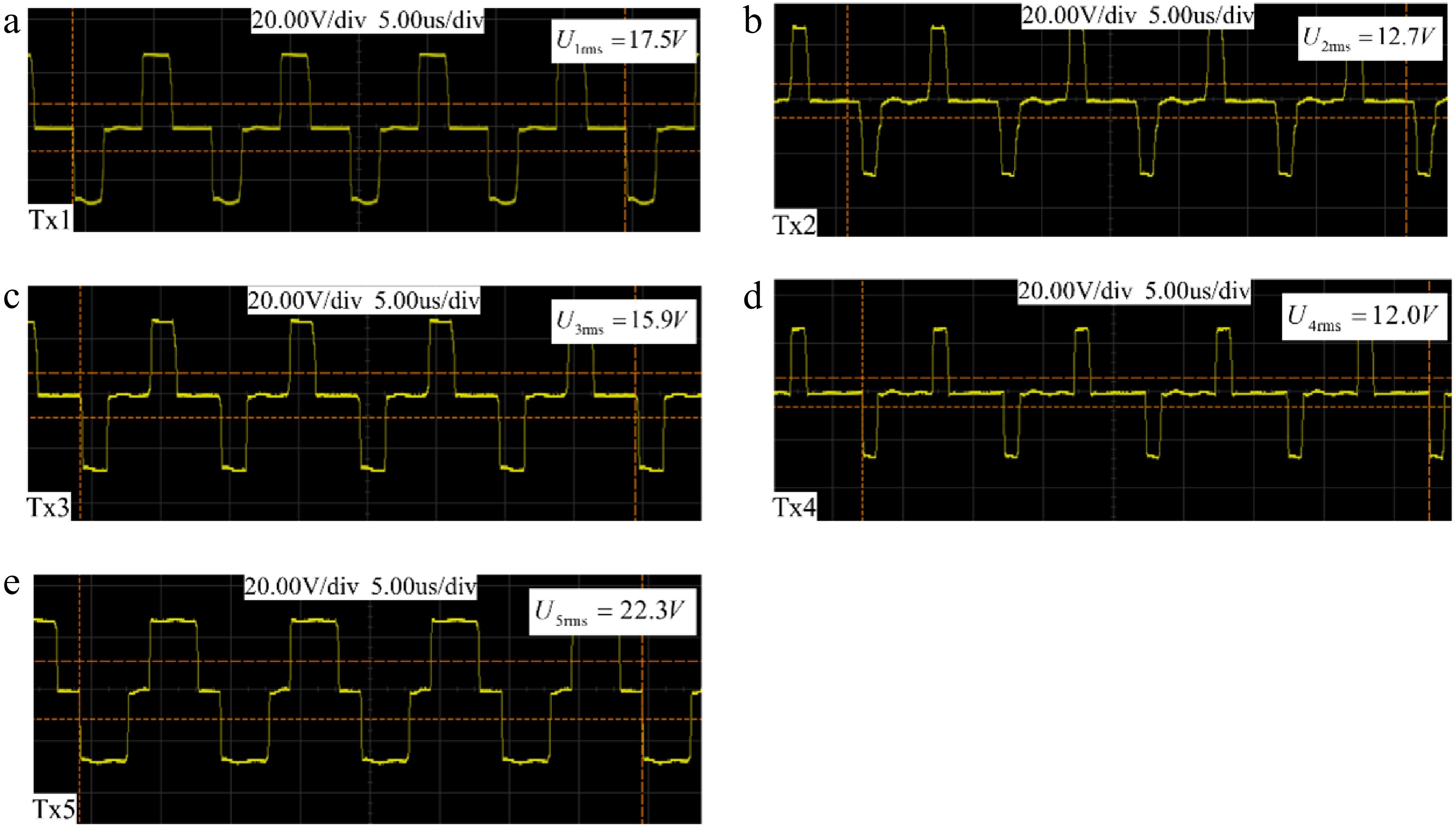
Figure 10.
Output voltages of the five-channel inverters. (a) Tx1. (b) Tx2. (c) Tx3. (d) Tx4. (e) Tx5.
-
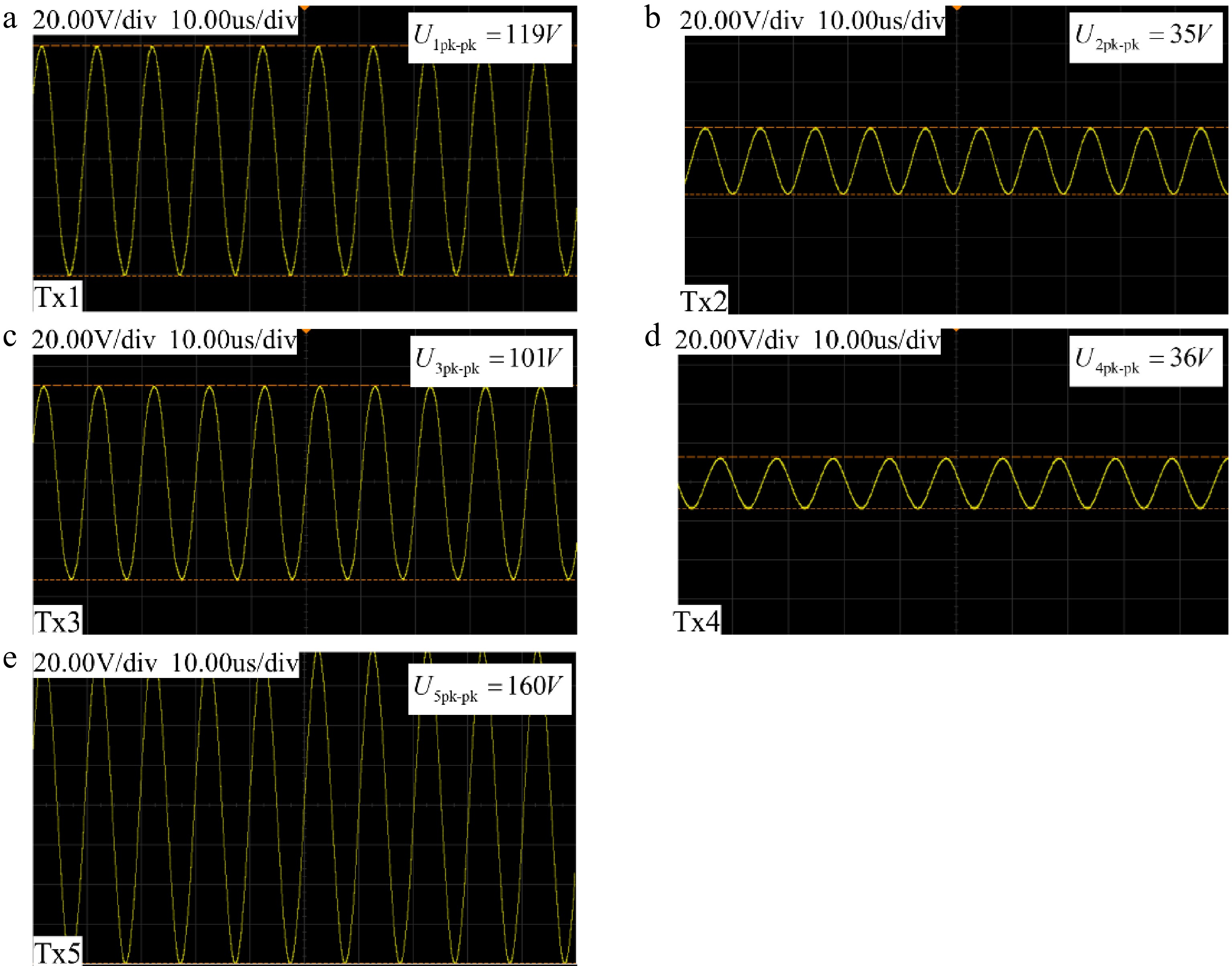
Figure 11.
Input voltage of the five-channel Tx coil. (a) Tx1. (b) Tx2. (c) Tx3. (d) Tx4. (e) Tx5.
-
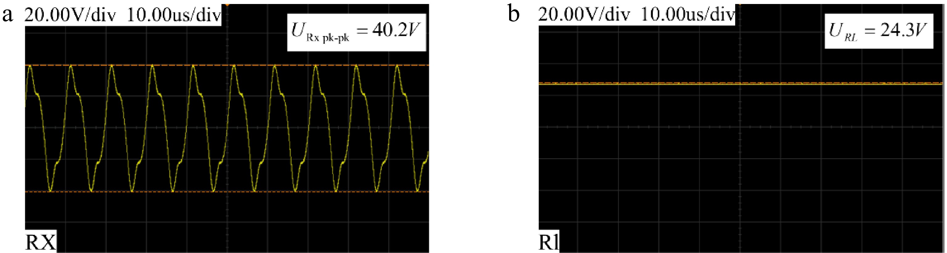
Figure 12.
(a) Output voltage of the Rx coil; (b) Input voltage of the load.
-
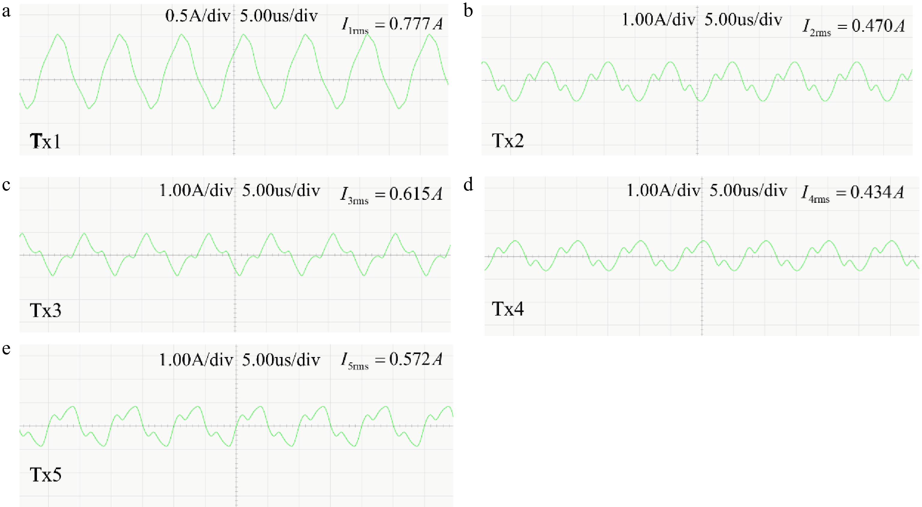
Figure 13.
Output currents of the five-channel inverters. (a) Tx1. (b) Tx2. (c) Tx3. (d) Tx4. (e) Tx5.
-
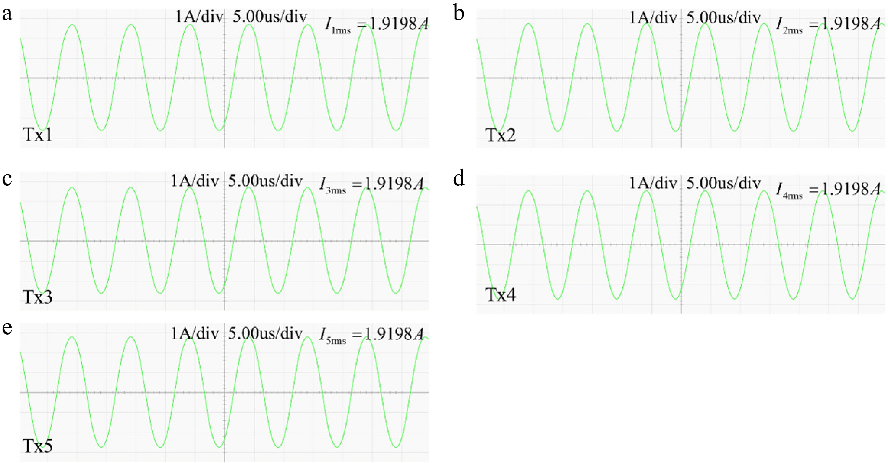
Figure 14.
Input currents of the five-channel Tx coil. (a) Tx1. (b) Tx2. (c) Tx3. (d) Tx4. (e) Tx5.
-
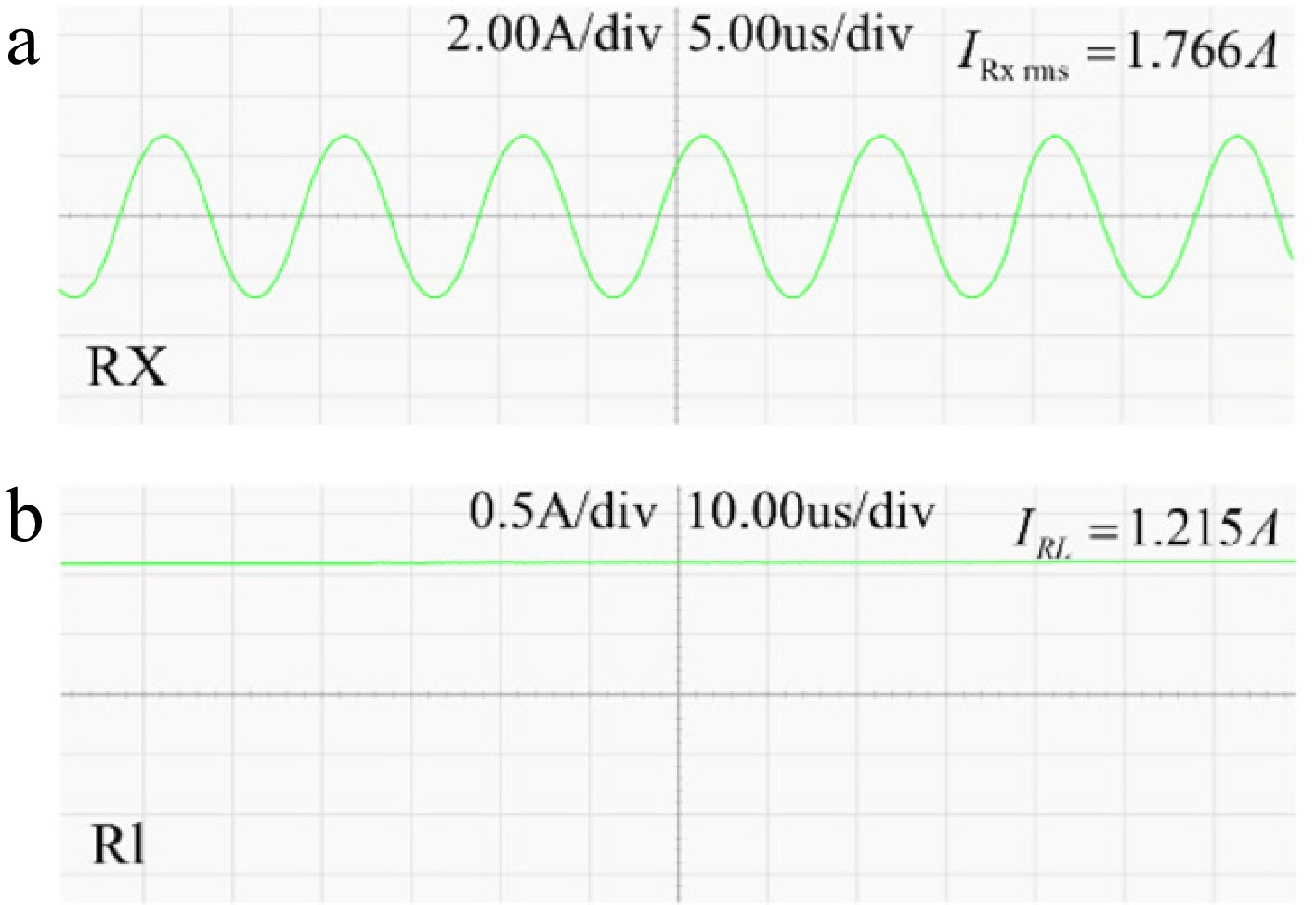
Figure 15.
(a) Output current of the Rx coil; (b) Input current of the load.
-
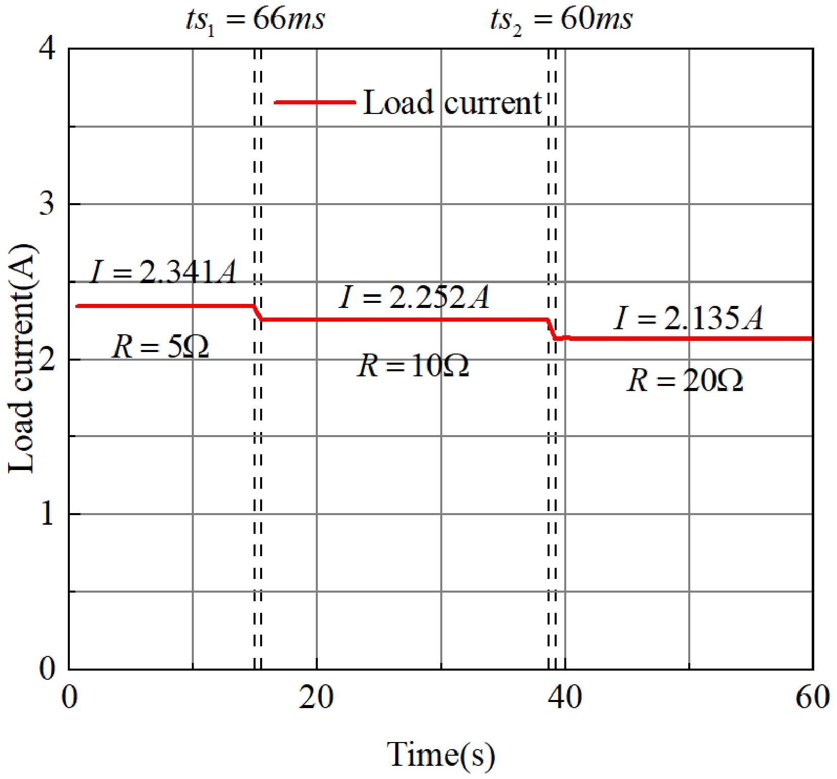
Figure 16.
The load current varies with the load.
-
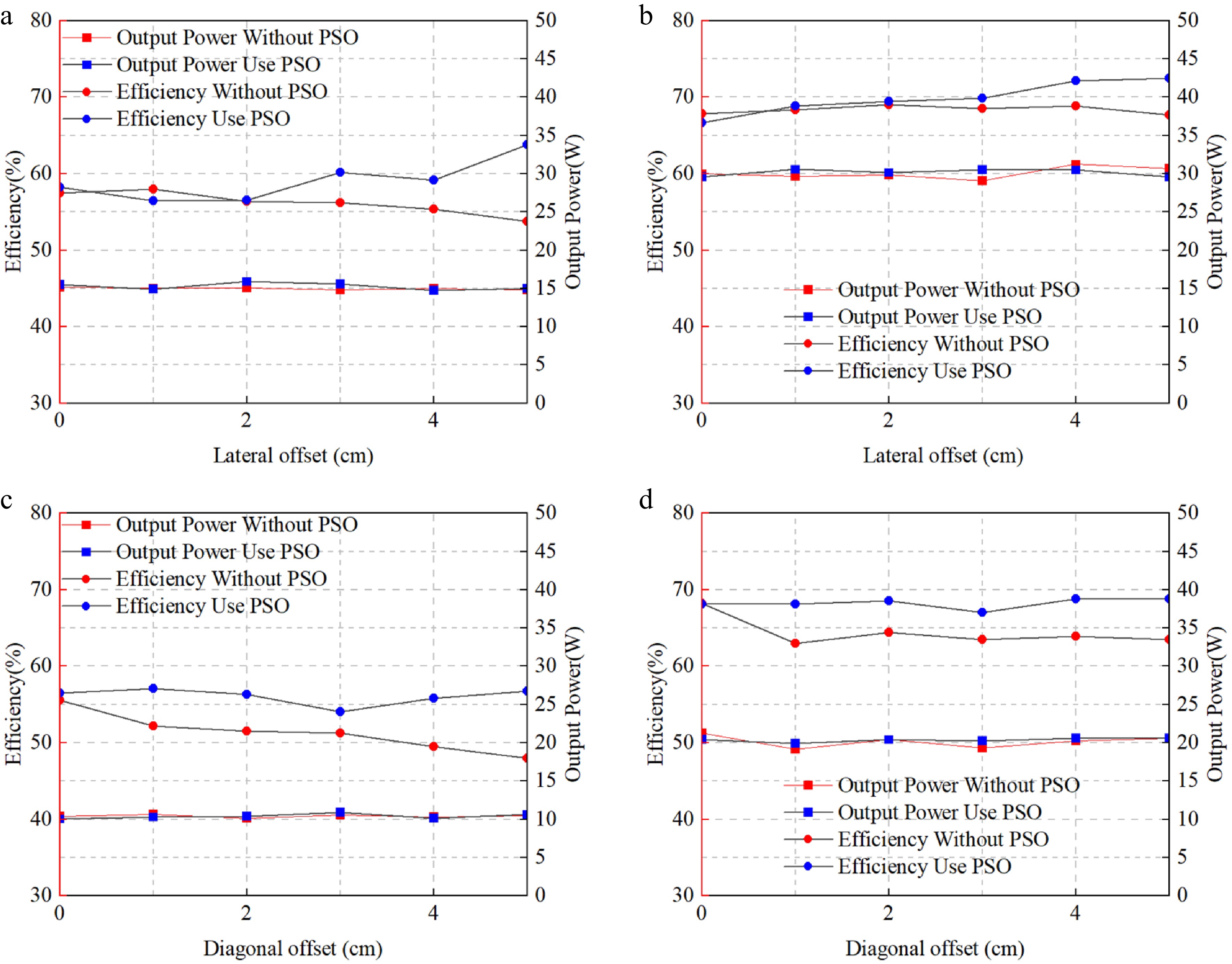
Figure 17.
(a) Efficiency curve at 15 W with 10
$ \Omega $ $ \Omega $ $ \Omega $ $ \Omega $ -
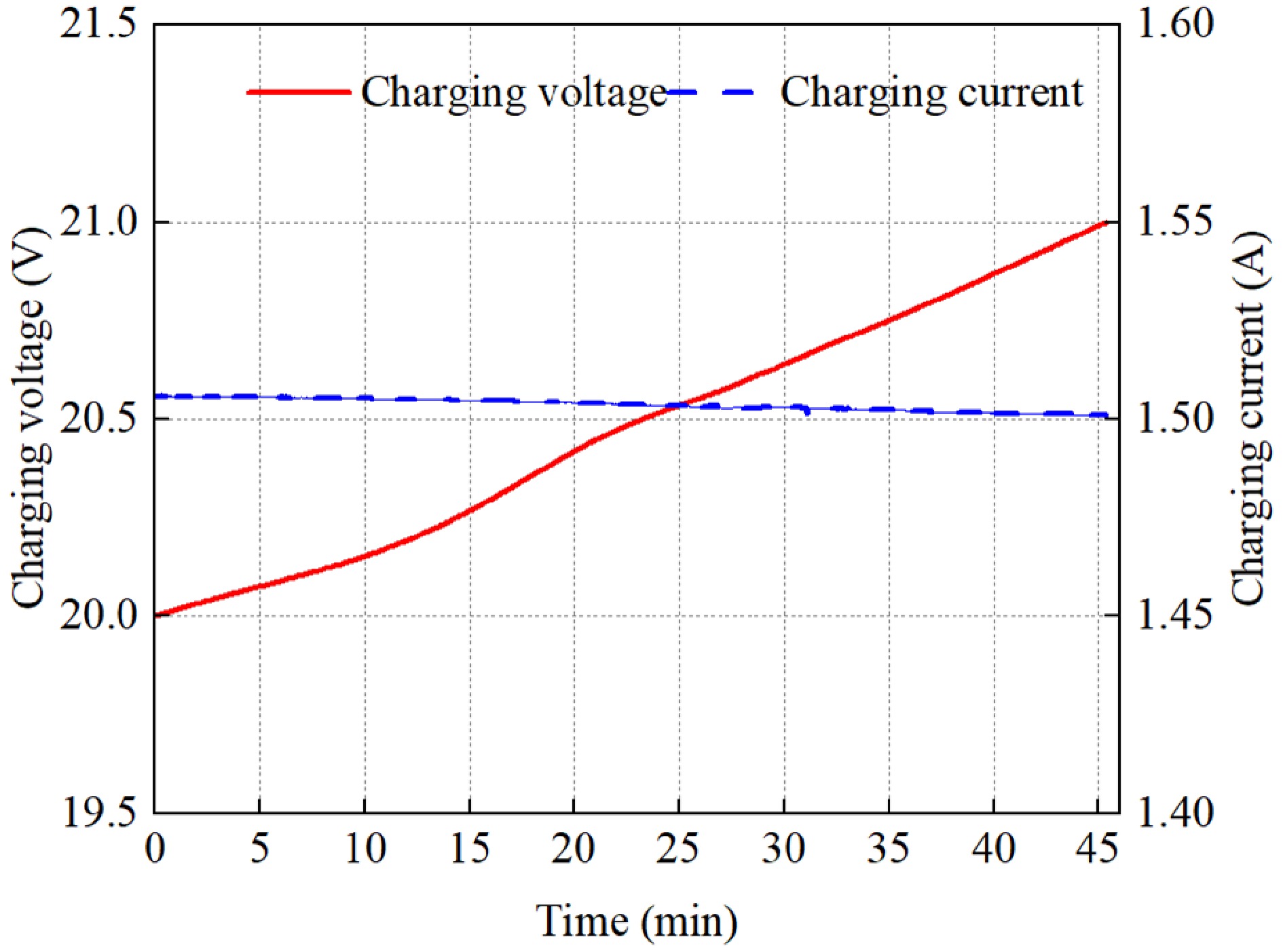
Figure 18.
The charging voltage and current under a 5 cm diagonal offset.
-
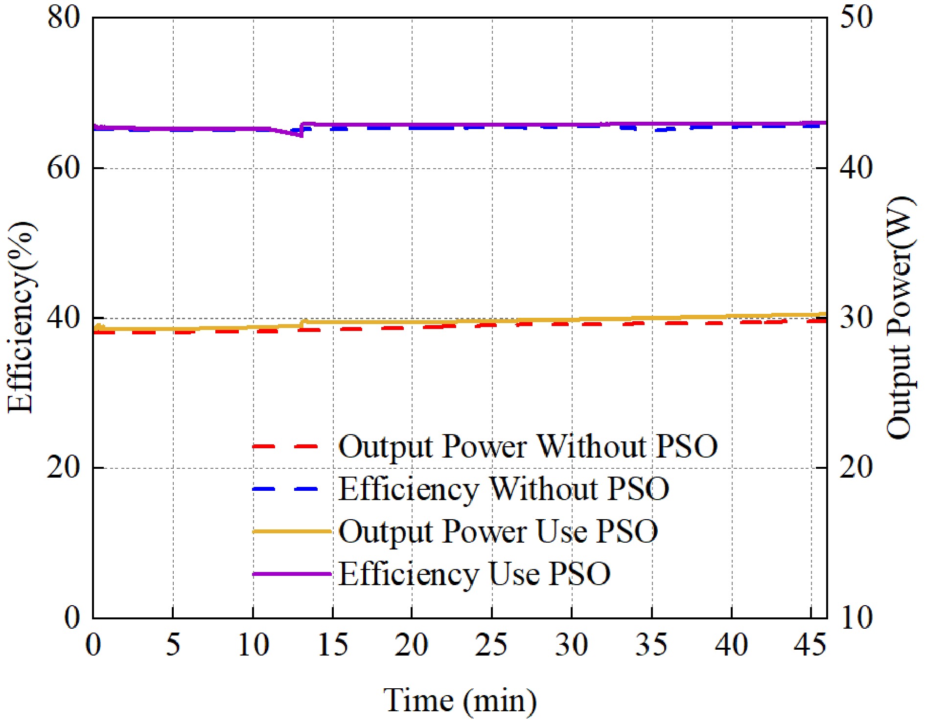
Figure 19.
Charging power and efficiency diagram of the receiving coil at the center of the coil array.
-
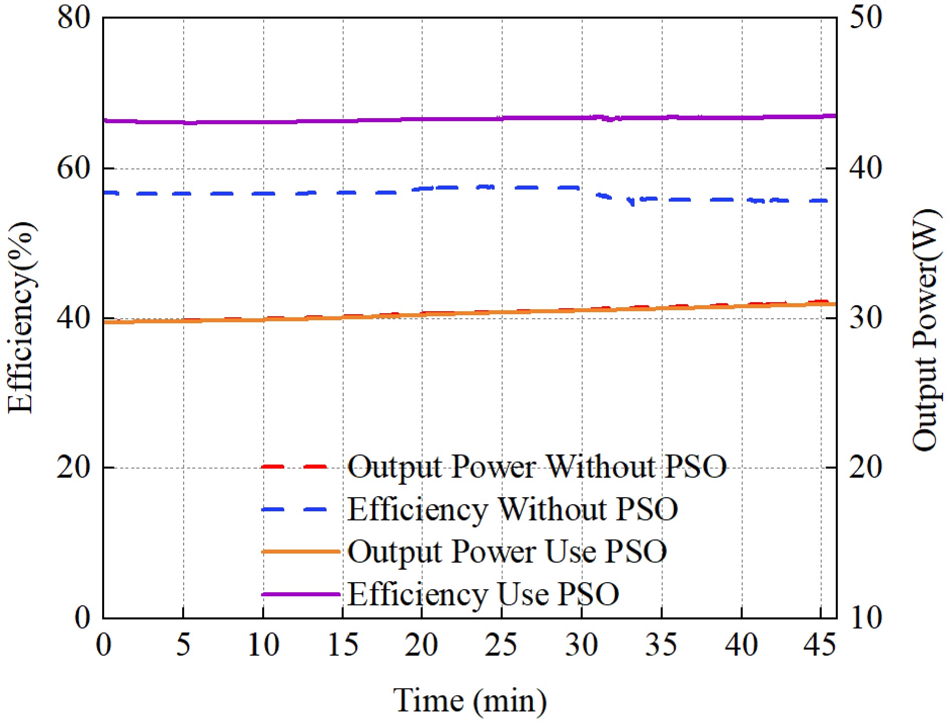
Figure 20.
Charging power and efficiency graph with the transverse offset of the receiving coil by 5 cm.
-
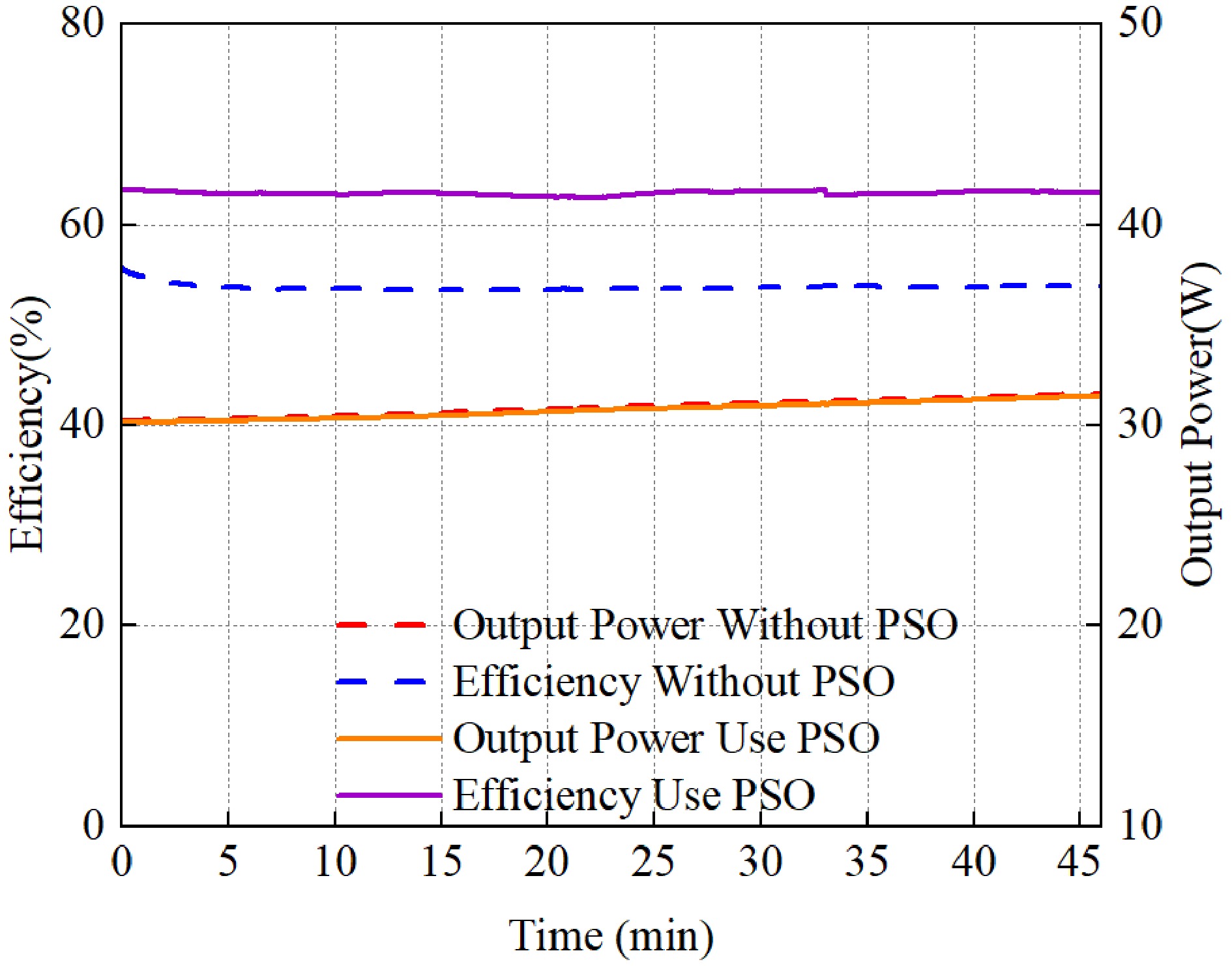
Figure 21.
Graph showing the charging power and efficiency when the diagonal offset of the receiving coil is 5 cm.
-
Parameter Experiment value Parameter Experiment value $ Uin $ 24 V $ {L}_{s} $ 37 μH $ f $ 100 kHz $ {C}_{s} $ 64.7 nF $ {L}_{r} $ 15 μH $ {R}_{r} $ 145 m $ \Omega $ $ {C}_{r} $ 163 nF $ {R}_{p} $ 236 m $ \Omega $ $ {C}_{p} $ 110 nF $ {R}_{s} $ 236 m $ \Omega $ $ {L}_{p} $ 37 μH $ {R}_{l} $ 130 $ \Omega $ Table 1.
MTA-WPT system parameters.
-
Self-inductance and mutual inductance $ {L}_{1} $ $ {M}_{12} $ $ {M}_{13} $ $ {M}_{14} $ $ {M}_{15} $ $ {M}_{1} $ $ {M}_{21} $ $ {L}_{2} $ $ {M}_{23} $ $ {M}_{24} $ $ {M}_{25} $ $ {M}_{2} $ $ {M}_{31} $ $ {M}_{32} $ $ {L}_{3} $ $ {M}_{34} $ $ {M}_{35} $ $ {M}_{3} $ $ {M}_{41} $ $ {M}_{42} $ $ {M}_{43} $ $ {L}_{4} $ $ {M}_{45} $ $ {M}_{4} $ $ {M}_{51} $ $ {M}_{52} $ $ {M}_{53} $ $ {M}_{54} $ $ {L}_{5} $ $ {M}_{5} $ $ {M}_{1} $ $ {M}_{2} $ $ {M}_{3} $ $ {M}_{4} $ $ {M}_{5} $ $ {L}_{6} $ Self-inductance and mutual inductance values 37.0863 0.621815 0.461625 1.866375 4.252525 10.3442 0.621815 39.8564 2.363775 0.5875 4.2872 0.747275 0.461625 2.363775 37.1706 0.439625 4.222975 8.8188 1.866375 0.5875 0.439625 37.4132 4.6258 0.83975 4.252525 4.2872 4.222975 4.6258 38.4432 16.01258 10.3442 0.747275 8.8188 0.83975 16.01258 36.6945 Table 2.
The mutual inductance M matrix under the condition of a 5 cm lateral offset.
-
Parameter Parameter value Position variables (including four phase differences and duty ratios) –90°~90°; 0.05~0.5 Number of particles $ N $ 50 Number of iterations iter 100 Speed variable $ v $ −5~5; −0.02~0.02 Inertia weight $ w $ 0.4~0.9 Learning factor $ {c}_{1} $ $ {c}_{2} $ 1.5 Proportional coefficient $ {h}_{1} $ $ {h}_{2} $ 0.75, 0.25 Penalty coefficient $ penalt{y}_{1} $ $ penalt{y}_{2} $ 0.05, 0.1 Table 3.
Algorithm parameter settings.
-
Offset distance (cm) Efficiency without PSO
for 10$ \Omega $ Efficiency use PSO for 10 $ \Omega $ Efficiency without PSO for 20 $ \Omega $ Efficiency use PSO for 20 $ \Omega $ 0 57.4933 58.23086 67.85213 66.66081 1 57.989 56.47121 68.33018 68.84291 2 56.35397 56.53843 69.02037 69.42831 3 56.19405 60.18519 68.50459 69.87048 4 55.33274 59.14359 68.86572 72.12933 5 53.75083 63.80204 67.68607 72.51287 Output power (W) 15 15 30 30 Table 4.
Efficiency comparison under horizontal offset.
-
Offset distance (cm) Efficiency without PSO for 10 $ \Omega $ Efficiency use PSO for 10 $ \Omega $ Efficiency without PSO for 20 $ \Omega $ Efficiency use PSO for 20 $ \Omega $ 0 55.59878 56.5317 68.22239 68.14133 1 52.20701 57.12194 62.98619 68.1694 2 51.52683 56.29865 64.40019 68.58894 3 51.25058 54.06424 63.50154 67.0334 4 49.53487 55.81579 63.8911 68.78317 5 48.01168 56.78205 63.4688 68.78317 Output power (W) 10 10 20 20 Table 5.
Efficiency comparison under diagonal offset.
Figures
(21)
Tables
(5)