










-
Wireless power transfer (WPT), as a contactless power delivery method, offers advantages such as convenience, safety, reliability, and environmental adaptability[1,2]. It reduces risks associated with physical connectors, such as wear, sparking, and explosion, thereby providing essential technological support for the continuous autonomous operation of devices. WPT shows broad application prospects in various fields, including electric vehicles[3−5], power supply and monitoring for underwater equipment[6−8], and wireless charging for unmanned systems such as UAV[9,10].
Among these applications, autonomous charging for unmanned aerial vehicles (UAVs) is a particularly valuable research direction. In long-duration missions, endurance is a key bottleneck for UAV performance. However, during autonomous landing, factors such as navigation inaccuracy and environmental disturbances (e.g., wind) often cause deviation between the actual landing position and the preset charging platform center. This misalignment significantly affects the relative positioning and coupling between transmitter and receiver coils, thereby degrading the system's power transfer efficiency[11].
To enhance the misalignment tolerance of WPT systems, several approaches have been studied, including different coupler structures[12,13], improving landing accuracy[14], implementing primary-side and secondary-side control[15,16], adopting different compensation topologies[17], and applying impedance matching techniques[18]. While these methods partially improve tolerance to misalignment, they still struggle to meet the charging requirements of UAVs over large, arbitrary landing areas. In recent years, multi-transmitter coil array systems have attracted increasing research attention. Such structures can significantly expand the effective charging area and improve anti-misalignment performance[19,20].
To address the instability in power and efficiency caused by positional offset in multi-transmitter array systems, various methods have been proposed, focusing on coil array geometry, suppression of cross-coupling, and control of system inputs. In terms of coil array structures, these can be categorized into 2-D planar arrays[21] and 3-D orthogonal arrays[22]. In 3-D orthogonal structures, output control is typically achieved by regulating the amplitude and phase of currents. However, 2-D planar arrays offer greater scalability. In planar parallel coil arrangements, magnetic field cancellation may occur in certain regions. To mitigate this, improvements have been made to both primary and secondary coil designs: primary coils can be stacked[23], while secondary coils may adopt asymmetric structures that encompass multiple primary coils[24].
In multi-coil systems, cross-coupling among transmitting coils increases reactive power and reduces overall system efficiency. For two-coil systems, cross-coupling can be minimized by overlapping the coils[25]. For systems with more than two coils, variable reactance methods may be employed to suppress cross-coupling[26].
System power and efficiency can be controlled from either the primary or secondary side. However, to extend UAV flight time, minimizing weight on the secondary side is preferred. Therefore, in this work, system performance is regulated by controlling the input—specifically the amplitude, phase, and frequency of the excitation. For a two-transmitter (Tx) coil system with adjustable current amplitude, the optimal current ratio between the two Tx coils is equal to the ratio of their coupling coefficients with the receiver[27]. By analyzing the phase effect on power via magnetic flux angle measurements and using a BP neural network to learn the phase–current relationship of the magnetic flux, the influence of phase on power has been validated[28]. Simultaneous amplitude and phase control in multi-coil arrays can enhance the system's transmission efficiency coefficient[29]. By predefining the frequency and phase of Tx coil currents and employing suitable dual-frequency quad-phase combinations, multi-Tx WPT systems can provide full positional and rotational charging freedom to the receiving (Rx) coil[30].
Thus, output power control is essential in WPT systems. While operating frequency is usually fixed, controlling the amplitude and phase of the input voltage is relatively straightforward. To compensate for efficiency losses due to receiver displacement, this paper proposes a multiple-transmitter-array WPT system. By regulating the amplitude and phase of the input voltage, the system achieves constant-power charging with high efficiency even when the UAV is offset from the intended landing position.
The paper is organized as follows. The Materials and methods section models and analyzes the MTA-WPT system, focusing on the circuit model of a five-coil system. The Multi-input coil amplitude and phase optimization algorithm section presents an optimization algorithm for the amplitude and phase of the multiple input coils using a particle swarm optimization (PSO) approach. The Results section provides experimental and simulation analyses of the optimal efficiency search algorithm for the MTA-WPT system, including prototype construction and testing, constant-current charging experiments, and efficiency comparisons under lateral and diagonal offsets. Finally, the Conclusions section summarizes the main findings.
-
To achieve constant current charging for the UAV during the charging process, the system adopts an LCC-P compensation topology, which exhibits near-constant-current characteristics on the load side. Figure 1 shows the schematic diagram of the MTA-WPT system. The designed MTA-WPT system employs five transmitting coils and one receiving coil. All transmitting coils are powered by a single source and share identical configurations, but each has a dedicated inverter and compensation circuit. Input voltage amplitude and phase control for the multi-transmitter system is realized by modulating the PWM waveform fed to each inverter.
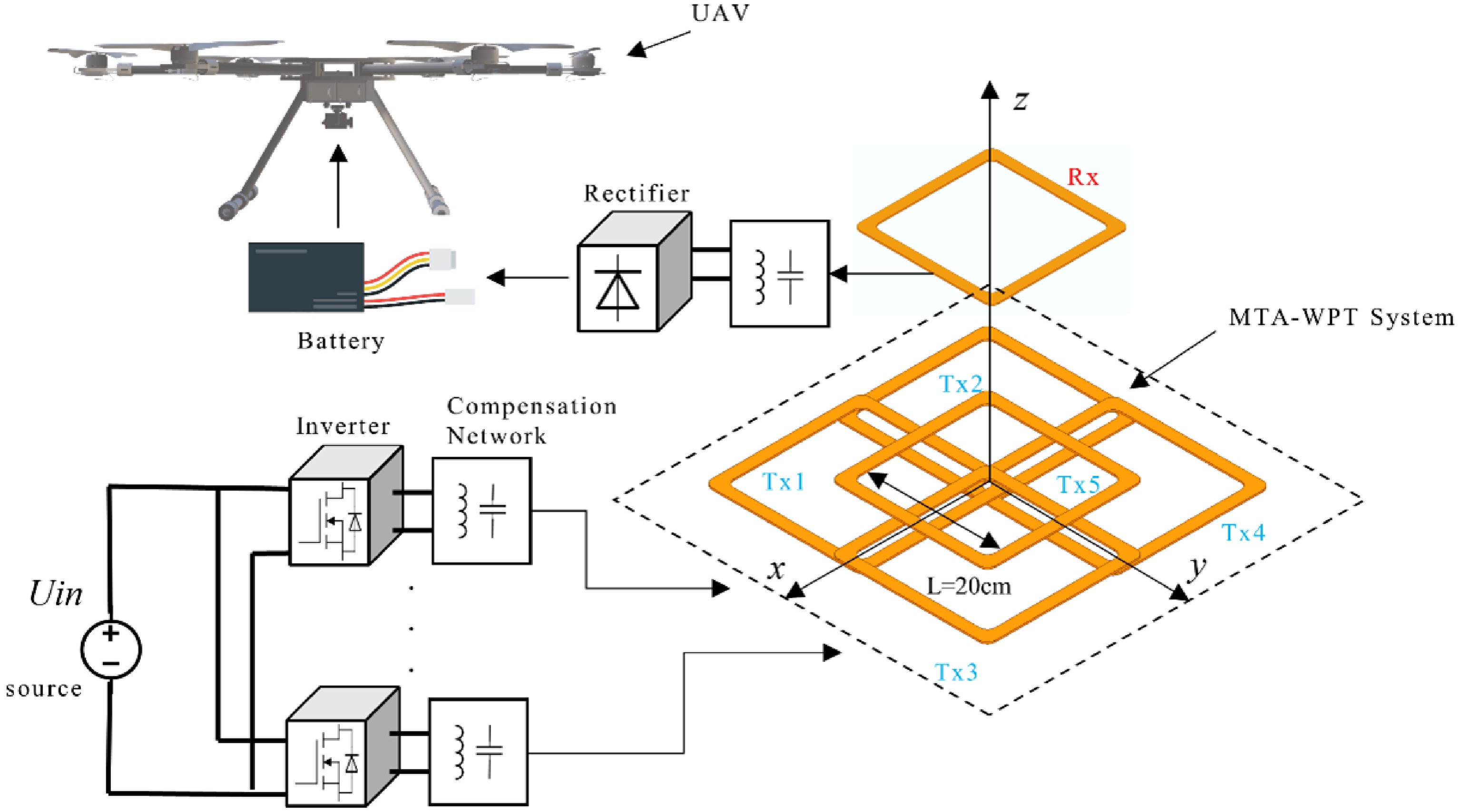
Figure 1.
Schematic diagram of the MTA-WPT system.
Figure 2 illustrates the circuit model of the system. Figure 3 Structure diagram of the unmanned aerial vehicle charging system.
$ {L}_{rn} $ $ {C}_{rn} $ $ {C}_{pn} $ $ {L}_{pn} $ $ {L}_{s} $ $ {C}_{s} $ $ {R}_{rn} $ $ {R}_{pn} $ $ {R}_{s} $ $ {M}_{ij} $ $ 1\leq i, j\leq n $ $ {M}_{i} $ $ 1\leq i\leq n $ $ i $ $ {R}_{l} $ $ {R}_{L}=\dfrac{8}{{\text{π} }^{2}}{R}_{l} $ $ \omega $ 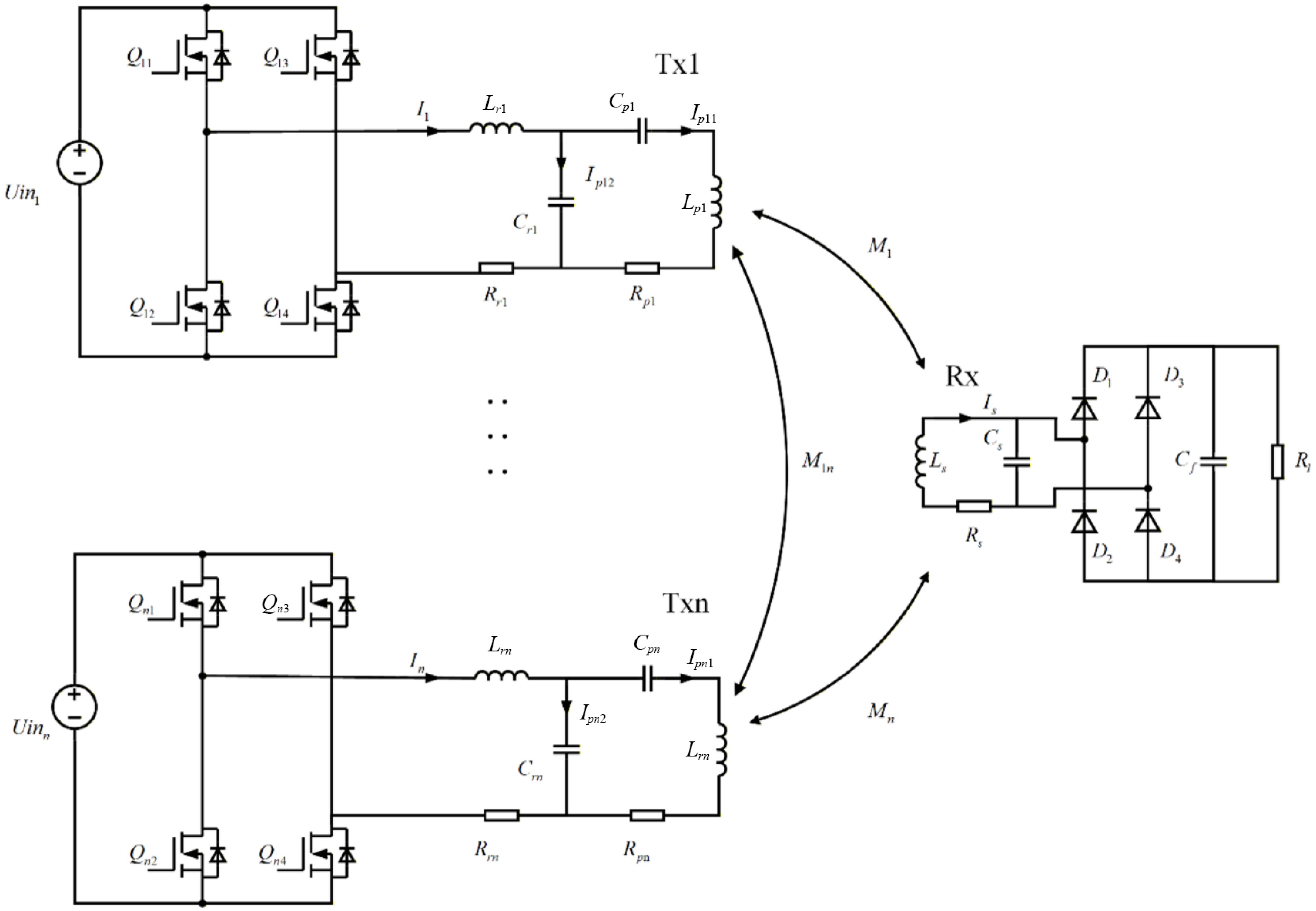
Figure 2.
MTA-WPT system circuit model.
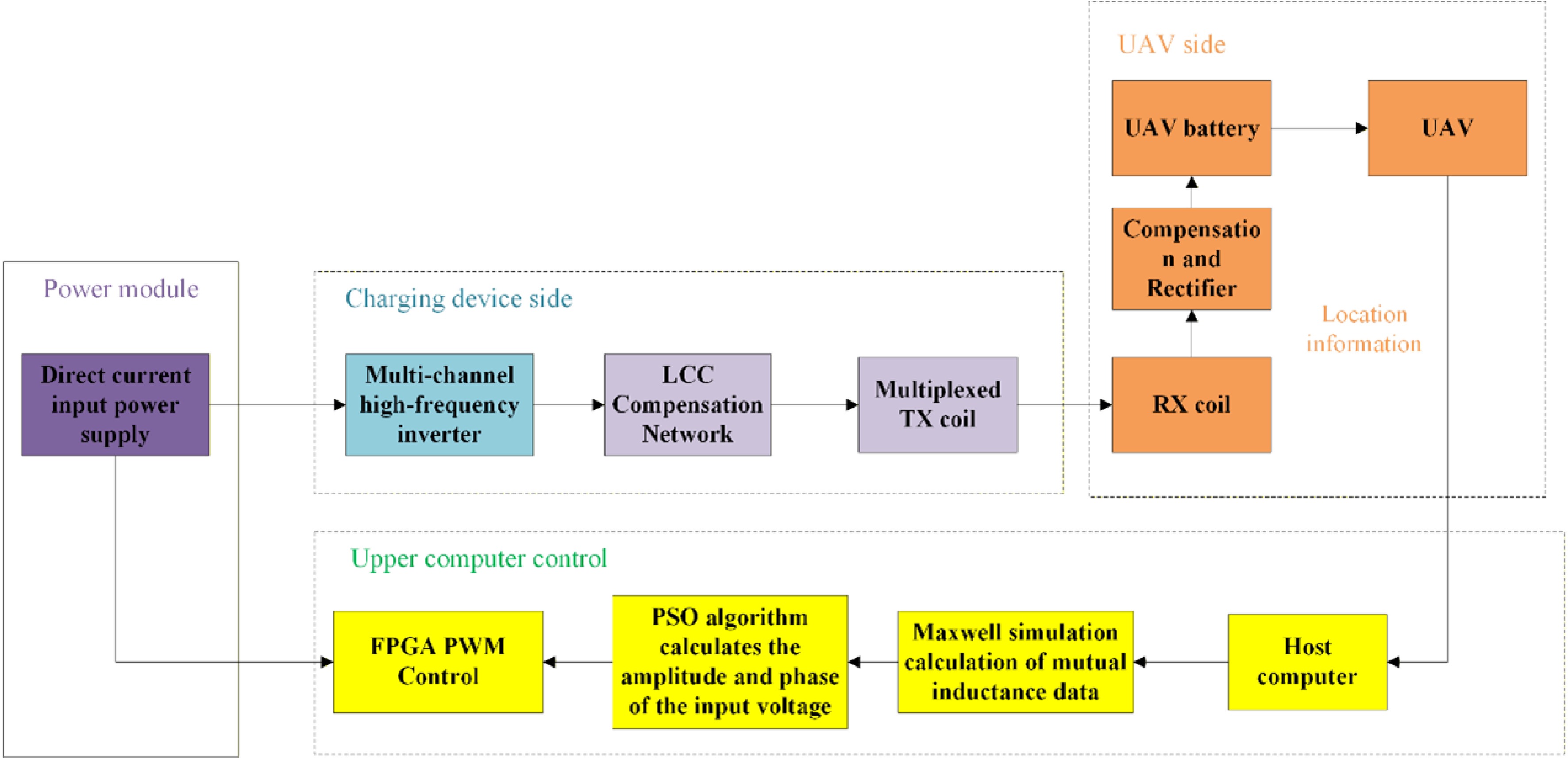
Figure 3.
Structure diagram of unmanned aerial vehicle charging system.
$ \begin{cases} Ui{n}_{1}=={I}_{1}(j\omega {L}_{r1}+{R}_{r1})+{I}_{p12}\dfrac{1}{j\omega {C}_{r1}}\\ {I}_{1}={I}_{p11}+{I}_{p12}\\ \dfrac{{I}_{p12}}{j\omega {C}_{r1}}={I}_{p11}\left(j\omega {L}_{p1}+\dfrac{1}{j\omega {C}_{p1}}+{R}_{p1}\right)-j\omega ({M}_{1}{I}_{s}+{M}_{12}{I}_{p21}+\cdots +{M}_{1n}{I}_{n1})\\ Ui{n}_{2}=={I}_{2}(j\omega {L}_{r2}+{R}_{r2})+{I}_{p22}\dfrac{1}{j\omega {C}_{r2}}\\ {I}_{2}={I}_{p21}+{I}_{p22}\\ \dfrac{{I}_{p22}}{j\omega {C}_{r2}}={I}_{p21}\left(j\omega {L}_{p2}+\dfrac{1}{j\omega {C}_{p2}}+{R}_{p2}\right)-j\omega ({M}_{21}{I}_{11}+{M}_{2}{I}_{s}+\cdots +{M}_{2n}{I}_{n1})\\ \cdots \\ Ui{n}_{\textit{n}}=={I}_{n}(j\omega {L}_{rn}+{R}_{rn})+{I}_{pn2}\dfrac{1}{j\omega {C}_{n1}}\\ {I}_{n}={I}_{pn1}+{I}_{pn2}\\ \dfrac{{I}_{p\mathrm{n}2}}{j\omega {C}_{rn}}={I}_{pn1}\left(j\omega {L}_{pn}+\dfrac{1}{j\omega {C}_{pn}}+{R}_{pn}\right)-j\omega ({M}_{n1}{I}_{11}+{M}_{n2}{I}_{p21}+\cdots +{M}_{n}{I}_{s})\\ \dfrac{{I}_{\text{s}}}{{Z}_{S}}=j\omega ({M}_{1}{I}_{11}+{M}_{2}{I}_{p21}+\cdots {M}_{n}{I}_{n1}) \end{cases} $ (1) where,
$ {I}_{n} $ $ {I}_{n1} $ $ {I}_{n2} $ $ {C}_{rn} $ $ {I}_{s} $ $ {Z}_{S} $ $ {Z}_{S} $ $ \begin{cases} {Z}_{cs}=\dfrac{1}{j\omega {C}_{s}}\\ {Z}_{p}=\dfrac{1}{\left(\dfrac{1}{{Z}_{cs}}+\dfrac{1}{{R}_{L}}\right)}\\ {Z}_{S}=j\omega {L}_{s}+{Z}_{p}+{R}_{s} \end{cases} $ (2) When the LCC-P compensation operates in resonance mode, its compensation network parameters satisfy:
$ \begin{cases} j\omega {L}_{rn}=-\dfrac{1}{j\omega {C}_{rn}}\\ j\omega ({L}_{pn}-{L}_{rn})=-\dfrac{1}{j\omega {C}_{pn}}\\ j\omega {L}_{s}=-\dfrac{1}{j\omega {C}_{s}} \end{cases} $ (3) In efficiency analysis, parasitic resistances of all components affect system performance. However, measured results show that the parasitic resistance of compensation capacitors is very small (approximately 1/10 that of compensation inductors) and can often be neglected. To analyze the relationship between system efficiency and mutual inductance among multiple coils, incorporating the parasitic resistance of the compensating inductor and the coil, becomes extremely complex. To simplify the efficiency analysis while capturing the influence of mutual inductances, we initially neglect the parasitic resistances of the compensation inductors and coils. Following the approach for a four-coil system[31], we extend the analysis to a five-coil LCC-P system. Assuming identical transmitter coil structures, the compensation network parameters are unified as:
$ {L}_{r} $ $ {C}_{r} $ $ {C}_{p} $ $ {I}_{n} $ $ {I}_{pn1} $ $ {I}_{pn2} $ $ {I}_{s} $ $ {P}_{out}=\dfrac{{R}_{L}{D}^{2}}{{L}_{r}{}^{2}{L}_{s}{}^{2}{\omega }^{2}} $ (4) $ {P}_{in}=\dfrac{{R}_{L}{D}^{2}+j{L}_{s}\omega {D}^{2}+j{L}_{s}{}^{2}\omega \displaystyle\sum \limits_{i=1}^{5}Ui{n}_{i}{S}_{i}}{{L}_{r}{}^{2}{L}_{s}{}^{2}{\omega }^{2}} $ (5) where,
$ \begin{cases} D={M}_{1}Ui{n}_{1}+{M}_{2}Ui{n}_{2}+{M}_{3}Ui{n}_{3}+{M}_{4}Ui{n}_{4}+{M}_{5}Ui{n}_{5}\\ S=\displaystyle\sum \limits_{j=1,j\neq i}^{5}{M}_{ij}Ui{n}_{j} \end{cases} $ (6) According to Formulas (4) and (5), the system efficiency is obtained as
$ EFF=\dfrac{{P}_{out}}{{P}_{in}}=\dfrac{{R}_{L}{D}^{2}}{{R}_{L}{D}^{2}+j{L}_{s}\omega {D}^{2}+j{L}_{s}{}^{2}\omega \displaystyle\sum \limits_{i=1}^{5}Ui{n}_{i}{S}_{i}} $ (7) Based on Formulas (4) and (7), if the system's compensation network and resonant frequency are fixed, the output power and efficiency of the five-coil system vary with changes in
$ D $ $ {R}_{L} $ If the compensation network of the system and the resonant frequency are determined, the output power and efficiency of the five-winding system will change with the variations of
$ D $ $ {R}_{L} $ Since the system is in resonance, the input voltage at resonance can be expanded as:
$ \begin{cases} Ui{n}_{1}=\dfrac{{A}_{1}}{\sqrt{2}}{e}^{j0}=\dfrac{{A}_{1}}{\sqrt{2}}\\ Ui{n}_{n}=\dfrac{{A}_{n}}{\sqrt{2}}{e}^{j{{\theta }_{n}}}=\dfrac{{A}_{n}}{\sqrt{2}}(\cos {\theta }_{n}+j\sin {\theta }_{n}) \end{cases} $ (8) where,
$ {A}_{n} $ $ {\theta }_{n} $ When the UAV hovers within the charging zone, its battery load remains within a fixed range and cannot be altered. The position of the receiving coil is fixed, thereby determining the mutual inductances between the receiver and transmitters. Therefore, the system's output power and efficiency can only be adjusted by modifying the input voltages
$ Ui{n}_{n} $ $ {A}_{n} $ $ {\theta }_{n} $ $ Ui{n}_{n} $ Multi-input coil amplitude allocation strategy
-
According to Li et al.[32], under ideal conditions for optimal efficiency in a two-coil system, the relationship between current magnitudes is:
$ {I}_{p21}=x{I}_{p11} $ $ x={M}_{2}/{M}_{1} $ $ {I}_{pn1}=\dfrac{Ui{n}_{n}}{j\omega Lr} $ (9) With constant compensation parameters, the current magnitude is linearly related to the input voltage. Hence, the optimal voltage ratio for two coils is:
$ Ui{n}_{2}=xUi{n}_{1} $ (10) According to Pang et al.[31], the condition for achieving optimal efficiency in a four-coil system with LCC-S compensation is the following relationship between the input current magnitude:
$ \begin{cases} {I}_{p21}=x{I}_{p11}\\ {I}_{p31}=y{I}_{p11}\\ {I}_{p41}=z{I}_{p11} \end{cases} $ (11) where,
$ x={M}_{2}/{M}_{1} $ $ y={M}_{3}/{M}_{1} $ $ z={M}_{4}/{M}_{1} $ $ Ui{n}_{2}=xUi{n}_{1} $ $ Ui{n}_{3}=yUi{n}_{1} $ $ Ui{n}_{4}=zUi{n}_{1} $ $ Ui{n}_{5}=vUi{n}_{1} $ $ EFF=\dfrac{{C}_{1}{A}^{2}}{{C}_{2}B+{C}_{3}{A}^{2}} $ (12) where,
$ {C}_{1} $ $ {C}_{2} $ $ {C}_{3} $ $ {L}_{s} $ $ \omega $ $ {R}_{s} $ $ {R}_{rn} $ $ {R}_{pn} $ $ A={M}_{1}+{M}_{2}x+{M}_{3}y+{M}_{4}z+{M}_{5}v $ $ B=1+{x}^{2}+{y}^{2}+{z}^{2}+{v}^{2} $ $ x $ $y $ $z $ $v $ $ \begin{cases} x=\dfrac{{M}_{2}}{{M}_{1}}\\ y=\dfrac{{M}_{3}}{{M}_{1}}\\ z=\dfrac{{M}_{4}}{{M}_{1}}\\ v=\dfrac{{M}_{5}}{{M}_{1}} \end{cases} $ (13) This indicates that, with fixed phases and system structure, optimal efficiency requires the input voltage amplitudes to be proportional to the respective mutual inductances. This conclusion holds for five-coil and general multi-coil structures.
Analysis of multi-input coil structure
-
The receiver coil size is determined by the UAV landing gear structure. Both transmitter and receiver coils are chosen as 20 × 20 cm squares. Simulations in ANSYS Electronics/Maxwell show that when all Tx coils are activated simultaneously, cross-coupling occurs among them. According to Formula (5), this increases the reactive power input to the system, degrading charging performance. As documented by Kang et al.[33], a specific lateral offset distance exists where cross coupling between two receiver coils becomes zero; a diagonal offset distance also eliminates cross coupling. However, in a four-coil configuration, overlapping cannot simultaneously nullify cross coupling for all four coils. Therefore, overlapping is used to minimize cross coupling as much as possible. Although overlapping reduces the effective charging area of the system compared to a non-overlapping configuration, it reduces the mutual inductance between adjacent Tx coils to nearly zero, significantly minimizing reactive circulating currents caused by cross-coupling. This enables the system to deliver more energy to the receiver, thereby improving system efficiency. Additionally, the overlapping coil configuration results in a more uniform magnetic field distribution, avoiding localized charging dead zones, which helps the UAV obtain relatively stable charging conditions at different landing positions. Maxwell simulations indicate that the zero cross-coupling lateral offset distance is 3.75 cm, which is selected as the spacing between adjacent transmitter coils for simulation and experimental testing.
Figure 4a, b displays the magnetic field distributions of four-coil and five-coil arrays, respectively. Analysis reveals that the four-coil array exhibits lower magnetic field strength at the center and significant field inhomogeneity, resulting in charging dead spots. Therefore, the five-coil array is selected for charging experiments. Figure 5 demonstrates how varying the phases of transmitter coil currents can concentrate the magnetic field in specific regions. For example, Fig. 5b concentrates the field above Tx3, while Fig. 5c concentrates it at the junction of Tx3, Tx4, and Tx5. As shown in the figure above, analyzing the phase effect on the current in the receiving coil through the magnetic field angle is relatively challenging.
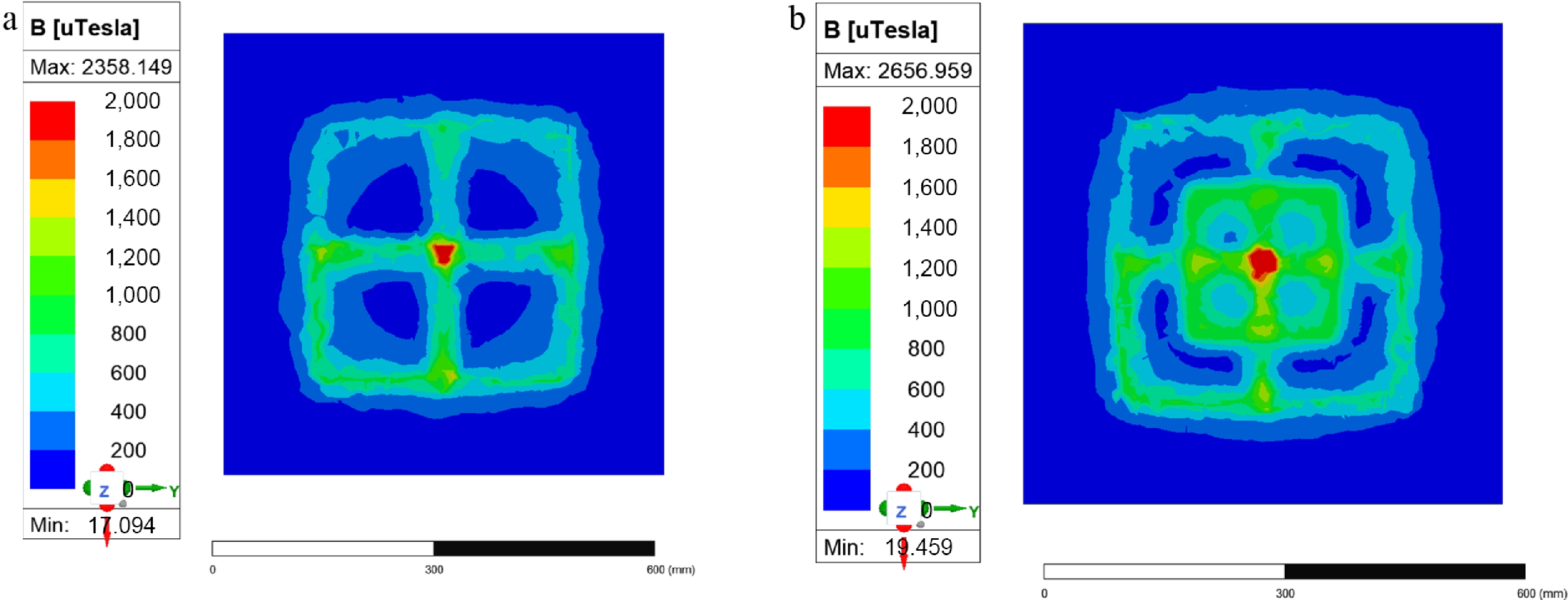
Figure 4.
(a) Simulation diagram of four-coil magnetic field strength. (b) Simulation diagram of five-coil magnetic field strength.
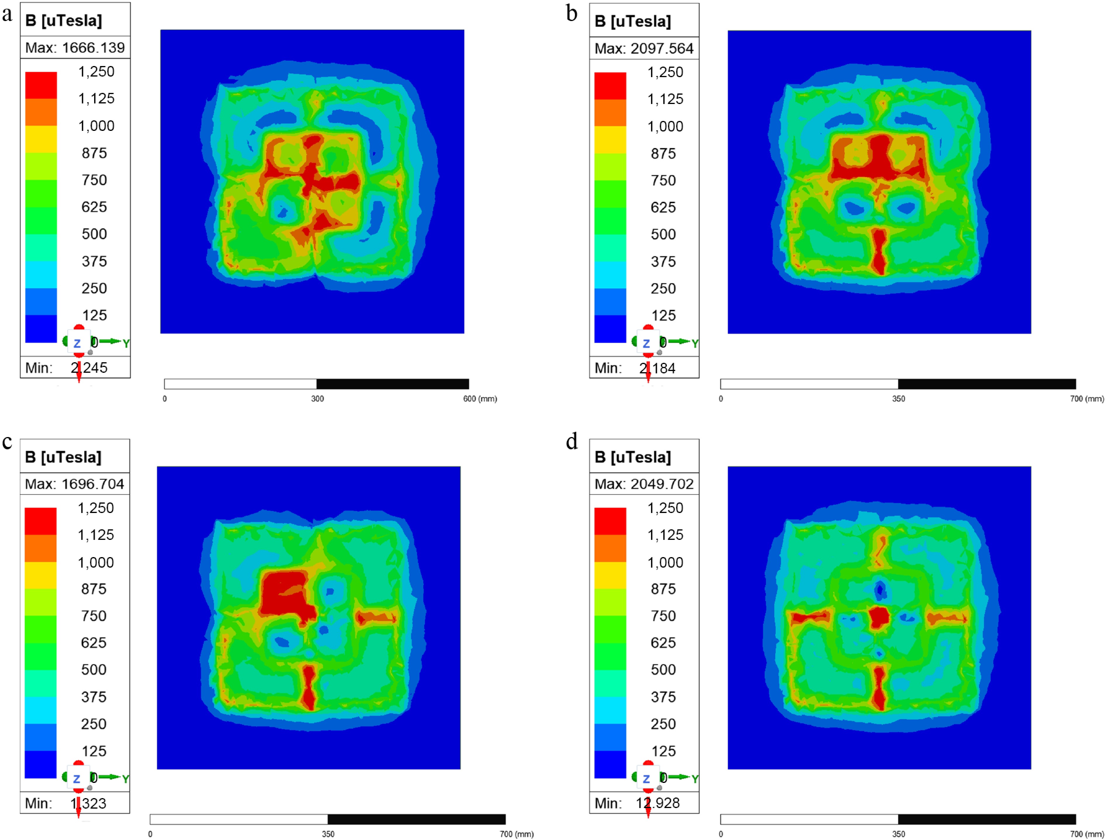
Figure 5.
(a) Tx1 is offset by 180°. (b) Tx1 and Tx2 are offset by 180°. (c) Tx1, Tx2, and Tx3 are offset by 180°. (d) Tx1, Tx2, Tx3, and Tx4 are offset by 180°.
Figure 6 shows a comparison between the simulated mutual inductance values of the receiver coil and the five transmitter coils in the five-coil array (ANSYS Electronics/Maxwell) and the actual measured values. The simulation results closely match the experimental measurements. The simulation software can be used to model the mutual inductance values between the receiver coil and transmitter coils during an actual UAV landing and perform calculations.
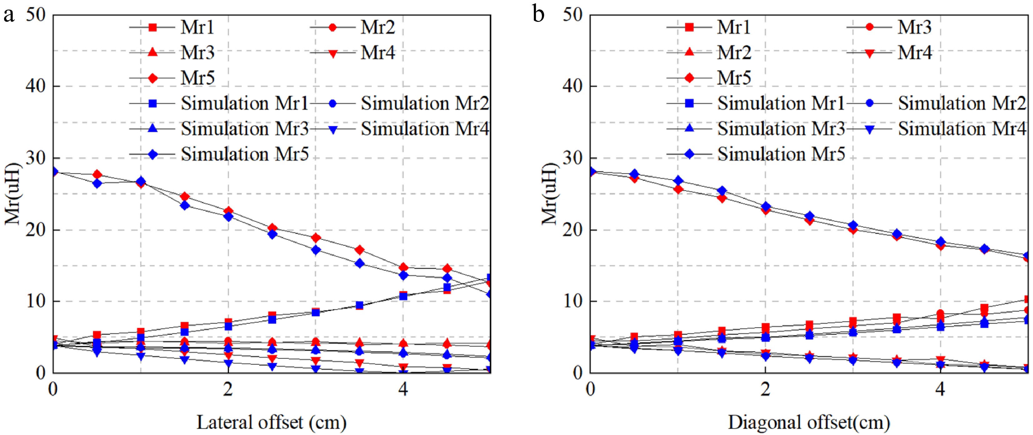
Figure 6.
The mutual inductance experiment and simulation results between the receiving coil and the five-antenna coil: (a) Lateral offset mutual inductance diagram, (b) diagonal offset mutual inductance diagram.
Multi-input coil amplitude and phase optimization algorithm
-
The model indicates that all components in the MTA-WPT system are linear elements, and the system's transmitter source is unaffected by circuit devices. Therefore, it can be regarded as a linear system and equivalently simplified into a multiport network model. This network retains only the input voltage source and receiving resistor, establishing the relationship between its input and output ports to better analyze the input-output response relationship.
According to Formula (8), it is evident that adjusting the phase of the input voltage can alter the overall system efficiency. For a multi-input single-output system, the relationship between the receiving-end voltage and the output-end voltage is given by:
$ {I}_{L}={\dot{A}}_{1}{e}^{j{{\dot{\theta }}_{1}}}+{\dot{A}}_{2}{e}^{j{{\dot{\theta }}_{2}}}+\cdots +{\dot{A}}_{n}{e}^{j{{\dot{\theta }}_{n}}} $ (14) where,
$ {\dot{A}}_{n} $ $ {\dot{\theta }}_{n} $ Particle swarm optimization algorithm
-
This paper employs the PSO algorithm to determine maximum efficiency by adjusting the phase and amplitude of the system's input voltage. The algorithm updates the particle swarm using the following Formulas (15) and (16):
$ {x}_{n}(i)={x}_{n}(i-1)+{v}_{n}(i) $ (15) $ \begin{split}{v}_{n}(i)=\;&w(i){v}_{n}(i-1)+{c}_{1}{r}_{1}[pbes{t}_{n\max }(i-1)-{\mathrm{x}}_{n}(i-1)]\\ &+{c}_{2}{r}_{2}[gbes{t}_{\max }(i-1)-{\mathrm{x}}_{n}(i-1)] \end{split}$ (16) Among these,
$ {x}_{n}(i) $ $ i $ $ {v}_{n}(i) $ $ i $ $ pbes{t}_{n\max }(i) $ $ i $ $ gbes{t}_{\max }(i) $ $ i $ $ {c}_{1} $ $ {c}_{2} $ $ {r}_{1} $ $ {r}_{2} $ $ w(i) $ $ i $ 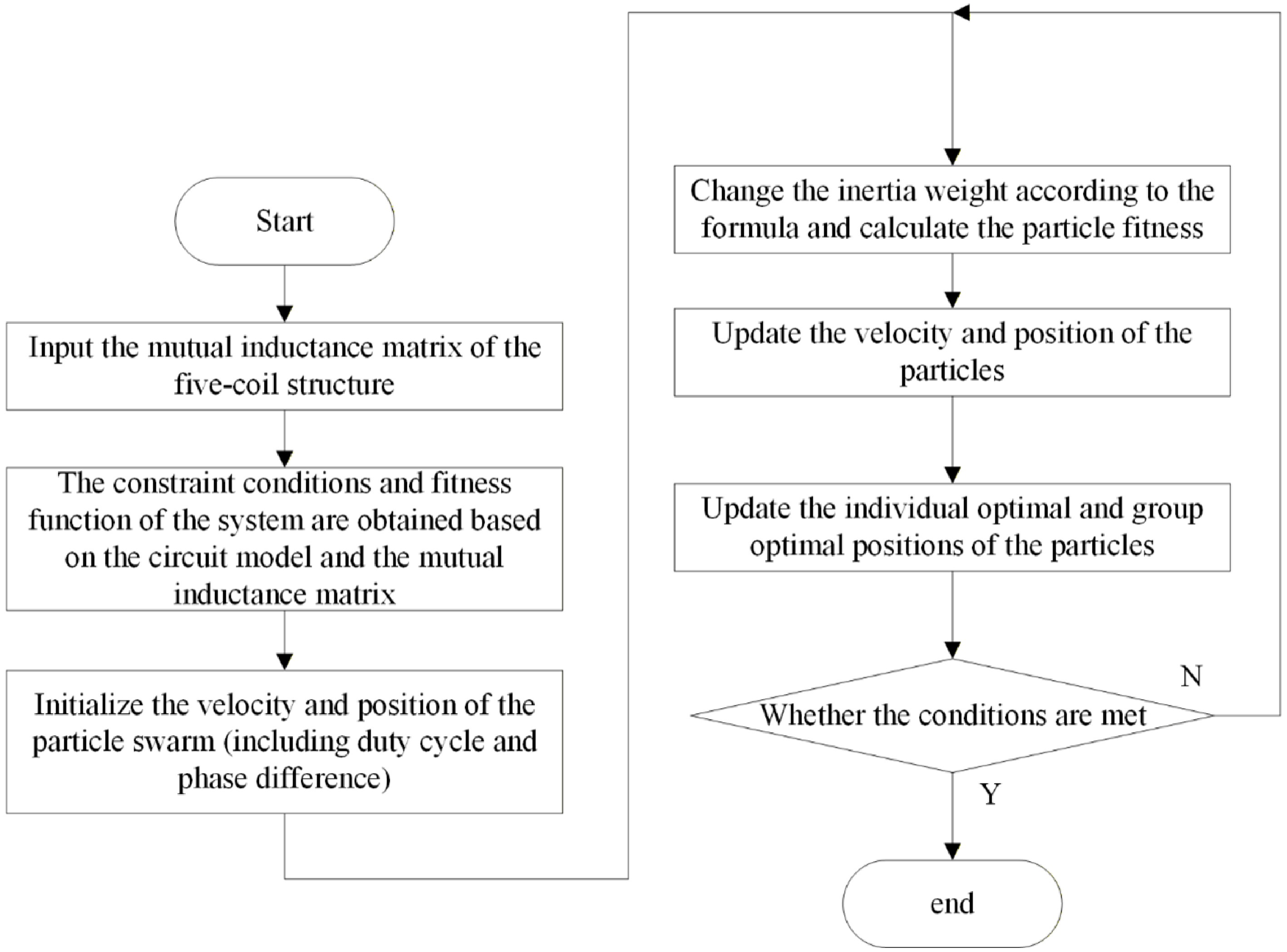
Figure 7.
Specific implementation steps of the particle swarm algorithm.
Analysis of algorithm parameters and their values
-
During algorithm execution, the inertia weight factor gradually decreases with each iteration to limit particle velocity and prevent them from getting stuck in local optima. When
$ w $ $ w $ $ w(i)=\max (0.4,0.9w(i-1)) $ (17) From Formula (17), it can be seen that
$ {w}_{\max } $ $ {w}_{\min } $ $ {c}_{1} $ $ {c}_{2} $ $ {c}_{1} $ $ {c}_{2} $ $ {c}_{1} $ $ {c}_{2} $ The optimization objective of this multi-coil model is constrained by the achievable output power of the system. Consequently, employing a penalty function to address constrained optimization is a common approach. This method transforms complex constraints into simpler unconstrained optimization problems by introducing a penalty term in the objective function. Solutions violating constraints incur penalties, and if the search direction contradicts the constraints, the penalty coefficient in the penalty function gradually increases. Solutions violating constraints incur progressively greater penalties, thereby gradually satisfying constraints during optimization.
From the above analysis, the primary physical constraints for this optimization are:
$ \begin{cases} Ui{n}_{n} \lt \max \_ Uin\\ Pi{n}_{n} \gt 0 \end{cases} $ (18) To handle the equality constraints in Formula (18), this paper adopts the exterior penalty function method. The basic idea is that when a search particle is outside the feasible region, a penalty term is introduced into the objective function. This penalty term increases sharply as the degree of constraint violation intensifies, thereby forcing the optimization process to approach the feasible region. Based on this, the fitness expression of the penalty function is:
$ F(x)=f(x)+\mu \mathrm{T }(x) $ (19) Therefore, the penalty function is defined as:
$ \begin{cases} f=f-penalt{y}_{1}\max (0,Ui{n}_{n}-\max \_ Uin)\\ f=f-penalt{y}_{2}\max (0,0-Pin) \end{cases} $ (20) where,
$ f $ $ penalt{y}_{1} $ $ penalt{y}_{2} $ To ensure the system output power remains at a fixed value, a Gaussian function is employed to reward solutions closer to the target power. Specifically, solutions near the target power exhibit higher fitness, while those farther from the target power have lower fitness.
$ {f}_{p}={e}^{-{{\left(\tfrac{{P}_{out}-T\arg et\_ powe\mathrm{r}}{T\arg et\_ power}\right)}^{2}}} $ (21) While ensuring the output power, guarantee the efficiency of the system
$ f={h}_{1}{f}_{p}+{h}_{2}{f}_{eff} $ (22) Here,
$ {f}_{p} $ $ {f}_{eff} $ $ T\;\arg\; et\_ power $ $ {h}_{1} $ $ {h}_{2} $ -
To validate the theoretical analysis, a prototype five-transmitter-coil WPT system was built. The setup includes five inverters, five LCC compensation networks, five transmit coils, one receive coil, secondary compensation, and rectifiers. The inverters drive MOSFETs (FDH055N15A) via IR2104 controllers. The PWM signals are generated by an FPGA (xc7z020clg400-2), allowing adjustment of duty cycle and phase difference between inverters. The LCC compensation network uses PQ-2918 inductors and CCB capacitors. The receiver rectifier consists of four ES3B-E3/57T fast-recovery diodes. The system operates at a 24 V input and 100 kHz. Detailed parameters are listed in Table 1. The mutual inductance M matrix under the condition of 5 cm lateral offset is listed in Table 2, which shows the lateral offset in the x-axis. Here,
$ {L}_{1} $ $ {L}_{5} $ $ {L}_{6} $ $ {M}_{1} $ $ {M}_{5} $ $ {M}_{ij} $ $ 1\leq i\leq 5 $ $ 1\leq j\leq 5 $ $ i $ $ j $ Table 1. MTA-WPT system parameters.
Parameter Experiment value Parameter Experiment value $ Uin $ 24 V $ {L}_{s} $ 37 μH $ f $ 100 kHz $ {C}_{s} $ 64.7 nF $ {L}_{r} $ 15 μH $ {R}_{r} $ 145 m$ \Omega $ $ {C}_{r} $ 163 nF $ {R}_{p} $ 236 m$ \Omega $ $ {C}_{p} $ 110 nF $ {R}_{s} $ 236 m$ \Omega $ $ {L}_{p} $ 37 μH $ {R}_{l} $ 130 $ \Omega $ Table 2. The mutual inductance M matrix under the condition of a 5 cm lateral offset.
Self-inductance and mutual inductance $ {L}_{1} $ $ {M}_{12} $ $ {M}_{13} $ $ {M}_{14} $ $ {M}_{15} $ $ {M}_{1} $ $ {M}_{21} $ $ {L}_{2} $ $ {M}_{23} $ $ {M}_{24} $ $ {M}_{25} $ $ {M}_{2} $ $ {M}_{31} $ $ {M}_{32} $ $ {L}_{3} $ $ {M}_{34} $ $ {M}_{35} $ $ {M}_{3} $ $ {M}_{41} $ $ {M}_{42} $ $ {M}_{43} $ $ {L}_{4} $ $ {M}_{45} $ $ {M}_{4} $ $ {M}_{51} $ $ {M}_{52} $ $ {M}_{53} $ $ {M}_{54} $ $ {L}_{5} $ $ {M}_{5} $ $ {M}_{1} $ $ {M}_{2} $ $ {M}_{3} $ $ {M}_{4} $ $ {M}_{5} $ $ {L}_{6} $ Self-inductance and mutual inductance values 37.0863 0.621815 0.461625 1.866375 4.252525 10.3442 0.621815 39.8564 2.363775 0.5875 4.2872 0.747275 0.461625 2.363775 37.1706 0.439625 4.222975 8.8188 1.866375 0.5875 0.439625 37.4132 4.6258 0.83975 4.252525 4.2872 4.222975 4.6258 38.4432 16.01258 10.3442 0.747275 8.8188 0.83975 16.01258 36.6945 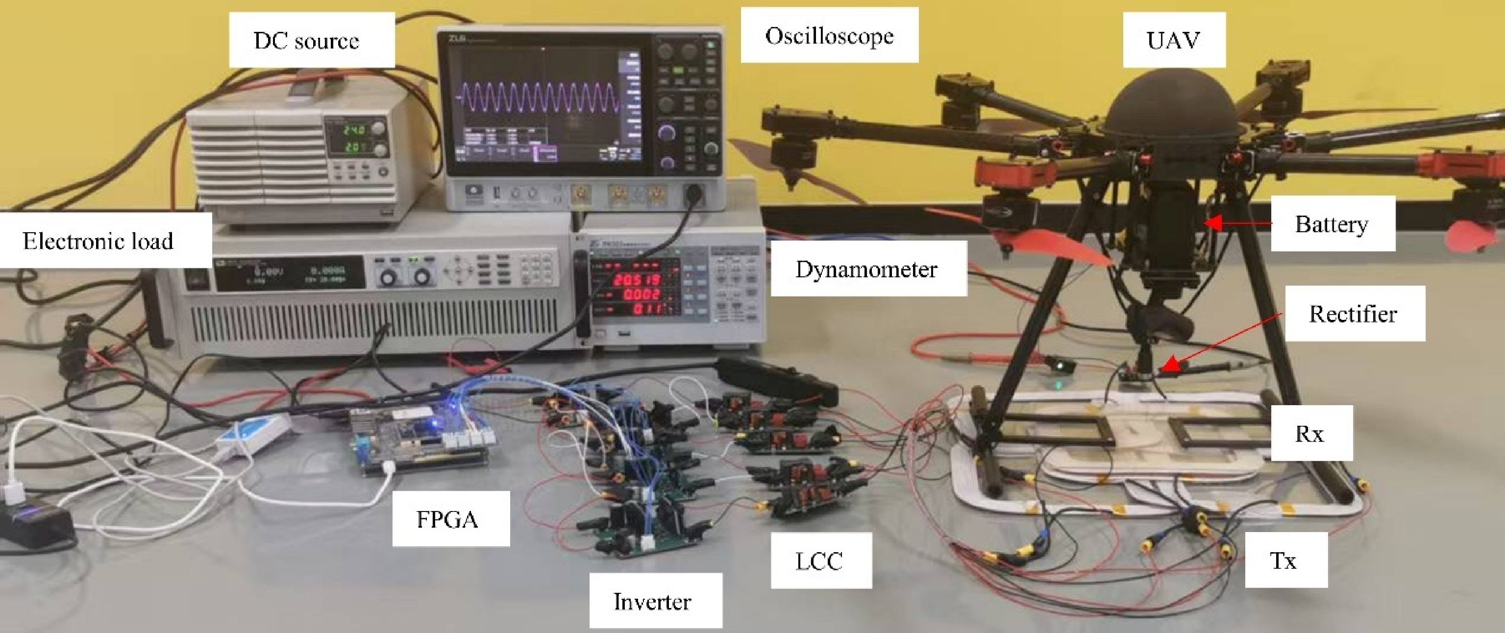
Figure 8.
MTA-WPT system experimental prototype.
Experimental results
-
To verify that the experimental prototype can still achieve charging when the RX coil is in an offset position, the starting position was set with the RX coil centered within the five-coil array, with a Z-axis distance of 1 cm. When the input DC voltages were all set to 24 V without amplitude or phase control, Output power was measured for the RX coil at horizontal offsets of 5 cm and diagonal offsets of 5 cm relative to the center position under various impedance conditions. Due to the symmetry of the multi-coil structure, experimental data were collected for only one direction of horizontal and diagonal offset. At a load impedance of 15
$ \Omega $ 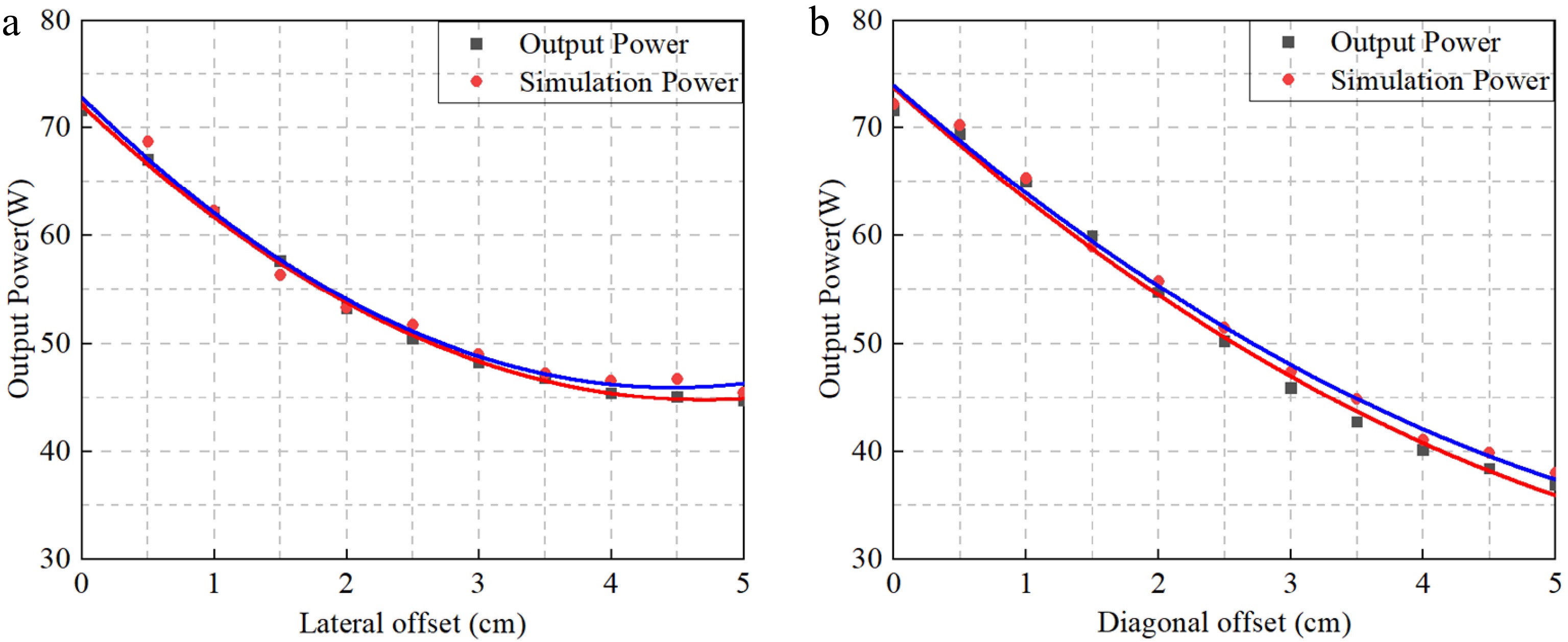
Figure 9.
Comparison of simulated and measured output power: (a) lateral offset; (b) diagonal offset.
The voltage/current waveforms of the inverter, input coil, output coil, and load under a 5 cm lateral offset were measured using oscilloscopes ZDS5054Pro (ZLG) and DSOX3022T (Keysight), as shown in Figs 10−15.
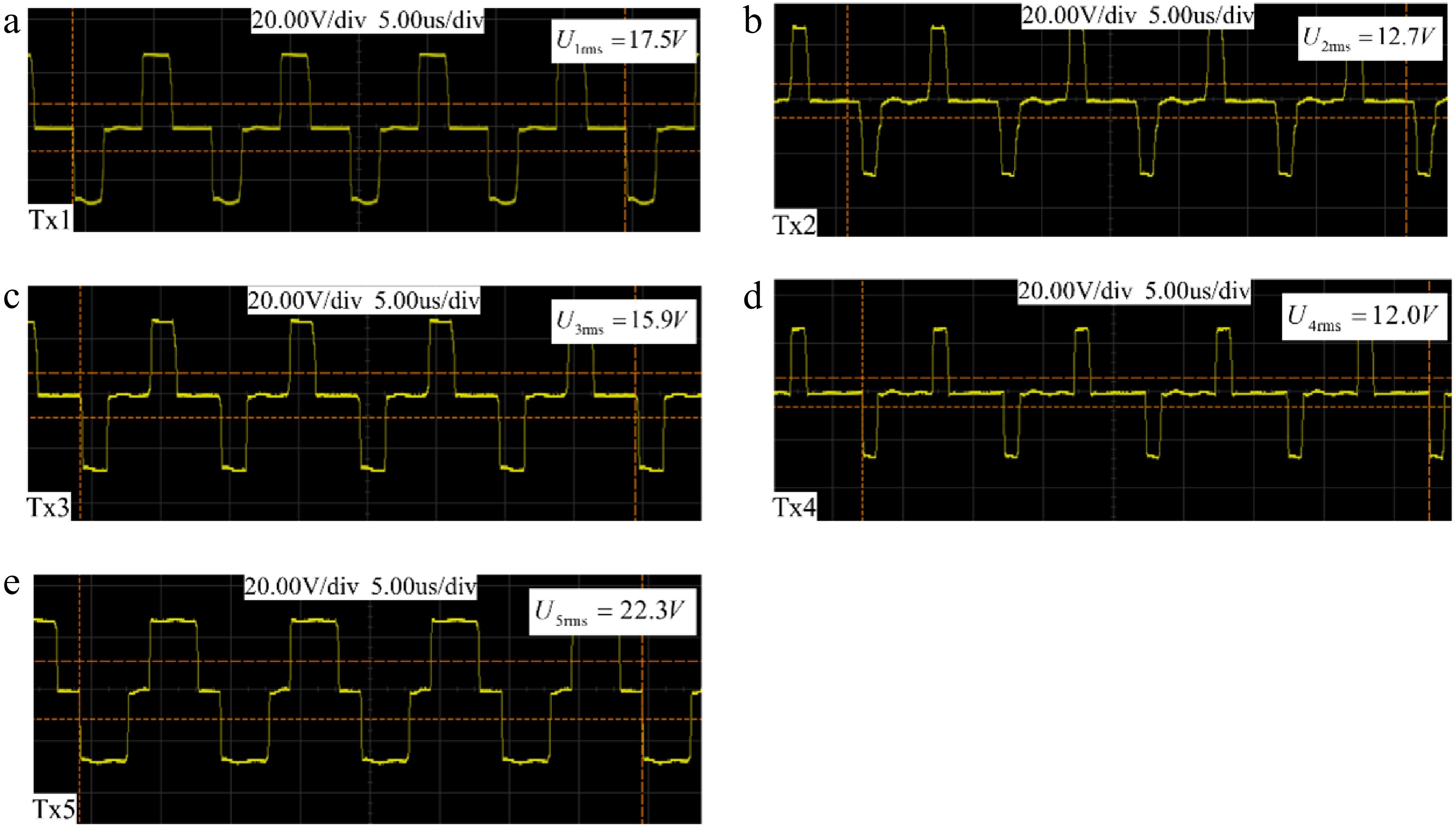
Figure 10.
Output voltages of the five-channel inverters. (a) Tx1. (b) Tx2. (c) Tx3. (d) Tx4. (e) Tx5.
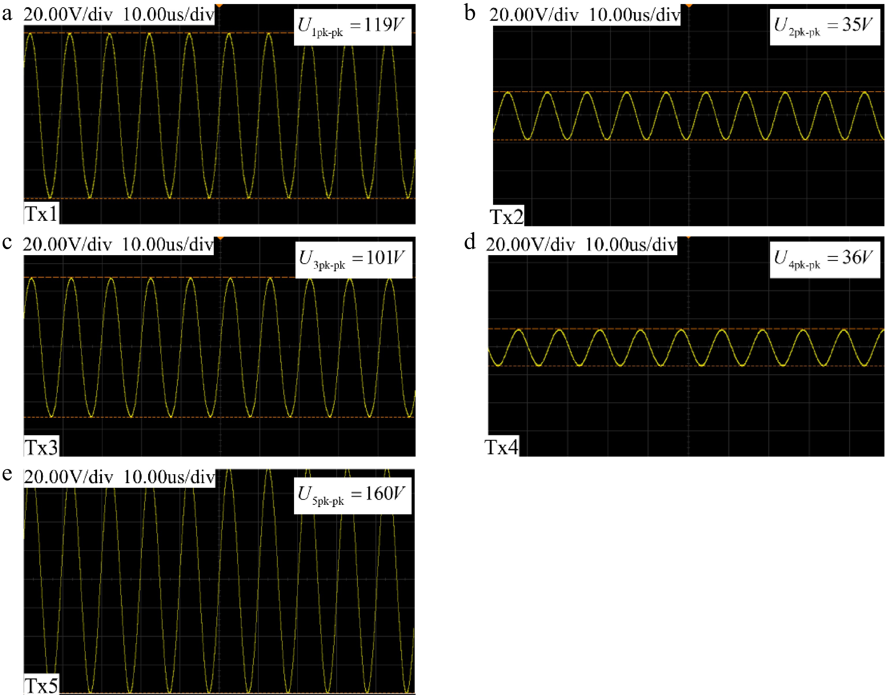
Figure 11.
Input voltage of the five-channel Tx coil. (a) Tx1. (b) Tx2. (c) Tx3. (d) Tx4. (e) Tx5.
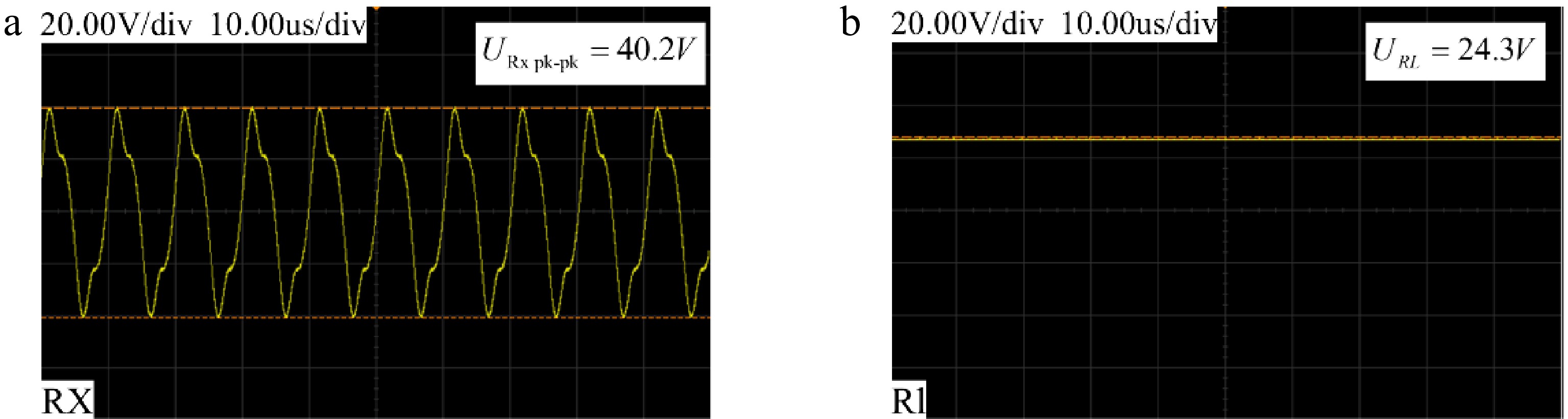
Figure 12.
(a) Output voltage of the Rx coil; (b) Input voltage of the load.
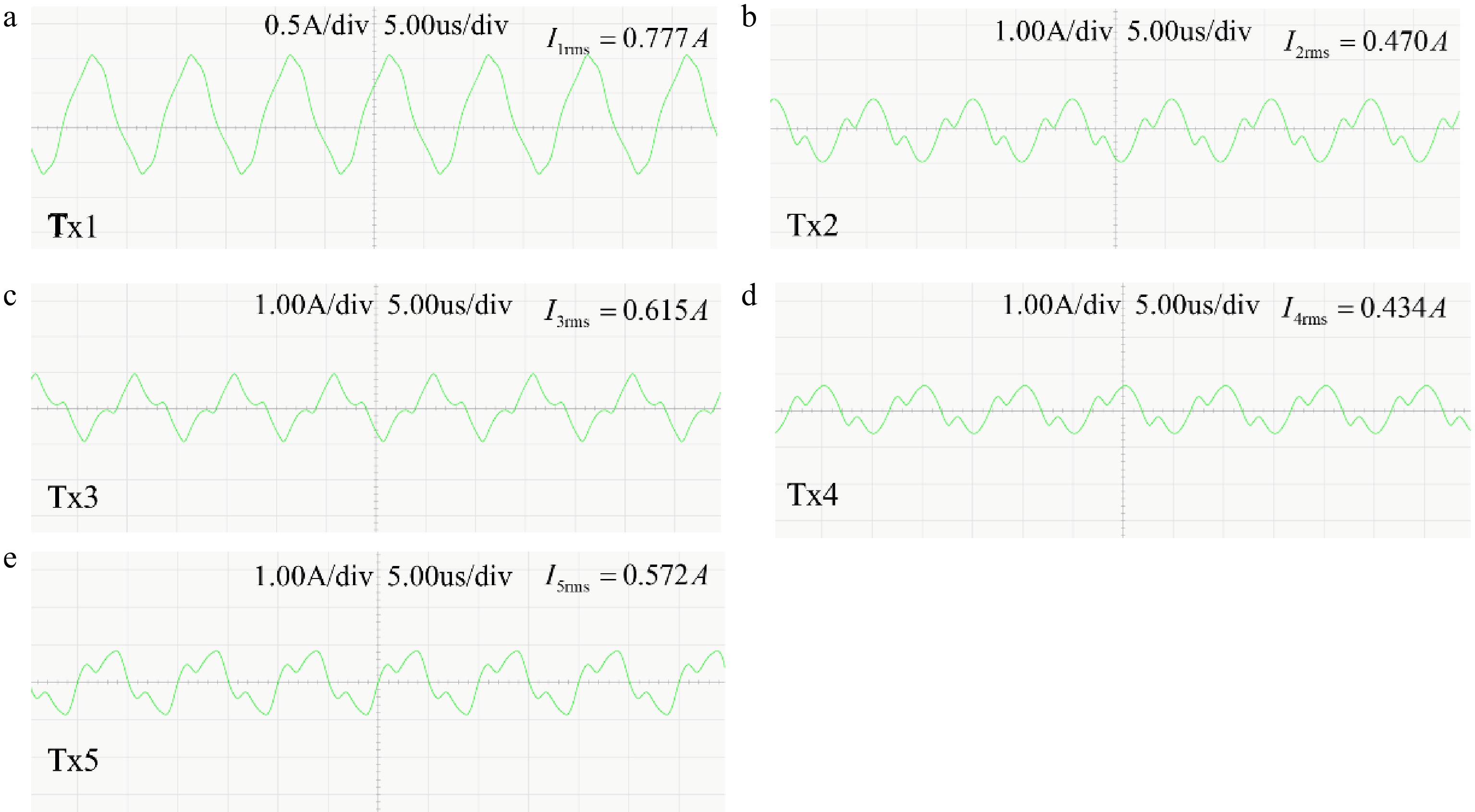
Figure 13.
Output currents of the five-channel inverters. (a) Tx1. (b) Tx2. (c) Tx3. (d) Tx4. (e) Tx5.
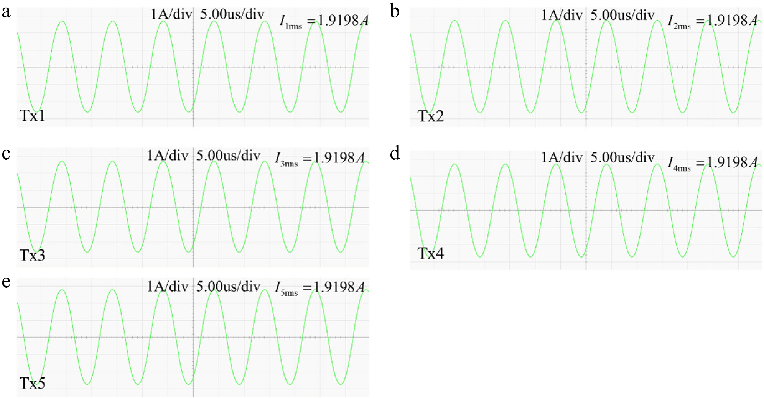
Figure 14.
Input currents of the five-channel Tx coil. (a) Tx1. (b) Tx2. (c) Tx3. (d) Tx4. (e) Tx5.
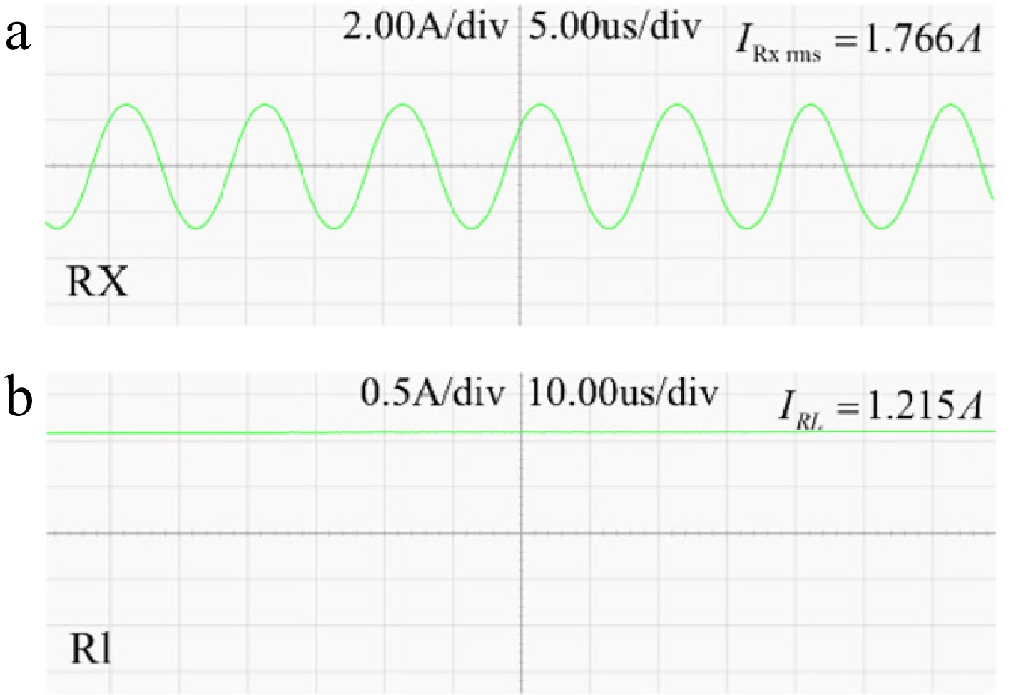
Figure 15.
(a) Output current of the Rx coil; (b) Input current of the load.
To validate the system's constant current output performance, load current changes were captured using a PA323 power meter (ZLG), changes from 5 to 10, and then to 20
$ \Omega $ 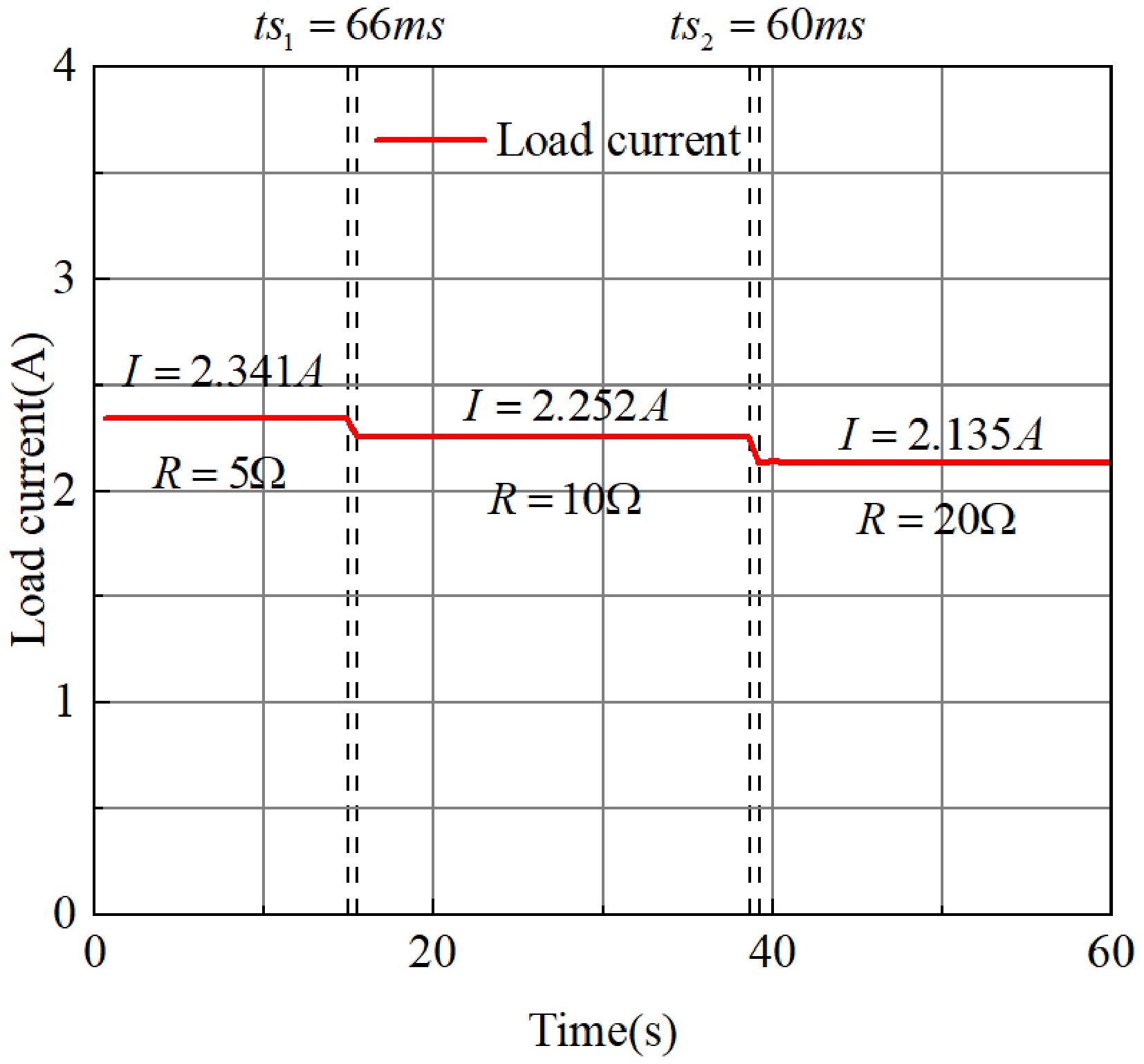
Figure 16.
The load current varies with the load.
Simulation and experimental analysis of the particle swarm optimization algorithm
-
Using Simulink software, a circuit model of the multi-coil coupled transmission system was constructed. The circuit parameters of the system are shown in Table 1. Through joint simulation with MATLAB and Simulink, the system's optimal efficiency under fixed power was optimized. With the default phase of Tx1 coil set to 0, the phase difference between each subsequent coil and its preceding coil was defined as its input variable. The respective inputs were:
$ {\theta }_{12} $ $ {\theta }_{23} $ $ {\theta }_{34} $ $ {\theta }_{45} $ $ {\theta }_{12} $ $ {\theta }_{23} $ $ {\theta }_{34} $ $ {\theta }_{45} $ $ {D}_{c} $ $ {D}_{c} $ Table 3. Algorithm parameter settings.
Parameter Parameter value Position variables (including four phase differences and duty ratios) –90°~90°; 0.05~0.5 Number of particles $ N $ 50 Number of iterations iter 100 Speed variable $ v $ −5~5; −0.02~0.02 Inertia weight $ w $ 0.4~0.9 Learning factor $ {c}_{1} $, $ {c}_{2} $ 1.5 Proportional coefficient $ {h}_{1} $, $ {h}_{2} $ 0.75, 0.25 Penalty coefficient $ penalt{y}_{1} $, $ penalt{y}_{2} $ 0.05, 0.1 Similarly, with the RX coil centered in the four-coil array as the starting position, simulations were conducted to optimize output power and efficiency under different impedance conditions when the RX coil was horizontally offset by 5 cm and diagonally offset by 5 cm relative to the center position. This analysis compared power and efficiency with and without the search algorithm. The experimental results are shown in Fig. 17.
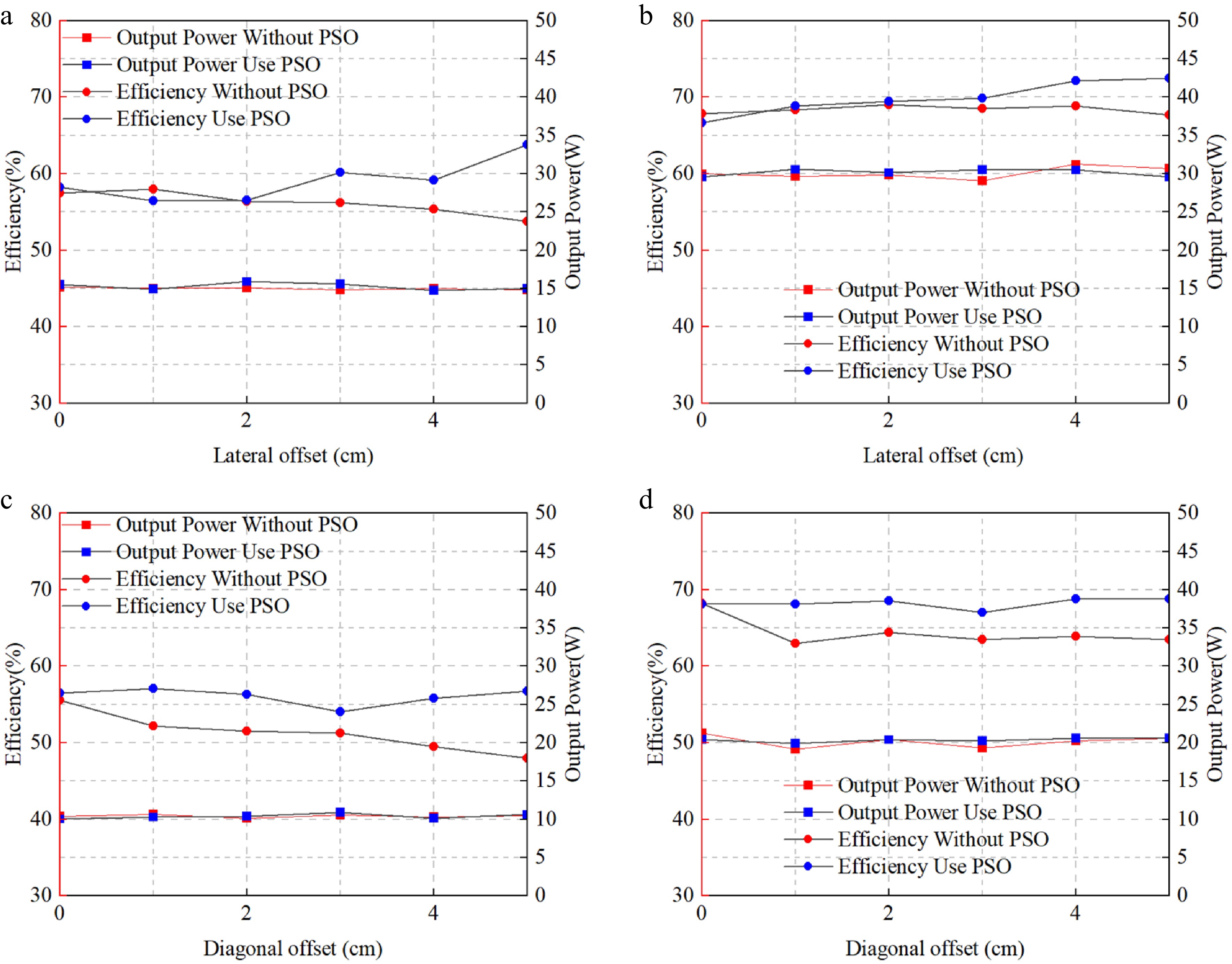
Figure 17.
(a) Efficiency curve at 15 W with 10 $ \Omega $ Load and 5 cm horizontal offset. (b) Efficiency curve at 30 W with 20 $ \Omega $ load and 5 cm horizontal offset. (c) Efficiency curve at 10 W with 10 $ \Omega $ load and 5 cm diagonal offset. (d) Efficiency curve at 20 W with 20 $ \Omega $ Load and 5 cm diagonal offset.
As shown in Fig. 17, Fig. 17a, b, under lateral displacement conditions, the algorithm maintains comparable charging efficiency to the non-algorithm approach during the initial displacement phase while maintaining stable power output. However, as displacement distance increases, the algorithm progressively enhances system efficiency. Fig. 17c, d illustrates diagonal displacement scenarios. Under stable-power conditions, the algorithm significantly enhances system efficiency across the entire displacement range. For a load of 20
$ \Omega $ Table 4. Efficiency comparison under horizontal offset.
Offset distance (cm) Efficiency without PSO
for 10 $ \Omega $ (%)Efficiency use PSO for 10 $ \Omega $ (%) Efficiency without PSO for 20 $ \Omega $ (%) Efficiency use PSO for 20 $ \Omega $ (%) 0 57.4933 58.23086 67.85213 66.66081 1 57.989 56.47121 68.33018 68.84291 2 56.35397 56.53843 69.02037 69.42831 3 56.19405 60.18519 68.50459 69.87048 4 55.33274 59.14359 68.86572 72.12933 5 53.75083 63.80204 67.68607 72.51287 Output power (W) 15 15 30 30 Table 5. Efficiency comparison under diagonal offset.
Offset distance (cm) Efficiency without PSO for 10 $ \Omega $ (%) Efficiency use PSO for 10 $ \Omega $ (%) Efficiency without PSO for 20 $ \Omega $ (%) Efficiency use PSO for 20 $ \Omega $ (%) 0 55.59878 56.5317 68.22239 68.14133 1 52.20701 57.12194 62.98619 68.1694 2 51.52683 56.29865 64.40019 68.58894 3 51.25058 54.06424 63.50154 67.0334 4 49.53487 55.81579 63.8911 68.78317 5 48.01168 56.78205 63.4688 68.78317 Output power (W) 10 10 20 20 UAV constant current charging experiment
-
To validate the charging performance of the UAV battery, charging experiments were conducted. The battery pack has a full voltage of 22.2 V. Wireless charging input was set to 32 V to achieve 1.5 A constant current and charging at approximately 30 W. The UAV was positioned at the center, with a lateral offset of 5 cm, and with a diagonal offset of 5 cm for charging tests. The charging voltage and current at a diagonal offset of 5 cm are shown in Fig. 18.
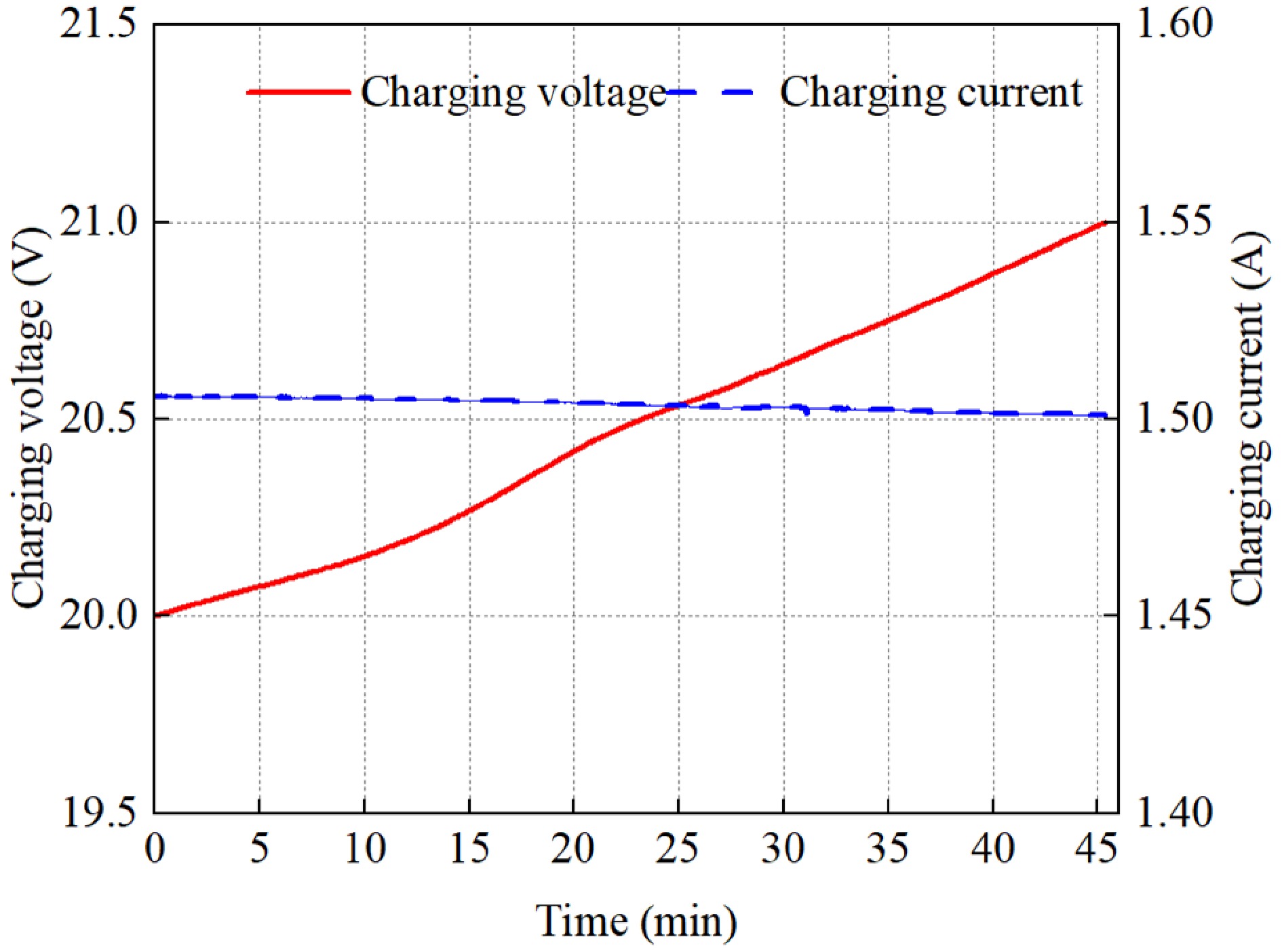
Figure 18.
The charging voltage and current under a 5 cm diagonal offset.
During the 46-min charging cycle with a 5 cm diagonal offset, the charging current remained essentially constant at approximately 1.5 A. The battery voltage increased from 20 to 21 V, with charging power maintaining around 30 W. This demonstrates that even with system displacement, the LCC-P topology enables the system to maintain a constant charging current. Consequently, charging curves at other system positions exhibit similar characteristics to those shown in Fig. 18.
As shown in Figs 19−21, the algorithm slightly improves system efficiency when the receiver coil is centered. However, when the receiver coil is significantly offset from the center, system efficiency increases substantially-a result consistent with electronic load experiments. At a charging power of approximately 30 W, maximum efficiency rose from 57.56% to 67.72%, representing a 10.16% improvement. In summary, the system employs a multi-transmitter coil configuration with the algorithm to achieve high-efficiency charging of UAV batteries.
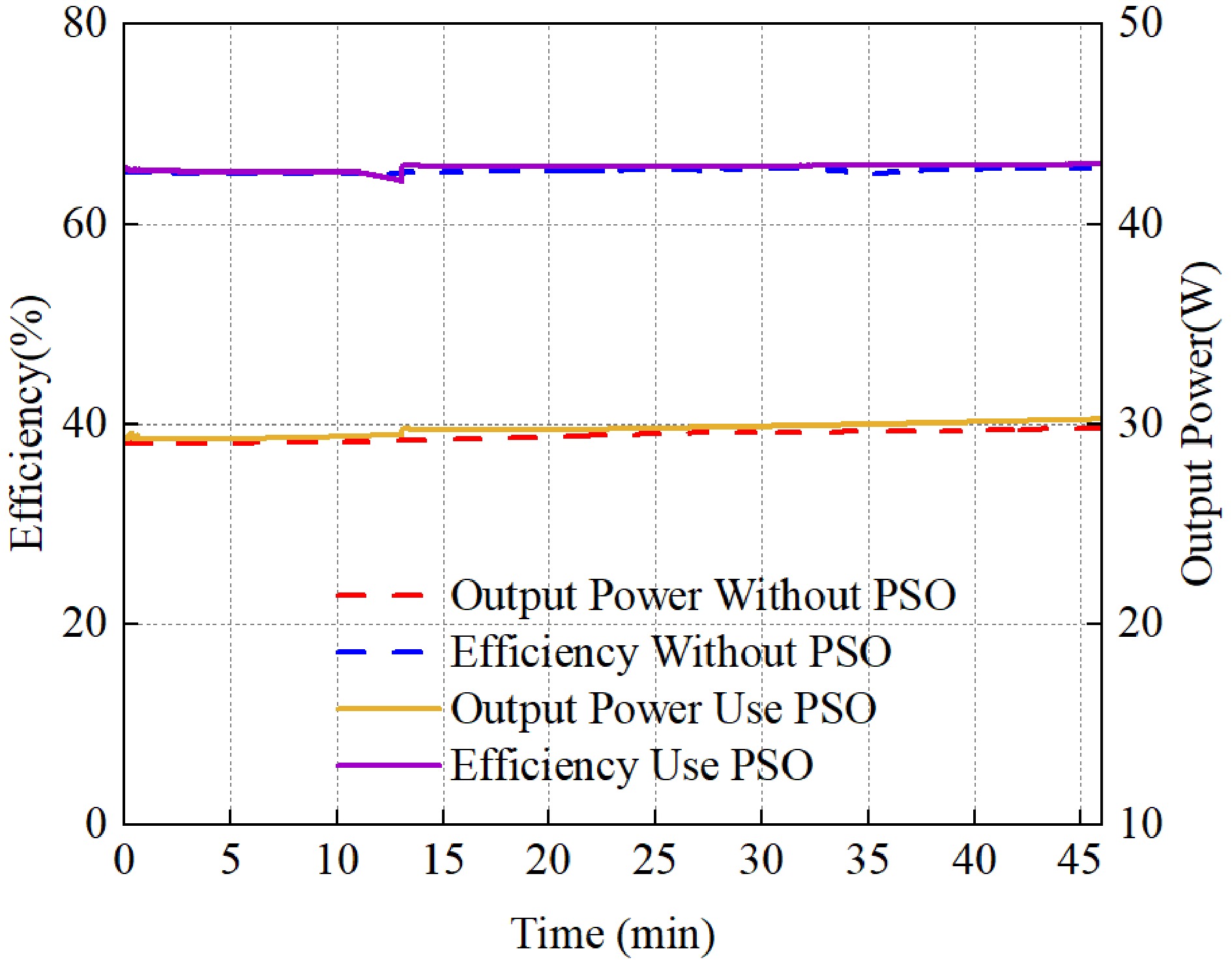
Figure 19.
Charging power and efficiency diagram of the receiving coil at the center of the coil array.
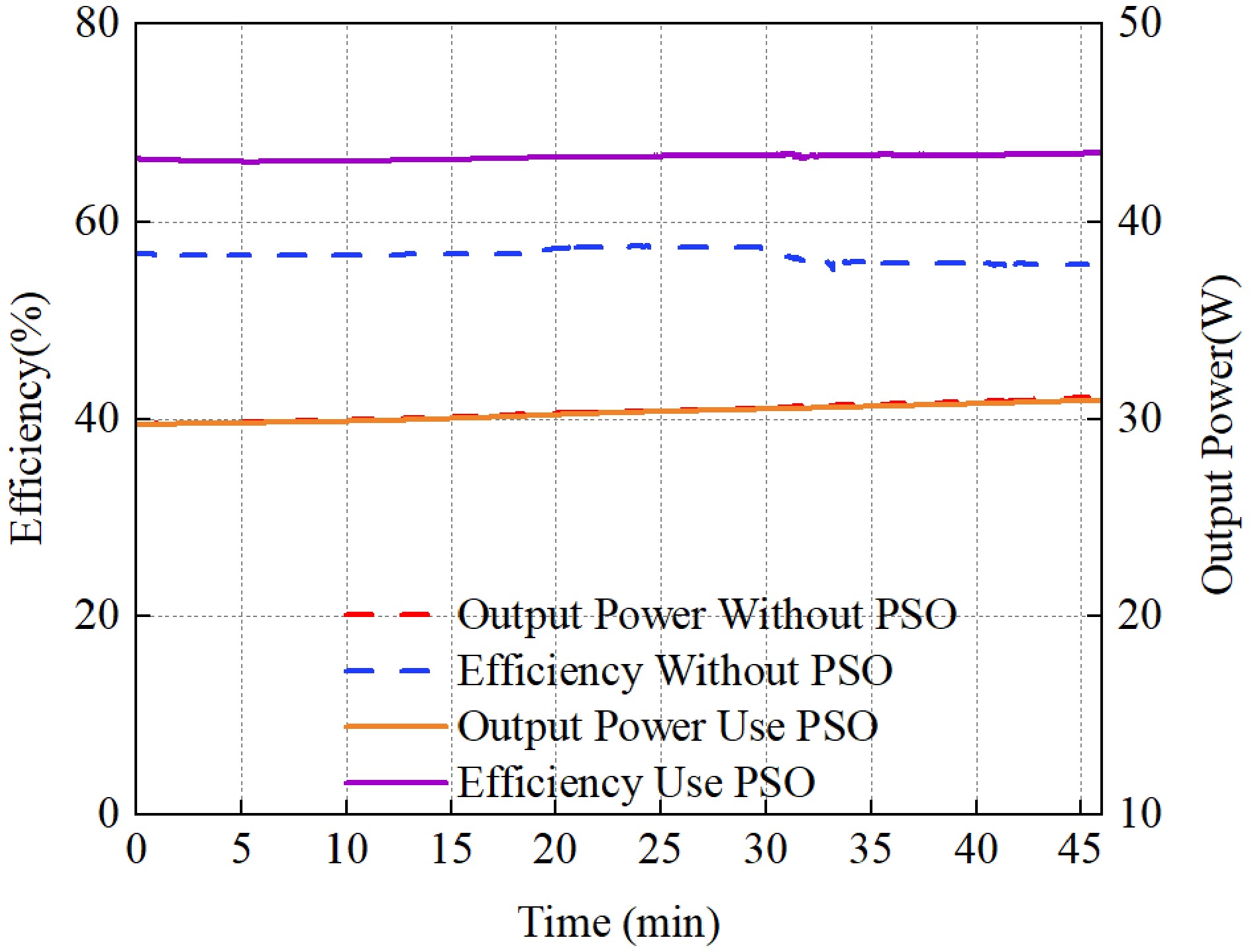
Figure 20.
Charging power and efficiency graph with the transverse offset of the receiving coil by 5 cm.
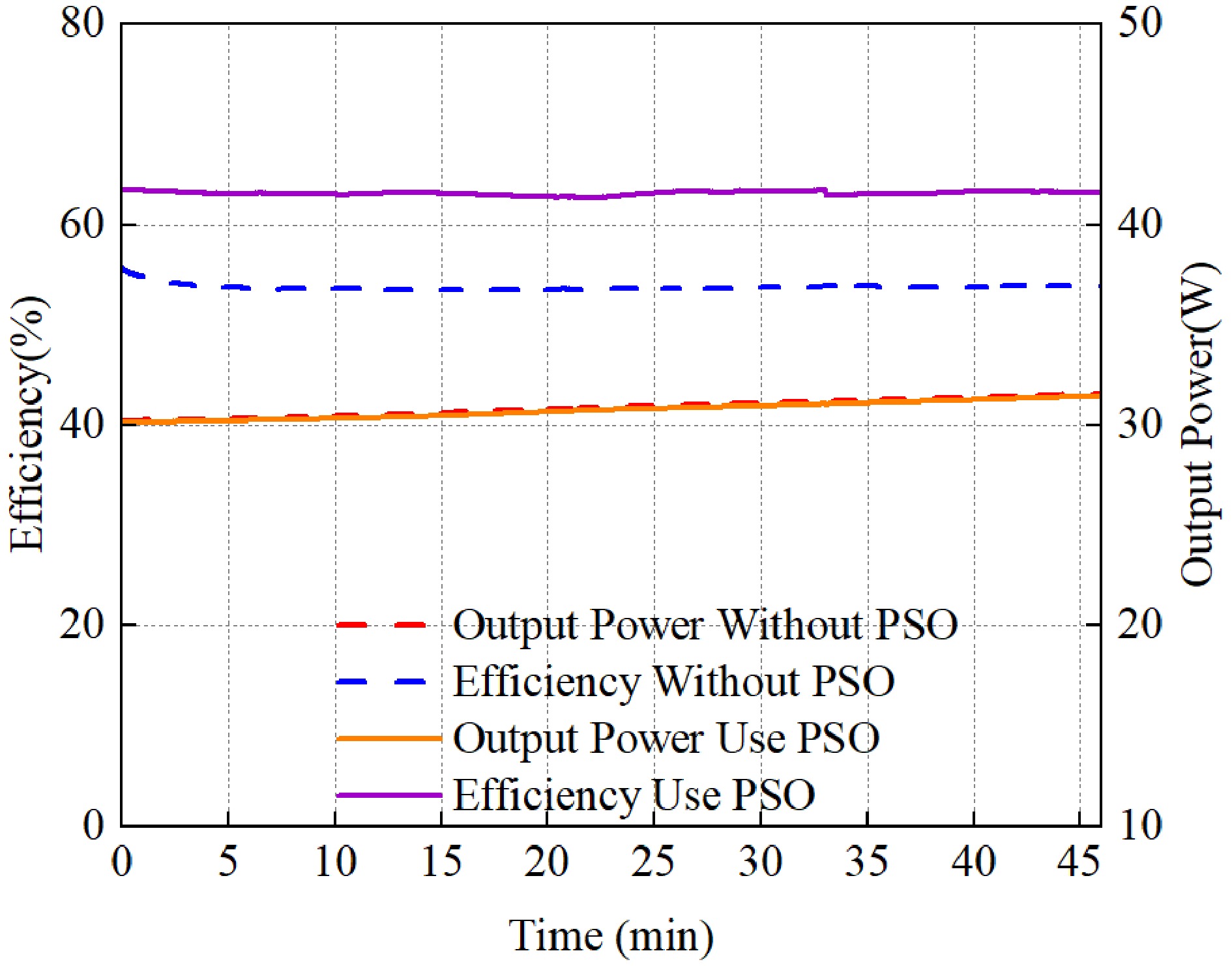
Figure 21.
Graph showing the charging power and efficiency when the diagonal offset of the receiving coil is 5 cm.
Further discussion and prospects
-
To determine the position information of the UAV, the following scheme can be applied to the MTA-WPT system. Based on the different positions of the receiving coil, the phase of the input current
$ {I}_{pn1} $ $ {I}_{pn1} $ $ Ui{n}_{n} $ $ {I}_{pn1} $ $ Ui{n}_{n} $ $ {I}_{pn1} $ $ Ui{n}_{n} $ -
This study investigates the charging efficiency and power output of a UAV landing at different positions within a multi-transmitter coil array. Experimental results demonstrate that the amplitude and phase allocation strategy optimized by the proposed Particle Swarm Optimization (PSO) algorithm can effectively improve the system efficiency under UAV landing misalignment conditions. Specifically, with a 20
$ \Omega $ -
The authors confirm their contributions to the paper as follows: study conception and design: Zhang Y, Liu Y, Xu J, Pang S; data collection: Liu Y, Li C, Yang S; analysis and interpretation of results: Yang Y, Liu Y, Xu J, Pang S; draft manuscript preparation: Liu Y, Xu J, Pang S, Li H. All authors reviewed the results and approved the final version of the manuscript.
-
The datasets generated during and/or analyzed in the current study are available from the corresponding author upon reasonable request.
-
The authors declare that they have no conflict of interest.
- Copyright: © 2026 by the author(s). Published by Maximum Academic Press, Fayetteville, GA. This article is an open access article distributed under Creative Commons Attribution License (CC BY 4.0), visit https://creativecommons.org/licenses/by/4.0/.
-
About this article
Cite this article
Li H, Liu Y, Pang S, Xu J, Yang Y, et al. 2026. Research on multi-coil wireless charging efficiency optimization system for unmanned aerial vehicles: based on input control and PSO algorithm. Wireless Power Transfer 13: e030 doi: 10.48130/wpt-0026-0018 

Research on multi-coil wireless charging efficiency optimization system for unmanned aerial vehicles: based on input control and PSO algorithm
- Received: 14 January 2026
- Revised: 29 April 2026
- Accepted: 06 May 2026
- Published online: 28 October 2026
Abstract: To address the significant impact of positional deviation during unmanned aerial vehicle (UAV) landing on the power transfer efficiency of wireless power transfer (WPT) systems, this paper proposes a Multi-Transmitter Array Wireless Power Transfer (MTA-WPT) system. A theoretical analysis is conducted on the influence of input voltage amplitude and phase on receiver power and efficiency under different mutual inductance matrices. Through simulation, a topology with five transmitting coils and one receiving coil is ultimately selected. By introducing a Particle Swarm Optimization (PSO) algorithm to adjust the input voltage amplitude and phase, the system achieves improved charging efficiency while maintaining stable power output during the horizontal translation of the receiver above the coil array. Experimental validation demonstrates that when the UAV battery is charged at a power level of approximately 30 W, the system efficiency increases by up to 10.16 % compared to operation without algorithm control. The proposed solution effectively mitigates charging instability caused by inaccurate UAV landing, providing reliable wireless charging support for UAVs under positional offset.