A dynamic interaction assessment method for disaster management based on extended DEMATEL

For the past few years, despite great advances in science and technology, various disasters, such as earthquakes, landslides, hurricanes, industrial explosions and fires, have posed severely negative impacts on human being’s lives, economic development and social stability. After the occurance of such a devastating disaster, how to conduct reasonable evaluations on emergencies and take effective measures to prevent the escalation of the situation and diminish its impacts is of practical significance. Hence, many researchers have put great effort into an important topic for disaster management, which is how to evaluate emergencies rationally and further take response measures effectively.

Many researchers have investigated the above topic from diverse perspectives. For example, Kapucu & Garayev^[1] studied collaborative disaster management decisions to respond to Hurricanes Rita and Katrina. Hämäläinen et al.^[2] presented a multi-attribute risk analysis method for selecting the response strategy to protect populations after nuclear accident simulation. Mendonça et al.^[3] investigated an approach by use of communication and computerization technologies to deal with two important factors of emergency response including response strategy implementation speed and expert knowledge quality upon which the response is relied. Bryson et al.^[4] recommended a mathematical programming model as a decision support tool to assist decision makers (DMs) to reach successful development of a disaster recovery plan. Lin Moe et al.^[5] put forward a balanced scorecard approach which enables a continuous performance assessment in life-cycle phases of natural disaster management projects. Rolland et al.^[6] developed a decision support system using hybrid meta-heuristics for disaster response and recovery. To improve the efficiency of group decision making faced with disasters, Xie et al.^[7] developed an agile-Delphi method based on network technology. Ju & Wang^[8] employed Dempster-Shafer theory and analytic hierarchy process (AHP) to appraise emergency response solutions with incomplete information. Pérez-González et al.^[9] developed a data analytics platform using statistical models to support emergency and security management of accidents. Cao et al.^[10] focused on an integrated emergency response evaluation method by incorporating cellular automata to choose the best evacuation route for toxic gas release accidents. Mashi et al.^[11] conducted an assessment of Nigeria's National Emergency Management Agency Act for ascertaining its effectiveness and efficiency in disaster risk reduction.

The above reviewed literature are mainly concerned with static emergency assessment or decision making in disaster management. However, as is generally known, the development of disaster is a dynamic evolutionary process and usually involves different emergency scenarios. Hence, many researchers have paid close attention to phased assessments in the light of disaster dynamics. Zhao et al.^[12] introduced an evolutionary decision support method based on a case study considering the dynamic and evolutionary characteristics of emergency response. Yang & Xu^[13] developed an engineering model using dynamic games to produce the optimal relief plan for decision making during disaster management. Liu et al.^[14] focused on an emergency response decision making method based on fault tree analysis considering the characteristics of dynamic evolvement process, multiple emergency scenarios and impact of response measures. Through simulating dynamic processing changes via the event-tree method, Shi et al.^[15] constructed a technique plan repository to dispose chemical pollution accidents, then used a group AHP method to evaluate response plans. Liu et al.^[16] proposed a dynamic grey relational analysis method to appraise the treatment technology of chemical contingency spills. In their study, the method was applied to assess emergency arsenic treatment technology under different scenarios with two arsenic levels.

Nevertheless, research considering disaster dynamics do not take the interactions among the activities of disaster management into account. Whereas, disaster management is a systematic work and covers many aspects that usually have positive or negative influences on each other due to the domino effects of disasters, multi-department collaborative rescue and games between emergency response and disaster. In view of this, Helbing & Kühnert^[17] presented a flexible assessment method for interaction networks, which investigated the effects of indirect interactions and feedback loops and allowed assessment of the effect of optimization measures or failures on disaster management. Buzna et al.^[18] provided a model for the dynamic spreading and cascade failures in directed networks, and explored its properties with regard to different disaster network topologies by virtue of simulations. Weng et al.^[19] presented the spreading dynamics of disaster from key out-degree nodes in complex networked systems, and showed some typical disaster spreading characteristics by simulations. Levy & Taji^[20] developed a group decision support approach in order to assist hazard planning and disaster management under uncertainty. Rehman et al.^[21] considered system thinking approaches to identify key stakeholders in analyzing various flood influencing factors for disaster risk reduction.

The above literature are mainly focussed on the traditional methods of system theory or complex network theory considering the causality among influencing factors of disaster management. However, either the complex causal relationships and roles played in disaster management of factors are not fully dissected, or the dynamic evolutions of factors are not simulated, which are both of great significance for disaster management. The Decision-Making Trial and Evaluation Laboratory (DEMATEL) technique initiated by Gabus & Fontela^[22], utilizes matrices and associated mathematical fundamentals to compute the effect and cause on factors of a system. The matrices or diagrams depict a contextual relationship among the factors, where numerical values denote the strength of influences. The DEMATEL method is capable of revealing the complex causal relationships and converting the interrelations into an intelligible structural model. This method has been extensively applied to address a variety of complex problems, which can effectively interpret complex structures and supply viable options for problem-solving^[23]. However, the DEMATEL method can only capture the strength of direct relations among factors and cannot distinguish the kind of influences among factors, namely positive influence or negative influence, which is essential in figuring out how the factor develops or evolves under the effects exerted by other factors. For disaster management, it is obvious that the development of influencing factors or activities is important in coping with the emergencies. Hence, extending the traditional DEMATEL technique to capture both the negative and positive direct relations between factors of disaster management and further analyzing the factors’ evolution according to the interactions among them is the first motivation of this study.

Furthermore, in the real assessment process, because of the fuzziness and uncertainty of assessment objects in complex emergencies, many problems can only be qualitatively evaluated rather than being quantitatively described. Meanwhile, since language terminologies are close to the human cognition process, experts may feel more intuitionistic and comfortable using them to provide assessments rather than numeric values. Therefore, experts usually prefer to employ linguistic terms to offer evaluation information^[24]. Additionally, in preceding linguistic information processing, when linguistic terms are converted into fuzzy numbers, information distortion or loss often took place and the computation results did not match the initial linguistic terms. To address the above limitations, the 2-tuple fuzzy linguistic model was put forward^[25], which can accurately express and process linguistic information. Many studies have incorporated 2-tuple linguistic model into disaster management evaluation issues^[26,27]. Whereas, in the 2-tuple linguistic model, the linguistic term set actually uses a unipolar scale. With this type of scale, the aspects in negativeness and positiveness of preferences can be portrayed and collected. But, the boundary between negative preference and positive preference such as low and high is not clearly defined or very distinct for the reason that the definitions of both membership functions are on the basis of positive partitions of unit interval. Also, it is shown by many psychological evidence that numerous human beings’ evaluation scores locate at a bipolar scale^[28]. So, it will be productive to include the bipolar 2-tuple linguistic model that uses a bipolar scale in disaster management assessment, which is another motivation for the present study.

Accordingly, in this study a dynamic interaction assessment method for disaster management based on extended DEMATEL is proposed, which is under the bipolar 2-tuple linguistic information environment and takes both involved dynamics and interrelations among influencing factors into account.

This section reviews some concepts of bipolar 2-tuple linguistic information and the classical DEMATEL method.

Bipolar 2-tuple linguistic information

Let $ {{S}} = \{ {{{s}}_{{{ - g} \mathord{\left/ {\vphantom {{ - g} 2}} \right. } 2}}},...,{{ }}{s_0},...,{{ }}{s_{{g \mathord{\left/ {\vphantom {g 2}} \right. } 2}}}\} $ be a bipolar linguistic term set (BLTS), the granularity of $ S $ is $ g + 1 $, $ {s_i} $ denotes a possible bipolar linguistic variable. The following properties are required to be satisfied for a BLTS^[25]:

(1) $ {s_i} > {s_j} $, if $ i > j $

(2) $ {\rm{Neg}} ({s_i}) = {s_{ - i}} $

Definition 1^[28]. Let $ {{S}} = \{ {{{s}}_{{{ - g} \mathord{\left/ {\vphantom {{ - g} 2}} \right. } 2}}},...,{{ }}{s_0},...,{{ }}{s_{{g \mathord{\left/ {\vphantom {g 2}} \right. } 2}}}\} $ be a BLTS, $ \beta \in [{{ - g} \mathord{\left/ {\vphantom {{ - g} {2,}}} \right. } {2,}}{g \mathord{\left/ {\vphantom {g 2}} \right. } 2}] $ be an aggregation value of linguistic symbol. The definition of a bipolar 2-tuple is given as:

where the index label of $ {s_i} $ is closest to $ \beta $, $ round( \cdot ) $ is the rounding operation, $ \alpha $ is the symbolic translation value.

Definition 2. Let $ {{S}} = \{ {{{s}}_{{{ - g} \mathord{\left/ {\vphantom {{ - g} 2}} \right. } 2}}},...,{{ }}{s_0},...,{{ }}{s_{{g \mathord{\left/ {\vphantom {g 2}} \right. } 2}}}\} $ be a BLTS, $ ({s_i},\alpha ) $ be a bipolar 2-tuple. A function $ {\Delta ^{ - 1}} $ to transform $ ({s_i},\alpha ) $ into its equivalent value $ \beta \in [{{ - g} \mathord{\left/ {\vphantom {{ - g} {2,}}} \right. } {2,}}{g \mathord{\left/ {\vphantom {g 2}} \right. } 2}] $ is defined as:

Obviously, a bipolar 2-tuple $ ({s_i},0) $ can be transformed from a linguistic term $ {s_i} $.

Theorem 1. The comparison of any two bipolar 2-tuples $ ({s_m},{\alpha _m}) $ and $ ({s_n},{\alpha _n}) $ is conducted in term of an ordinary lexicographic order:

(1) $ ({{{s}}_{{m}}},{\alpha _m}) < ({{{s}}_{{n}}},{\alpha _n}) $, if $ m < n $;

(2) $ ({{{s}}_{{m}}},{\alpha _m}) < ({{{s}}_{{n}}},{\alpha _n}) $, if $ m = n $ and $ {\alpha _m} < {\alpha _n} $;

(3) $ ({{{s}}_{{m}}},{\alpha _m}) > ({{{s}}_{{n}}},{\alpha _n}) $, if $ m = n $ and $ {\alpha _m} > {\alpha _n} $.

Definition 3. Let $ X = \{ ({{{s}}_1},{\alpha _1}),({{{s}}_2},{\alpha _2}),...,({{{s}}_n},{\alpha _n})\} $ be a bipolar 2-tuple set, its associated weight vector be $ w = {({w_1},{w_2},...,{w_n})^T} $, $ 0 \leqslant {w_i} \leqslant 1 $ and $ \displaystyle\sum\limits_{i = 1}^n {{w_i}} = 1 $. The definition of bipolar 2-tuple weighted average (BTWA) operator is given as:

The DEMATEL method

The steps of classical DEMATEL are outlined below^[23].

Step 1: Determine the decision object and its influential factors $ F = \left\{ {{{{F}}_1},{{{F}}_2},...,{{{F}}_{{n}}}} \right\} $.

Step 2: Establish an expert group, denoted as $ E = \left\{ {{E_1},{E_2},...,{E_K}} \right\} $, and invite the experts to appraise the direct influence between each factor pair, adopting the integer scale: '0-no influence', '1-low influence', '2-medium influence', '3-high influence' and '4-very high influence'. Experts' assessments are arranged in individual direct relation matrices $ {X_k} = {[x_{ij}^k]_{n \times n}}(k = 1,2,...,K) $, where $ x_{ij}^k{{ }}(i,j = 1,2,...,n) $ indicates the degree of $ {F_i} $ influencing $ {F_j} $ and $ x_{ii}^k $ are set as 0. The direct relation matrice $ X = {[{x_{ij}}]_{n \times n}} $ is acquired through aggregating individual assessment matrices, where:

Step 3: Normalize the direct relation matrice $ X = {[{x_{ij}}]_{n \times n}} $ as $ D = {[{d_{ij}}]_{n \times n}} $ by Eqs. (5) − (6), where $ 0 \leqslant {d_{ij}} < 1 $.

Step 4: Generate the total relation matrice $ T $through summing both direct influences and indirect influences among factors, i.e.,

where E is an $ n \times n $ identity matrice.

Step 5: Compute the row sum R and column sum C of T as:

where $ {r_i} $ denotes the total influences exerting to others of factor $ {F_i} $, $ {c_j} $ denotes the total influences received from others of factor $ {F_j} $.

Step 6: Construct the causal diagram by placing the prominence and relation values ($ R + C $ and $ R - C $) on the horizontal and vertical axes, respectively. Here, the factor importance is shown by the horizontal axis, factors are divided by the vertical axis into effect group with $ {r_i} - {c_i} < 0 $ of a factor and cause group with $ {r_i} - {c_i} > 0 $ of a factor.

In this section, a dynamic interaction assessment method for disaster management based on the extended DEMATEL with bipolar 2-tuple linguistic information is proposed. Figure 1 displays its flowchart.

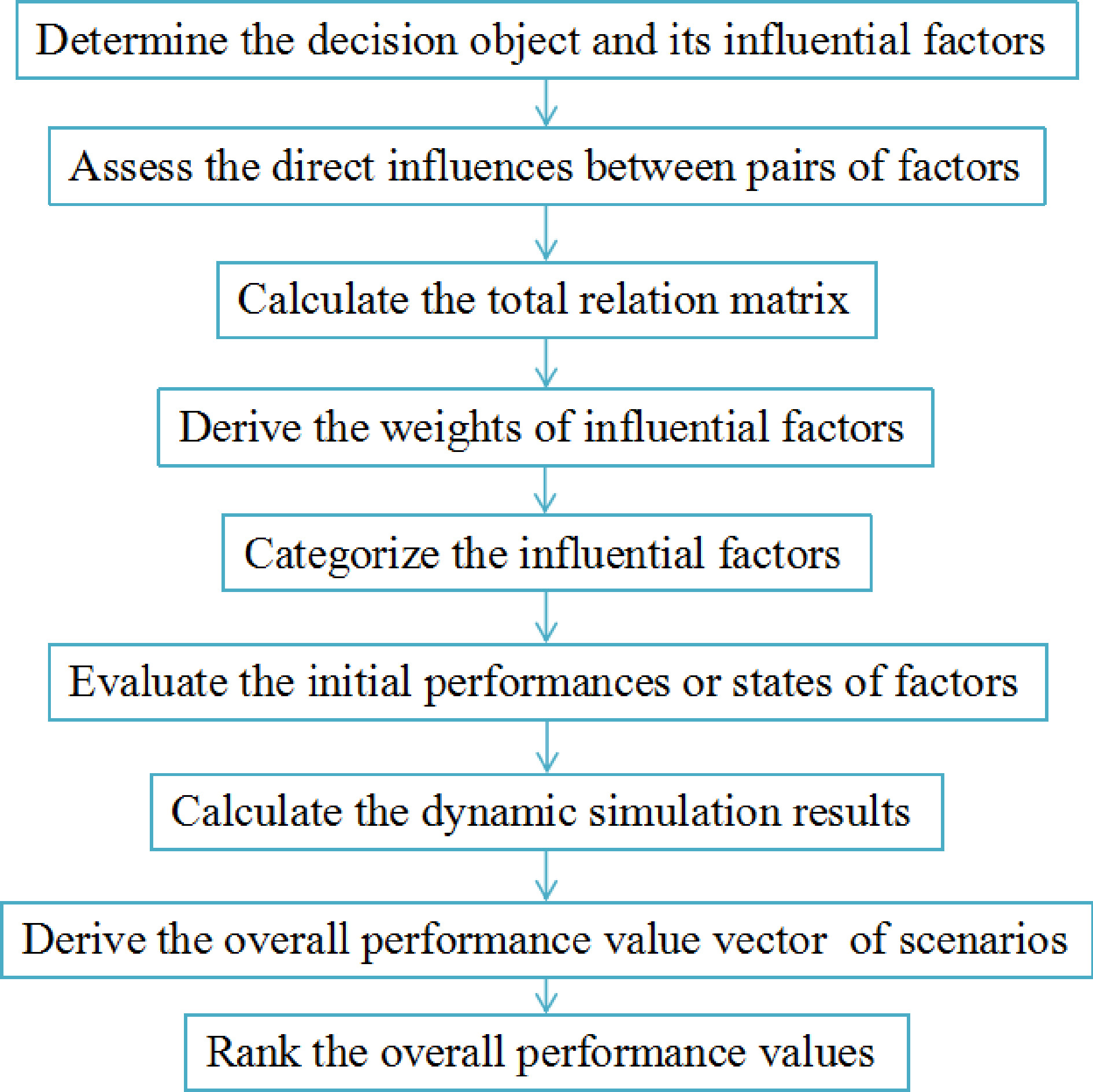
Figure 1. 

Flowchart of the suggested method.

Let $ E = \left\{ {{E_1},{E_2},...,{E_K}} \right\} $ be an invited expert panel with relevant backgrounds and knowledge about disaster management, and $ t = \left\{ {{{{t}}_1},{{{t}}_2},...,{{{t}}_{{P}}}} \right\} $ be the set of time points at which DMs decide to assess possible emergency scenarios and make decisions to deal with the disaster. Suppose $ {\hat E^{{{{t}}_p}}} = \left\{ {{{\hat e}}_1^{{{{t}}_p}},{{\hat e}}_2^{{{{t}}_p}},...,{{\hat e}}_{{Q}}^{{{{t}}_p}}} \right\} $ be the set of possible emergency scenarios at time point $ {{{t}}_p}(p = 1,2,...,P) $, then the evaluation process of one of the emergency scenarios at a certain time point such as $ {{\hat e}}_q^{{{{t}}_p}}(q = 1,2,...,Q) $ is proposed as follows.

Step 1: Determine the emergency scenario $ {{\hat e}}_q^{{{{t}}_p}} $ during disaster management as decision object, and its influential factors $ F = \left\{ {{{{F}}_1},{{{F}}_2},...,{{{F}}_{{n}}}} \right\} $ can be decided by the expert group from aspects such as the destructiveness of disaster, disaster-affected bodies, disaster prevention and control measures, and uncontrolled nature forces.

Step 2: Invite the expert group to assess the direct influences within factor pairs using the linguistic term set such as S = {s_-4 = very high negative influence, s_-3 = high negative influence, s_-2 = medium negative influence, s_-1 = low negative influence, s₀ = no influence, s₁ = low positive influence, s₂ = medium positive influence, s₃ = high positive influence, s₄ = very high positive influence}, and then denote the individual fuzzy linguistic direct relation matrices furnished by experts as $ {\bar A_k} = {[a_{ij}^k]_{n \times n}}(k = 1,2,...,K) $, where $ a_{ij}^k $ represents linguistic evaluation on the influence degree of $ {F_i} $ on $ {F_j} $ given by expert $ {E_k} $ and elements of main diagonal $ a_{ii}^k $ are set to s₀.

Step 3: Transform $ {\bar A_k} = {[a_{ij}^k]_{n \times n}} $ into bipolar 2-tuple linguistic direct relation matrices (BTLDRMs) $ {A_k} = {[(a_{ij}^k,0)]_{n \times n}} $.

Step 4: Produce the collective BTLDRM $ A = {[({a_{ij}},{\alpha _{ij}})]_{n \times n}} $ through aggregating the individual BTLDRMs, where:

Step 5: Sum direct influences and indirect influences produced by feedback loops to derive the total relation matrice $ \bar T $ as follows:

To ensure Eq. (11) converge, the following formula is suggested instead^[17]:

where $ {e^A} $ is the exponential of matrice $ A $, $ E $ is an $ n \times n $ identity matrice, $ \hat t $ can be regarded as the virtual time step indicating the influences over $ \hat t - 1 $ factor(s) during this period of time, i.e. $ \hat t = 1 $ indicates direct influences, $ \hat t = 2 $ indicates feedback loops with one intermediate factor, etc. Besides, note that the elements of $ A $ that are in the form of bipolar 2-tuples shall be transformed into their equivalent values according to Definition 2 during calculation.

Step 6: Compute the row sum $ \bar R $ and column sum $ \bar C $ of $ \bar T $.

Step 7: Derive the weight vector $ {{{w}}^{{{\hat e}}_q^{{{{t}}_p}}}} = [w_1^{{{\hat e}}_q^{{{{t}}_p}}},w_2^{{{\hat e}}_q^{{{{t}}_p}}},...,w_n^{{{\hat e}}_q^{{{{t}}_p}}}] $ of influential factors involved in scenario $ {{\hat e}}_q^{{{{t}}_p}} $ in term of their prominence $ \bar R + \bar C $ and relation $ \bar R - \bar C $.

Step 8: Construct the causal diagram and categorize the influential factors into effect group and cause group.

Step 9: Evaluate the initial performance or state of each factor without being affected by other factors due to the interactions among them, then denote the assessments as $ {{{\bar R}}^k} = [{{r}}_1^k,{{r}}_2^k,...,{{r}}_{{n}}^k] $, where $ {{r}}_i^k(i = 1,2,...,n) $ represent the fuzzy linguistic assessment on the initial performance or state of factor $ {F_i} $ supplied by expert $ {E_k} $ employing the predefined linguistic term sets.

Step 10: Transform the fuzzy linguistic assessments $ {{{\bar R}}^k} = [{{r}}_1^k,{{r}}_2^k,...,{{r}}_{{n}}^k] $ into bipolar 2-tuple linguistic assessments (BTLAs) $ {{{R}}^k} = [({{r}}_1^k,0),({{r}}_2^k,0),...,({{r}}_{{n}}^k,0)] $.

Step 11: Aggregate the individual assessments to obtain the collective BTLAs $ {{R}} = [({{{r}}_1},{\varepsilon _1}),({{{r}}_2},{\varepsilon _2}),...,({{{r}}_n},{\varepsilon _n})] $, where:

Step 12: Calculate the dynamic simulation performance or state values of factors.

At each virtual time step $ {t_v}({t_v} \geqslant 1) $, the dynamic simulation performance or state values $ {{{R}}^{{t_v}}} = [\xi _1^{{t_v}},\xi _2^{{t_v}},...,\xi _n^{{t_v}}] $ of factors are computed by adding the changes caused by the influences of other factors to their initial performance or states according to the following rule:

where the elements of R and A expressed by bipolar 2-tuples shall be converted into their equivalent values in calculation according to Definition 2.

Based on Eq.(12), if $ {t_v} \to \infty $, then $ {{{R}}^{{t_v}}} = {{R}} + {{R}}({e^A} - E) $, which is the stable state for factors. Here, for fast convergence, it is considered at the stable states when any element $ {\chi _{ij}} $ in $ \displaystyle\sum\limits_{\hat t = 1}^{{t_v}} {\frac{{{A^{\hat t}}}}{{\hat t!}}} $ and $ {\eta _{ij}} $ in $ ({e^A} - E) $ meet $ \left| {{\chi _{ij}} - {\eta _{ij}}} \right| < 0.0001 $, then denote the stable state values of factors involved in current emergency scenario $ {{\hat e}}_q^{{{{t}}_p}} $ as $ {{{R}}^{{{\hat e}}_q^{{{{t}}_p}}}} = [\xi _1^{{{\hat e}}_q^{{{{t}}_p}}},\xi _2^{{{\hat e}}_q^{{{{t}}_p}}},...,\xi _n^{{{\hat e}}_q^{{{{t}}_p}}}] $.

Step 13: The weight vectors and stable state values of factors in other emergency scenarios in set $ {\hat E^{{{{t}}_p}}} = \left\{ {{{\hat e}}_1^{{{{t}}_p}},{{\hat e}}_2^{{{{t}}_p}},...,{{\hat e}}_{{Q}}^{{{{t}}_p}}} \right\} $ at time point $ {{{t}}_p} $ can also be obtained through the above evaluation process. Then, put the weight vectors and stable state values of factors in all scenarios at time point $ {{{t}}_p} $ into the matrice $ {{{W}}^{{t_p}}} = {[w_{ij}^{{t_p}}]_{Q \times {n_{dif f}}}}\; $ and $ {{{R}}^{{t_p}}} = {[r_{ij}^{{t_p}}]_{Q \times {n_{dif f}}}}\; $ as below, respectively,

where $ {n_{dif f}} $ is the number of all the different influential factors involved in all emergency scenarios, and for each emergency scenario, the position of factor that is not involved compared with other scenarios shall be filled with 0 in both $ {{{W}}^{{t_p}}} = {[w_{ij}^{{t_p}}]_{Q \times {n_{dif f}}}} \;$ and $ {{{R}}^{{t_p}}} = {[r_{ij}^{{t_p}}]_{Q \times {n_{dif f}}}} $ .

Step 14: Normalize $ {{{R}}^{{t_p}}} = {[r_{ij}^{{t_p}}]_{Q \times {n_{dif f}}}} \;$ into a comparable scale $ {{{\hat R}}^{{t_p}}} = {[\hat r_{ij}^{{t_p}}]_{Q \times {n_{dif f}}}}\; $ to ensure the compatibility among different emergency scenarios:

For benefit factors (B), the bigger their performance or state values, the more advantageous to disaster management, then:

For cost factors (C), the smaller their performance or state values, the more advantageous to disaster management, then:

Step 15: Compute the overall performance value vector $ {V^{{{{t}}_p}}} = [V_1^{{{{t}}_p}},V_2^{{{{t}}_p}},...,V_Q^{{{{t}}_p}}] $ of all emergency scenarios at time point $ {{{t}}_p} $ by weighted average operator, where:

Step 16: Rank the overall performance values of all emergency scenarios at $ {{{t}}_p} $ according to the value of $ V_{{q}}^{{{{t}}_p}} $, based on which DMs can make a decision to deal with the disaster.

By the time point $ {{{t}}_{p + 1}} $, if the disaster is not controlled and further prevention and control measures need to be taken, DMs may decide to implement the evaluation of possible emergency scenarios at time point $ {{{t}}_{p + 1}} $, then the evaluation process can be carried out at the time point $ {{{t}}_p} $.

An example is displayed in this section to illustrate the application and feasibility of the recommended dynamic interaction assessment method for disaster management.

On 4 October 2015, in Zhanjiang (Guangdong, China), affected by 'Typhoon Mujigae', three tanks containing more than 800 tons of liquefied petroleum gas leaked simultaneously and explosion could occur at any time. Tank No. 1 were leaking both top and bottom, tanks No. 2 and 3 were leaking on the bottom. Considering the good natural dilution conditions with strong winds and rain from time to time and adequate preparation for manual air dilution in the leaking area, provincial and municipal experts thought the interaction or interdependency existing among the three leaked tanks was almost negligible and controllable, and determined the best rescue plan as: protecting tank No. 1; plugging the leaking holes of tanks No. 2 and 3 after the completion of the natural leakage of tank No. 1, and finally transporting and reverse irrigation for residual gas in tanks No. 2 and 3^[29] (https://www.sohu.com/a/39229303_120002). Here, to demonstrate the application of the method in a typical emergency scenario, the illustrative example is adapted from the above case with only one leaking liquefied petroleum gas tank (No. 3) being considered. Two different time points $ t = \left\{ {{{{t}}_1},{{{t}}_2}} \right\} $ at which evaluations are initiated according to the real situation of disaster management are determined and three invited experts participate in evaluation. Also, to save space, influencing factors of emergency scenarios at $ {{{t}}_1} $ and $ {{{t}}_2} $ that are identified by expert analysis based on the real situation of disaster management are presented together in Table 1.

(1) Assessment at time point t₁

At $ {{{t}}_1} $, emergency management departments receive the alarm and organize disaster relief teams to travel to the leakage site for rescue and evacuation. Due to the effect of typhoon, the main roads to the leakage site are blocked, which delay the search and rescue. But, if traffic departments decide to clear roadblocks and evacuate traffic, more people will seriously suffer from typhoon. So, suppose DMs decide to evaluate two emergency scenarios, in the first one, disaster relief teams clear roadblocks when travelling to the site, and in the second, the traffic department is involved in clearing roadblocks and evacuating traffic. The influential factors for the first emergency scenario $ {{\hat e}}_1^{{{{t}}_1}} $ are identified as $ \left\{ {{{{F}}_1},{{{F}}_2},...,{{{F}}_{10}}} \right\} $ and these of the second emergency scenario $ {{\hat e}}_2^{{{{t}}_1}} $ are $ \left\{ {{{{F}}_1},{{{F}}_2},...,{{{F}}_{11}}} \right\} $ as shown in Table 1.

For scenarios $ {{\hat e}}_1^{{{{t}}_1}} $ and $ {{\hat e}}_2^{{{{t}}_1}} $, experts provide their judgments about the direct influences between each pair of factors employing the linguistic term set S given in Step 2 of the proposed method, about which the collective BTLDRM $ {A_{{t_1}}} $ is shown in Table 2. The initial performances or states of factors are also evaluated by experts using the linguistic term sets S_a, S_b and S_c, of which the collective BTLAs $ {{{R}}_{{t_1}}} $ are given in Table 2. Specifically, the initial performances or states of $ \left\{ {{{{F}}_1}} \right\} $, $ \left\{ {{{{F}}_2},{{{F}}_3},{{{F}}_4},{{{F}}_5},{{{F}}_6}} \right\} $ and $ \left\{ {{{{F}}_7},{{{F}}_8},{{{F}}_9},{{{F}}_{10}},{{{F}}_{11}}} \right\} $ are assessed according to S_a, S_b and S_c for experts intuitively and comfortably expressing their assessments, respectively. Note that considering the commonness between $ {{\hat e}}_1^{{{{t}}_1}} $ and $ {{\hat e}}_2^{{{{t}}_1}} $, the assessments in Table 2 on the first 10 factors of $ {{\hat e}}_1^{{{{t}}_1}} $ and $ {{\hat e}}_2^{{{{t}}_1}} $ are the same.

The weight vectors of influential factors of emergency scenarios $ {{\hat e}}_1^{{{{t}}_1}} $ and $ {{\hat e}}_2^{{{{t}}_1}} $ are derived as $ {{{w}}^{{{\hat e}}_1^{{{{t}}_1}}}} $ = [0.08, 0.007, 0.068, 0.117, 0.093, 0.159, 0.042, 0.114, 0.192, 0.127] and $ {{{w}}^{{{\hat e}}_2^{{{{t}}_1}}}} $ = [0.115, 0.005, 0.059, 0.098, 0.089, 0.144, 0.032, 0.087, 0.164, 0.115, 0.093], respectively. It can be found that $ {{{F}}_6} $, $ {{{F}}_9} $, and $ {{{F}}_{10}} $ are the top three critical factors for both scenarios, which is in line with the main object of time point $ {{{t}}_1} $: rescue and evacuation. The weight of $ {{{F}}_1} $ of $ {{\hat e}}_2^{{{{t}}_1}} $ is also in the top three, this is because the typhoon has non-negligible effects on $ {{{F}}_{11}} $ by which other critical factors such as $ {{{F}}_6} $, $ {{{F}}_9} $ and $ {{{F}}_{10}} $ are influenced in comparison with $ {{\hat e}}_1^{{{{t}}_1}} $. The causal diagrams of factors of both emergency scenarios are shown in Fig. 2. Based on Fig. 2, it can be seen that $ {{{F}}_5} $, $ {{{F}}_6} $ and $ {{{F}}_{10}} $ of $ {{\hat e}}_1^{{{{t}}_1}} $ are effect factors, which indicates these factors receive more influence than these exerting on other factors, and others are cause factors. For $ {{\hat e}}_2^{{{{t}}_1}} $, except $ {{{F}}_5} $, $ {{{F}}_6} $ and $ {{{F}}_{10}} $, $ {{{F}}_3} $, $ {{{F}}_4} $ and $ {{{F}}_9} $ with little net effects are also classified into the effect group because of the additional influences received from $ {{{F}}_{11}} $ directly or indirectly.

Figure 2. 

Causal diagrams of factors of emergency scenarios $ {{\hat e}}_1^{{{{t}}_1}} $ and $ {{\hat e}}_2^{{{{t}}_1}} $. (a) for $ {{\hat e}}_1^{{{{t}}_1}} $; (b) for $ {{\hat e}}_2^{{{{t}}_1}} $.

The dynamic simulation performance or state values of factors of scenarios $ {{\hat e}}_1^{{{{t}}_1}} $ and $ {{\hat e}}_2^{{{{t}}_1}} $ are vividly shown in Fig. 3, evolutions of which end after 14 virtual time steps. It can be found that though $ {{{F}}_{11}} $ is negatively affected by the typhoon, the developments of other factors except $ {{{F}}_1} $ and $ {{{F}}_2} $ are promoted towards the states benefiting disaster management due to the total influences of $ {{{F}}_{11}} $, especially $ {{{F}}_5} $, $ {{{F}}_6} $, $ {{{F}}_9} $ and $ {{{F}}_{10}} $, which agrees with the real situation. Further, the overall performance values of two emergency scenarios are derived as 0 and 0.788, which shows that the introduction of clearing roadblocks and evacuating traffic by the traffic department in $ {{\hat e}}_2^{{{{t}}_1}} $ leads the factors to different stable states from these in $ {{\hat e}}_1^{{{{t}}_1}} $ and contributes positively to the current disaster management.

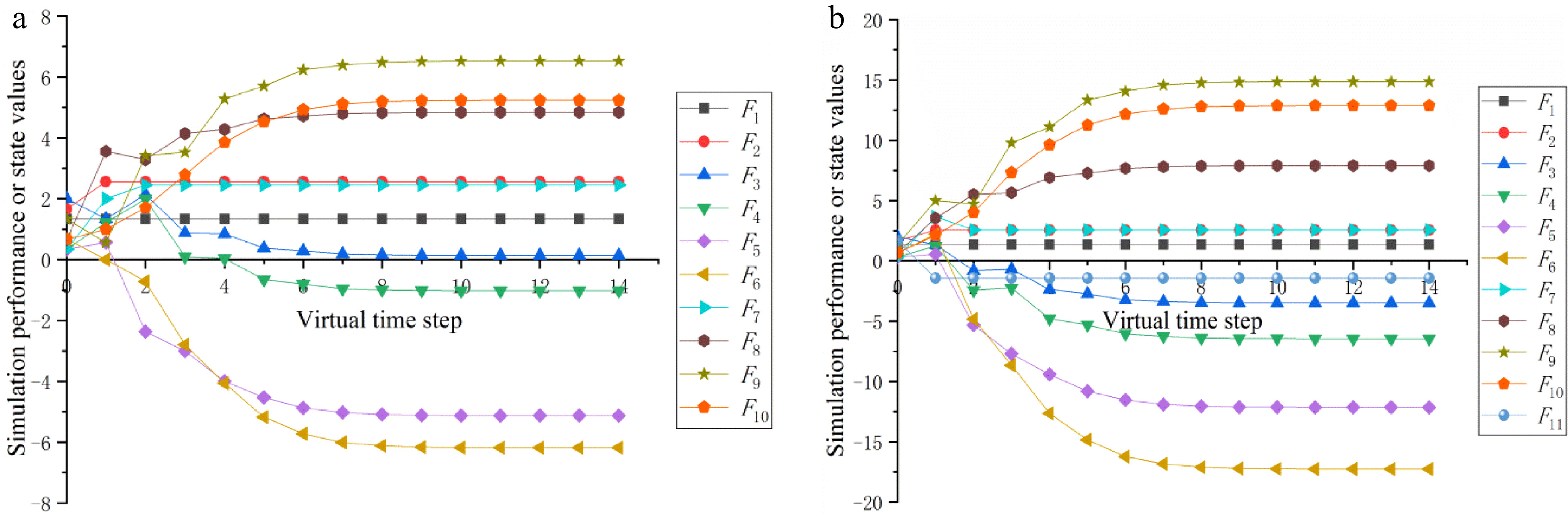
Figure 3. 

Evolutions of simulation performance or state values of factors of emergency scenarios $ {{\hat e}}_1^{{{{t}}_1}} $ and $ {{\hat e}}_2^{{{{t}}_1}} $. (a) for $ {{\hat e}}_1^{{{{t}}_1}} $; (b) for $ {{\hat e}}_2^{{{{t}}_1}} $.

(2) Assessment at time point t₂

At $ {{{t}}_2} $, the typhoon weakens. DMs decide to implement the leakage stoppage and then shift the remaining liquefied petroleum gas to a safe place under the protection of manually diluting the air in the leaking area. But, an appropriate occasion is critical to the success of leakage stoppage that mainly depends on the pressure inside the tank. So, when to stop releasing gas pressure with the leaking hole without human intervention ($ {{{F}}_7} $) needs a decision through assessment. If too early, the high pressure inside the tank will go against the leakage plugging, causing an even greater danger. If too late, too much gas will be released and pose a larger burden to rescue and manual dilution. Here, in order to figure out how $ {{{F}}_7} $ and its interactions with other factors affect the disaster management, suppose there are three emergency scenarios $ \left\{ {{{\hat e}}_1^{{{{t}}_2}},{{\hat e}}_2^{{{{t}}_2}},{{\hat e}}_3^{{{{t}}_2}}} \right\} $ corresponding to three different states of $ {{{F}}_7} $. The above three different states are predefined as follows: if the pressure inside the tank is between 4 and 5 MPa, the state of $ {{{F}}_7} $ is considered as 'very good' that is the first state; if higher than 5 MPa, the state of $ {{{F}}_7} $ is predefined as 'poor', which is the second state; if lower than 4 MPa, the third state of $ {{{F}}_7} $ is regarded as 'medium'. The influential factors involved at $ {{{t}}_2} $ are identified as $ \left\{ {{{{F}}_1},{{{F}}_2},{{{F}}_3},{{{F}}_5},{{{F}}_6},{{{F}}_7},{{{F}}_9},{{{F}}_{12}},{{{F}}_{13}},{{{F}}_{14}}} \right\} $ given in Table 1. Additionally, the initial performances or states of $ \left\{ {{{{F}}_1}} \right\} $, $ \left\{ {{{{F}}_2},{{{F}}_3},{{{F}}_5},{{{F}}_6}} \right\} $ and $ \left\{ {{{{F}}_7},{{{F}}_9},{{{F}}_{12}},{{{F}}_{13}},{{{F}}_{14}}} \right\} $ are appraised according to S_a, S_b and S_c as employed at $ {{{t}}_1} $, respectively.

For scenario $ {{\hat e}}_1^{{{{t}}_2}} $, the collective BTLDRM $ {A_{{t_2}}} $ given by experts is presented in Table 3. For $ {{\hat e}}_2^{{{{t}}_2}} $ and $ {{\hat e}}_3^{{{{t}}_2}} $, assessments on the direct relations between factors are the same as those of $ {{\hat e}}_1^{{{{t}}_2}} $, except the evaluations about the influence degrees of factor $ {F_7} $ on others, which are {(s₀,0), (s₀,0), (s₀,0), (s₀,0), (s₀,0), (s₀,0), (s₁,−0.333), (s₁,0), (s_-2,0.333), (s₀,0)} for $ {{\hat e}}_2^{{{{t}}_2}} $ and {(s₀,0), (s₀,0), (s₀,0), (s₀,0), (s₀,0), (s₀,0), (s₁,0), (s_-1,0.333), (s₂,−0.333), (s₀,0)} for $ {{\hat e}}_3^{{{{t}}_2}} $. The initial performances of $ {F_7} $ in $ {{\hat e}}_1^{{{{t}}_2}} $, $ {{\hat e}}_2^{{{{t}}_2}} $ and $ {{\hat e}}_3^{{{{t}}_2}} $ are predefined as (s₂,0), (s_-1,0) and (s₀,0), respectively. And other factors’ initial performances or states are evaluated as {(s_-2,0.333), (s₁,0.333), (s₂,−0.333), (s₀,−0.333), (s_-1,−0.333), (s₂,0), (s₁,0.333), (s₂,−0.333), (s₂,−0.333) , (s₂,−0.333)} for all three scenarios.

The weight vectors of influential factors of emergency scenarios $ {{\hat e}}_1^{{{{t}}_2}} $, $ {{\hat e}}_2^{{{{t}}_2}} $ and $ {{\hat e}}_3^{{{{t}}_2}} $ are derived as $ {{{w}}^{{{\hat e}}_1^{{{{t}}_2}}}} $ = [0.007, 0.027, 0.149, 0.138, 0.056, 0.139, 0.181, 0.086, 0.129, 0.088], $ {{{w}}^{{{\hat e}}_2^{{{{t}}_2}}}} $ = [0.006, 0.075, 0.158, 0.145, 0.060, 0.019, 0.196, 0.104, 0.145, 0.092] and $ {{{w}}^{{{\hat e}}_3^{{{{t}}_2}}}} $ = [0.006, 0.048, 0.155, 0.142, 0.057, 0.080, 0.192, 0.092, 0.137, 0.092], respectively. It can be found that $ {F_3} $, $ {F_5} $, $ {F_9} $ and $ {F_{13}} $ have greater importance for all emergency scenarios, which is in line with the fact that rescue and leakage stoppage are the core missions of disaster management targeted at addressing the leakage and diminishing the potential explosion risk at time point $ {{{t}}_2} $. Since the people at risk substantially reduce after evacuation at $ {{{t}}_1} $, it is reasonable that the weight of $ {F_6} $ gets smaller. Besides, the role of $ {F_7} $ played in $ {{\hat e}}_1^{{{{t}}_2}} $ is obviously more important than those in $ {{\hat e}}_2^{{{{t}}_2}} $ and $ {{\hat e}}_3^{{{{t}}_2}} $ for the reason that the state of $ {F_7} $ and its influences exerted to other factors in $ {{\hat e}}_1^{{{{t}}_2}} $ are more helpful for disaster management. Figure 4 presents the causal diagrams of factors, from which it can been seen that $ {{{F}}_1} $, $ {{{F}}_2} $, $ {{{F}}_7} $, $ {{{F}}_9} $, $ {{{F}}_{12}} $ and $ {{{F}}_{13}} $ are cause factors and others are effect factors for all three scenarios. Different states of $ {F_7} $ have different direct relations with other factors and further produce different interrelationships among factors as shown in Fig. 4.

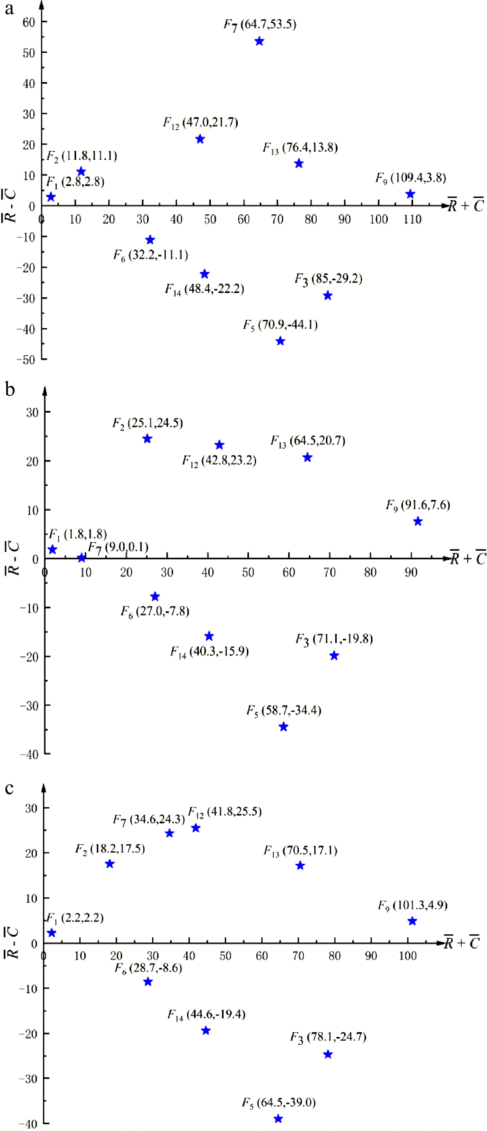
Figure 4. 

Causal diagrams of factors of emergency scenarios $ {{\hat e}}_1^{{{{t}}_2}} $, $ {{\hat e}}_2^{{{{t}}_2}} $ and $ {{\hat e}}_3^{{{{t}}_2}} $. (a) for $ {{\hat e}}_1^{{{{t}}_2}} $; (b) for $ {{\hat e}}_2^{{{{t}}_2}} $; (c) for $ {{\hat e}}_3^{{{{t}}_2}} $.

The dynamic simulation performance or state values of factors of scenarios $ {{\hat e}}_1^{{{{t}}_2}} $, $ {{\hat e}}_2^{{{{t}}_2}} $ and $ {{\hat e}}_3^{{{{t}}_2}} $ are displayed in Fig. 5. The stable states for factors are reached after 14 virtual time steps. Apparently, the different states of $ {F_7} $ and its influences exerted to others bring about different stable states of factors. The overall performance values of three scenarios are obtained as 0.966, 0.008 and 0.007, which suggests that the first state of $ {F_7} $, namely the pressure inside the tank between 4MPa and 5MPa, is more beneficial to disaster management than other states as approved by experts and agreeing with the aforementioned assumption.

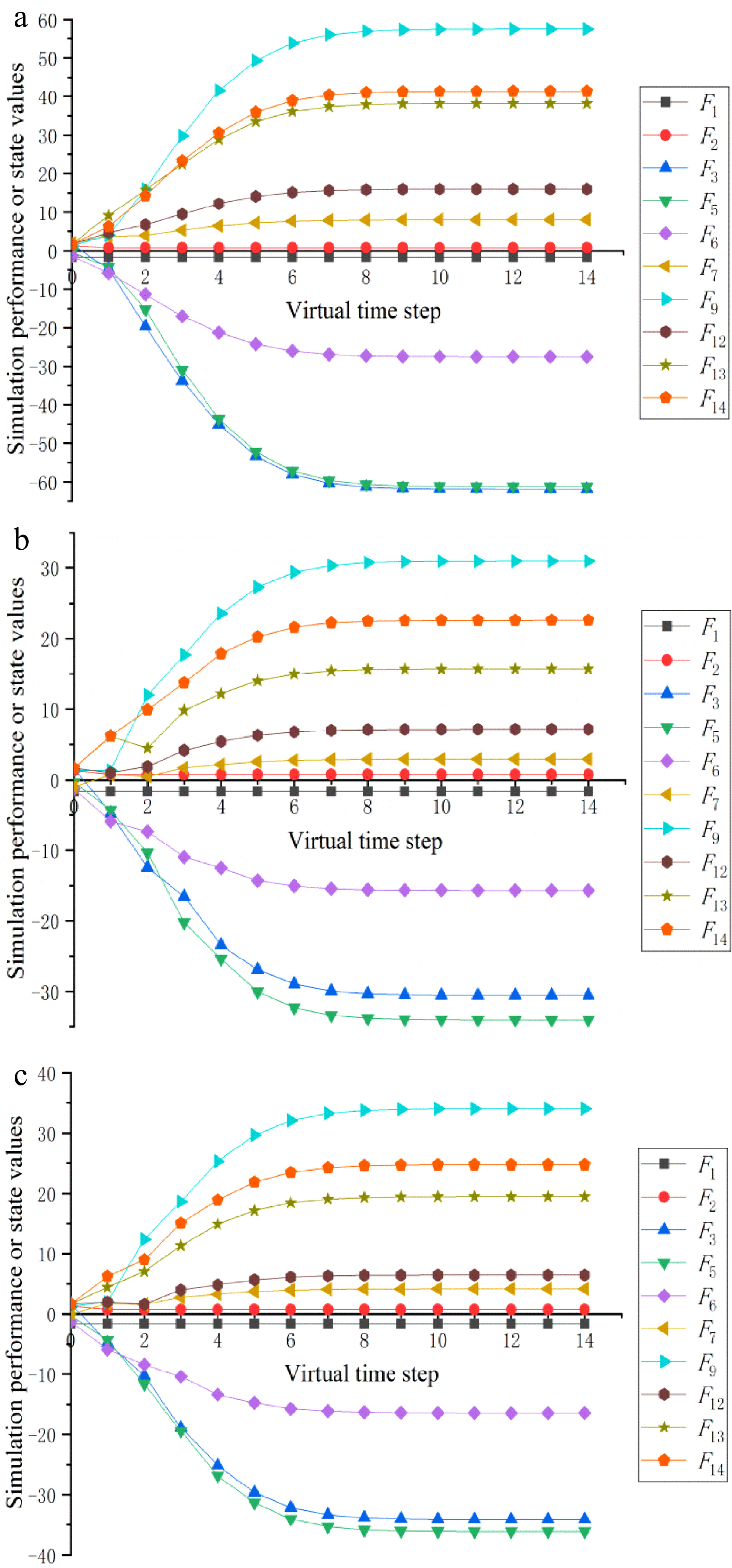
Figure 5. 

Evolutions of simulation performance or state values of factors of emergency scenarios $ {{\hat e}}_1^{{{{t}}_2}} $, $ {{\hat e}}_2^{{{{t}}_2}} $ and $ {{\hat e}}_3^{{{{t}}_2}} $. (a) for $ {{\hat e}}_1^{{{{t}}_2}} $; (b) for $ {{\hat e}}_2^{{{{t}}_2}} $; (c) for $ {{\hat e}}_3^{{{{t}}_2}} $.

The above case analysis results can guide DMs in emergency management departments to determine critical factors of disaster management that have greater weights, such $ {{{F}}_6} $, $ {{{F}}_9} $, $ {{{F}}_{10}} $ at $ {{{t}}_1} $ and $ {F_3} $, $ {F_5} $, $ {F_9} $, $ {F_{13}} $ at $ {{{t}}_2} $. Meanwhile, classified management of factors can be implemented according to the cause-effect classification graphically described in the causal diagram. More importantly, the simulation processes help DMs comprehend the potential development of disaster under different emergency response measures. Based on simulation results, DMs can figure out which emergency response measure will yield the most desired outcome of disaster management, and thus make effective emergency decision making.

This section presents a comparative analysis between the outcomes obtained by the extended DEMATEL method and traditional DEMATEL method. For a valid comparison, bipolar linguistic evaluation information used in the proposed method is converted into crisp numbers for implementing DEMATEL method, where the absolute value is adopted as the traditional DEMATEL method doesn’t distinguish the positiveness and negativeness of influence among factors. Analogous to Step 12 of the proposed method, to calculate the simulation performance or state values $ {{{R}}^{{D}}} = [\xi _1^{{D}},\xi _2^{{D}},...,\xi _n^{{D}}] $ of factors according to the DEMATEL method, the following equation is used:

where $ {{{T}}^{{D}}} $ is the total relation matrice derived by the DEMATEL method.

Following the above operations, the classical DEMATEL method is applied to solve the same evaluation problem described in Section "Illustrative Example". The results are displayed in Table 4.

From Table 4 and the results obtained by the proposed method, it can be seen that despite some differences in the overall performance values between the two methods, it shows that the introduction of clearing roadblocks and evacuating traffic by the traffic department in $ {{\hat e}}_2^{{{{t}}_1}} $ at $ {{{t}}_1} $ and the state of $ {F_7} $ and its influences exerted to other factors in $ {{\hat e}}_1^{{{{t}}_2}} $ at $ {{{t}}_2} $ are more beneficial for disaster management than other scenarios. This finding, to some extent, validates the outcome obtained by the proposed method. However, taking a closer look, more significant findings can be obtained.

Regarding the factor weights, it can be observed that the weight values of factors obtained by the two methods are different for all the emergency scenarios. By DEMATEL, the top three important factors for $ {{\hat e}}_1^{{{{t}}_1}} $ and $ {{\hat e}}_2^{{{{t}}_1}} $ are $ {{{F}}_1} $, $ {{{F}}_3} $, $ {{{F}}_9} $ and $ {{{F}}_1} $, $ {{{F}}_6} $, $ {{{F}}_9} $, respectively, which lay emphasis on the rescue and the effect of typhoon and leakage. Nevertheless, the suggested method derives the top three critical factors as $ {{{F}}_6} $, $ {{{F}}_9} $, $ {{{F}}_{10}} $ for both $ {{\hat e}}_1^{{{{t}}_1}} $ and $ {{\hat e}}_2^{{{{t}}_1}} $ that coincides with the main object of rescue and evacuation at time point $ {{{t}}_1} $ and thus is more logical for disaster management. For all three emergency scenarios at time point $ {{{t}}_2} $, although factors owning greater importance are $ {F_3} $, $ {F_5} $, $ {F_9} $ and $ {F_{13}} $ according to both methods, the weights of factors for three different scenarios $ {{\hat e}}_1^{{{{t}}_2}} $, $ {{\hat e}}_2^{{{{t}}_2}} $ and $ {{\hat e}}_3^{{{{t}}_2}} $ acquired via DEMATEL are almost the same. This suggests the traditional DEMATEL method fails to effectively distinguish the effects of factor $ {F_7} $ with different states, compared with the proposed method.

Besides, it can be seen that the cause-effect classification of factors obtained by the two methods are also different for all the emergency scenarios. For scenarios at $ {{{t}}_1} $, $ {{{F}}_1} $, $ {{{F}}_2} $, $ {{{F}}_3} $ are classified as cause factors by DEMATEL, which echoes the previous analysis that the results put more emphasis on the effect of typhoon and leakage and deviate from the main object of time point $ {{{t}}_1} $. For scenarios at $ {{{t}}_2} $, the cause-effect classifications obtained by the two methods are the same, however, the net effects and net causes of factors by DEMATEL for different scenarios have small differences, especially for $ {{\hat e}}_2^{{{{t}}_2}} $ and $ {{\hat e}}_3^{{{{t}}_2}} $. This indicates that the interrelationships among factors produced by DEMATEL do not display the influences of different states and different direct relations with other factors of $ {F_7} $.

Based on the above analysis and the different characteristics of these two methods, it is evident that the differences between outcomes of the proposed method and the DEMATEL method are mainly because the DEMATEL method only captures the strengths of direct relations among factors, whereas the proposed method can not only capture the strength of influence but also the kind of influence, namely positive influence or negative influence. From the considered example, it can be seen that different types of influences do exist among influential factors in actual disaster management. Also, the proposed method, considering the positiveness and negativeness of influence produces more reasonable and practical assessment results. Moreover, since the inputs of DEMATEL are transformed from those of the advised method without value loss, no differences between results are observed caused by different evaluation information modelling. But, the proposed method represents the assessments by bipolar 2-tuple linguistic variables, which can effectively manage the fuzziness and uncertainty of assessment objects in complex emergencies and make experts feel more comfortable in providing assessments than using numeric values.

Since destructive disasters frequently occur, it is important to enhance disaster management. In this study, a dynamic interaction assessment method for disaster management based on the extended DEMATEL is proposed. By taking advantage of bipolar 2-tuple linguistic variables, the proposed method can exactly process vague and uncertain linguistic evaluations. Also, both the positive and negative influences among factors involved in dealing with the disaster are well modeled. The extended DEMATEL effectively dissects the complex causal relationships and roles played in disaster management of influential factors. Additionally, the suggested simulation process can present the dynamic evolutions of factors and different emergency scenarios, which offers valuable information about emergency scenario evolution after taking response measures. An illustrative example of liquefied petroleum gas leakage caused by a typhoon is given to demonstrate the practicability and effectiveness of the approach, together with a comparative analysis between the suggested method and the traditional DEMATEL method. It was shown that the recommended method is a useful means to capture the causality among influential factors and explore how these factors and their interactions affect disaster management. The simulation results enable forward-thinking insight into emergency response, based on which the emergency management department can assess the effectiveness of emergency measures and the possible evolution trend of disasters, and further manage the disaster more scientifically.

As for future work, the suggested method will be modified to handle the multi-source information since the performances or states of some influential factors may be described quantitatively after more disaster information available. Moreover, because of disaster management covering a series of activities, it is favorable to incorporate group decision making into the proposed method for conducting more credible evaluations. Also, the proposed method will be further extended by considering the bounded rationality of DMs or experts under risk and uncertainty by virtue of the prospect theory.