


-
Providing reliable electricity to meet society's needs is a major concern for countries globally. However, aging infrastructure and the increasing frequency of natural disasters pose significant threats to the stability of power systems. The electricity crisis in Pakistan serves as a prominent example of how supply deficits and vulnerabilities in the power grid can escalate into major political and socioeconomic issues[1]. Consequently, reliable assessment of the resilience of energy infrastructure to natural disasters is a paramount concern for researchers, government officials, and community members.
Resilience refers to the ability of a system to withstand, adapt to, and rapidly recover from disruptive events. Recent studies have established comprehensive frameworks for resilience-based infrastructure planning, particularly in the context of water distribution systems and urban sustainability[2]. Though metrics for resilience are evolving, the sensitivity of electric power infrastructure to the spatial distribution of disaster impacts creates significant uncertainty in recovery predictions[3]. Furthermore, given the high interdependency of critical infrastructure, joint restoration modeling has become essential for realistic resilience assessments[4]. These assessments are critical under extreme weather conditions, such as typhoons, where regulatory and operational frameworks are tested to their limits[5].
To enhance resilience, researchers have proposed various enhancement strategies. These range from robust optimization-based planning that incorporates distributed generation to mitigate the impact of natural disasters[6,7] through to dynamic operational strategies and mobile energy storage systems[8]. Strengthening the infrastructure against specific hazards remains a primary strategy, with studies quantifying the benefits of vegetation management and reinforcement strategies[9]. Insights from other critical infrastructure, such as telecommunications, further highlight the importance of post-disaster site surveys and the fragility of power plants during events like Hurricane Katrina[10]. Additionally, utility outage statistics have been utilized to quantify improvements in bulk power systems' resilience, emphasizing the need for data-driven approaches[11].
A key component of operational resilience is asset management. Effective management of asset performance within power grids is crucial for maintaining service quality[12]. This involves trade-offs between costs and reliability, such as the decision to invest in underground versus overhead lines[13]. Integrating risk analyses with multi-criteria decision support is a common approach in electricity distribution system-related asset management to prioritize investments[14]. Previous studies have also explored asset management models for specific equipment, such as public lighting systems, to evaluate economic performance[15]. Furthermore, recent research has highlighted the economic sustainability of asset management, analyzing the stability of repair activities and the impact of load growth and inflation on long-term planning in metropolitan grids[16].
Despite these advancements in resilience planning and economic asset management, a significant void remains in the quantitative modeling of pre-disaster warehousing for crisis scenarios. Most existing asset management models focus on steady-state reliability or long-term lifecycle costs. However, during high-impact–low-probability (HILP) events, the simultaneous failure of assets creates an immediate, massive demand for spare parts that conventional reliability models fail to predict. There is a lack of a practical, data-driven framework that directly integrates engineering fragility curves with real-world asset lifecycle data to optimize crisis inventories. Although economic models address the stability of routine repairs[17], they do not quantify the precise number of assets required in the warehouse to withstand HILP events with various levels of severity.
To address this research gap, this paper proposes a data-driven decision-support framework for emergency resource management in critical infrastructure. By integrating engineering fragility curves with a unique 10-year operational dataset, our model quantifies the precise number of asset failures required to ensure the rapid restoration of services. The primary contributions of this paper are threefold.
(1) It integrates engineering risk models with real-world asset data to create a scientific tool for strategic resource allocation.
(2) It provides a quantitative model for optimizing crisis warehousing, a key component of emergency logistics, by calibrating fragility curves using historical failure data.
(3) It presents a validated case study using data from the Tehran Regional Electric Distribution Company (TREDC), demonstrating how this technology can be leveraged by emergency managers to enhance resilience, providing a blueprint for other sectors.
-
To optimize emergency resource management, we propose a framework that integrates engineering fragility models with asset lifecycle dynamics. The modeling process is divided into three key steps: (1) data-driven fragility curve calibration, (2) asset lifetime integration, and (3) spare asset quantification.
As can be seen in Fig. 1, every asset in the normal state has an average failure probability
$ {P}_{\lambda } $ 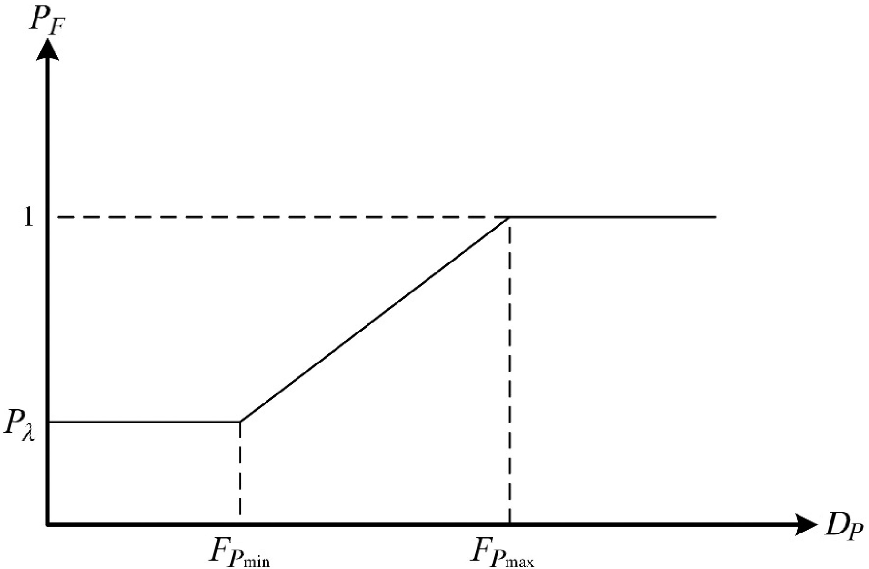
Figure 1.
Conceptual asset fragility curve illustrating failure probability as a function of HILP event severity.
The mathematical framework presented in this study is developed on the basis of the first principles of reliability engineering and asset management theory. The linear fragility model (Eqs. 1–6) is adopted as a simplified approximation of hazard susceptibility commonly used in infrastructure risk assessment[18], whereas the dynamic lifecycle matrix derivation (Eqs. 7–20) is an original contribution of this research, formulated to explicitly track assets' aging under network expansion and depreciation rates.
$ {P}_{F}=\dfrac{1-{P}_{\lambda }}{{{{F}_{P}}}_{max}-{{{F}_{P}}}_{min}}\left({D}_{P}-{{{F}_{P}}}_{min}\right)+{P}_{\lambda } $ (1) where, FPmin is the wind speed threshold where failures begin, and FPmax is the wind speed at which total failure is expected.
If we assume that N assets are exposed to the HILP incident, the number of failures is obtained via Eq. (2).
$ N_{w}^{({D}_{P})}=\left[\dfrac{1-{P}_{\lambda }}{{{{F}_{P}}}_{max}-{{{F}_{P}}}_{min}}\left({D}_{P}-{{{F}_{P}}}_{min}\right)+{P}_{\lambda }\right]\times N $ (2) As the total
$ N_{w}^{({D}_{P})} $ 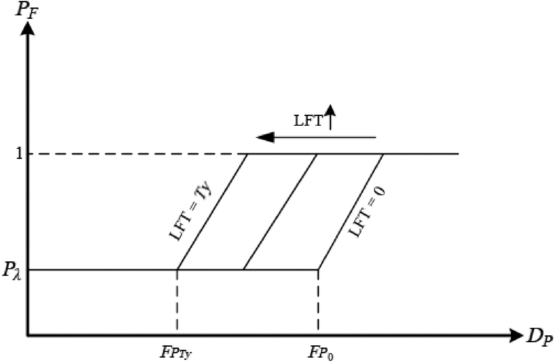
Figure 2.
The impact of asset lifetime on fragility curves, illustrating reduced resilience in older assets.
It is obvious that for each lifetime,
$ {{{F}_{P}}}_{max}> \gt {{{F}_{P}}}_{min} $ $ {{{F}_{P}}}_{max}\left({T}_{y}\right) \gt {{{F}_{P}}}_{min}\left(0\right) $ (3) As shown in Fig. 2, the slope of the fragility curve is assumed to be the same across different lifetimes. For modeling simplicity and based on a preliminary analysis of the company's failure records, which did not show a statistically significant variation in the failure rate slope across different asset age groups, this assumption was made. Moreover, as the lifetime expectancy increases, the asset's resistance to HILP events decreases, and it is damaged at lower accident intensities. Thus, if the relationship between the severity of the accident at the point of failure (FP) is plotted in terms of lifetime, Fig. 3 is obtained.
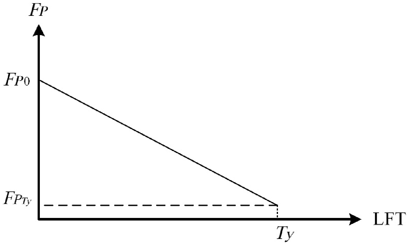
Figure 3.
Linearized relationship between asset lifetime and the failure point (FP) severity.
Linearizing FP and LTF yields Eq. (4).
$ \dfrac{{{{F}_{P}}}_{0-}{{{F}_{P}}}_{Ty}}{0-{T}_{y}}=\dfrac{{{{F}_{P}}}_{0-}{F}_{P}}{0-LTF}{\Rightarrow}{ }{F}_{P}\left(LFT\right)={{{F}_{P}}}_{0}-\left({{{F}_{P}}}_{0}-{{{F}_{P}}}_{{{T}_{y}}}\right)LFT $ (4) If the number of assets is calculated over different lifetimes, the number of failures is calculated using Eq. (5).
$ {N}_{W}=\sum{P}_{F}(LTF){n}_{LTF} $ (5) $ {P}_{F} $ $ {P}_{F}\left(LTF\right)=\left\{\begin{array}{cc} {P}_{\lambda } & {F}_{P} \lt {{{F}_{P}}}_{min}\\ \dfrac{1-{P}_{\lambda }}{{{{F}_{P}}}_{max}-{{{F}_{P}}}_{min}}{F}_{P}\left(LFT\right)+{P}_{\lambda } & {{{F}_{P}}}_{min}\leq {F}_{P}\leq {F}_{{{P}_{max}}}\\ 1 & {F}_{P} \lt {{{F}_{P}}}_{max} \end{array}\right\} $ (6) In this way, the flowchart (Fig. 4) for calculating the number of failures and the required spare parts in the warehouse was determined.
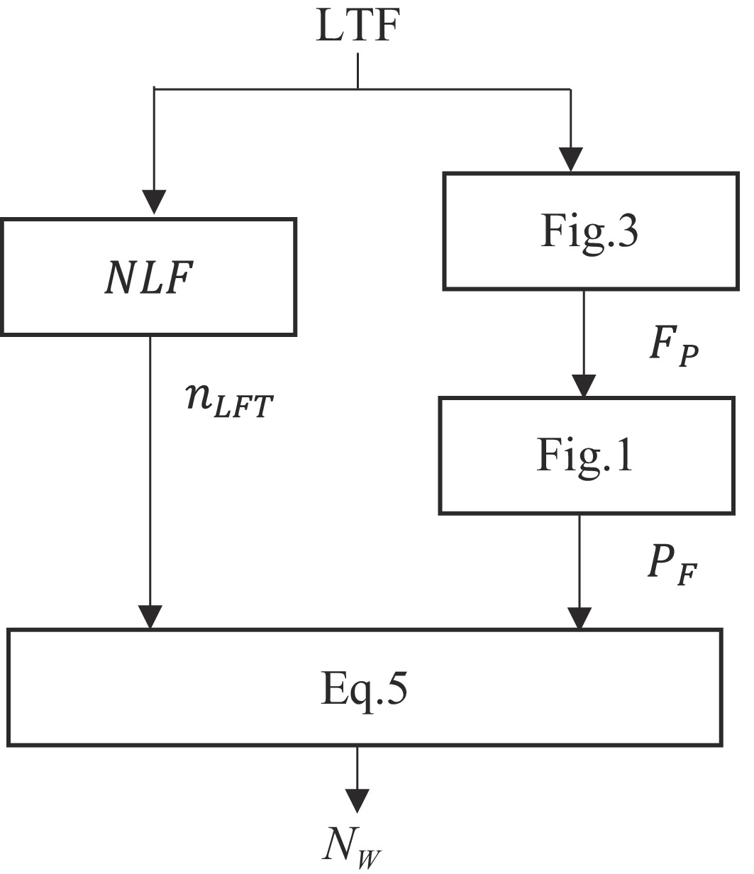
Figure 4.
Flowchart of the proposed model for calculating the required spare assets in the crisis warehouse.
NLF is the number of assets in each lifetime, which can be calculated by understanding the development and failure process as follows. If k is the base year and k = 0 is the base year of the electricity industry, the development process can be plotted in Table 1.
Table 1. Matrix representation of asset count by lifetime (j) and year (k), considering only annual development.
k j 0 1 2 3 0 $ N $ 1 $ aN $ $ N $ 2 $ a(1+a)N $ $ aN $ $ N $ 3 $ a({1+a)}^{2}N $ $ a(1+a)N $ $ aN $ $ N $ Table 1 is based on equalizing assets (1 + a) each year as the distribution network's assets develop. This table shows the number of assets with different lifetimes in year k of the electricity industry, assuming that the number of assets at the origin is N and the load growth is a. In this case, the number of j-year assets in the electricity industry in year K can be calculated using Eq. (7).
$ {n}_{kj}=a{(1+a)}^{k-j-1}\times N $ (7) However, the depreciation rate of assets is not included in Eq. (7). To consider this parameter, Table 2 is based on the failure rate λ, which is multiplied by the annual assets and rewritten.
Table 2. Matrix representation of asset count by lifetime (j) and year (k) considering both annual development and failure rate (λ).
k j 0 1 2 3 0 $ N $ 1 $ (a+\lambda )N $ $ (1-\lambda )N $ 2 $ (a+\lambda )(1+a)N $ $ (a+\lambda )(1-\lambda )N $ $ {(1-\lambda )}^{2}N $ 3 $ (a+\lambda )({1+a)}^{2}N $ $ (a+\lambda )(1+a)(1-\lambda )N $ $ {(a+\lambda )(1-\lambda )}^{2}N $ $ {(1-\lambda )}^{3}N $ Thus, the number of j-year assets in year k is calculated via Eq. (8).
${n}_{kj}=\left(a+\lambda \right){\left(1+a\right)}^{k-j-1}{\left(1-\lambda \right)}^{j}N $ (8) The n_k0 array must be used to find the number of assets required for the development warehouse. Assuming balanced development throughout the year, there are always
$ \dfrac{{n}_{k0}}{12} $ $ {nY}_{D}=\left(a+\lambda \right){\left(1+a\right)}^{k-1}N={n}_{k0} $ (9) The total available asset is a reliable indicator. Given the load growth rate and failure rate of assets, the number of assets with different lifetimes can be expressed as a simple function of the total number of available assets. For this purpose, based on Eq. (8), a matrix is considered as shown in Eq. (10).
$ Assets=\left[\begin{array}{ccc} \begin{array}{c} N\\ \left(a+\lambda \right)N\\ \begin{array}{c} \left(a+\lambda \right)\left(1+a\right)N\\ \ldots \\ \left(a+\lambda \right){\left(1+a\right)}^{m-1}N \end{array} \end{array} & \begin{array}{c} 0\\ \left(1-\lambda \right)N\\ \begin{array}{c} \left(a+\lambda \right)\left(1-\lambda \right)N\\ \ldots \\ \left(a+\lambda \right){\left(1+a\right)}^{m-2}\left(1-\lambda \right)N \end{array} \end{array} & \begin{array}{ccc} \begin{array}{c} 0\\ 0\\ \begin{array}{c} {\left(1-\lambda \right)}^{2}N\\ \ldots \\ \left(a+\lambda \right){\left(1+a\right)}^{m-3}{\left(1-\lambda \right)}^{2}N \end{array} \end{array} & \begin{array}{c} \ldots \\ \ldots \\ \begin{array}{c} \ldots \\ \ldots \\ \ldots \end{array} \end{array} & \begin{array}{c} 0\\ 0\\ \begin{array}{c} 0\\ \ldots \\ {\left(1-\lambda \right)}^{m}N \end{array} \end{array} \end{array} \end{array}\right] $ (10) where, M is the number of years in the electricity industry from the base year, as can be seen;
$ {n}_{{{k}_{0}}} $ $ \dfrac{1}{12} $ $ \dfrac{{n}_{kj}}{{n}_{\left(k-1\right)j}}=1+a $ (11) $ \dfrac{{n}_{kj}}{{n}_{k(j-1)}}=\dfrac{1-\lambda }{1+a} $ (12) This matrix represents the dynamic lifecycle of assets, accounting for annual load growth (
$ a $ $ \lambda $ Equation (11) shows the same relation of
$ {n}_{kj} $ $ {n}_{kj} $ $ {\left(1+a\right)}^{k}N $ $ {NOA}_{m}=\sum\limits_{j=1}^{m-1}(a+\lambda ){\left(1+a\right)}^{m-j-1}{(1-\lambda )}^{j}N+{(1-\lambda )}^{m}N={(1+a)}^{m}N $ (13) As can be seen from the asset matrix in Eq. (10), each
$ {n}_{kj} $ 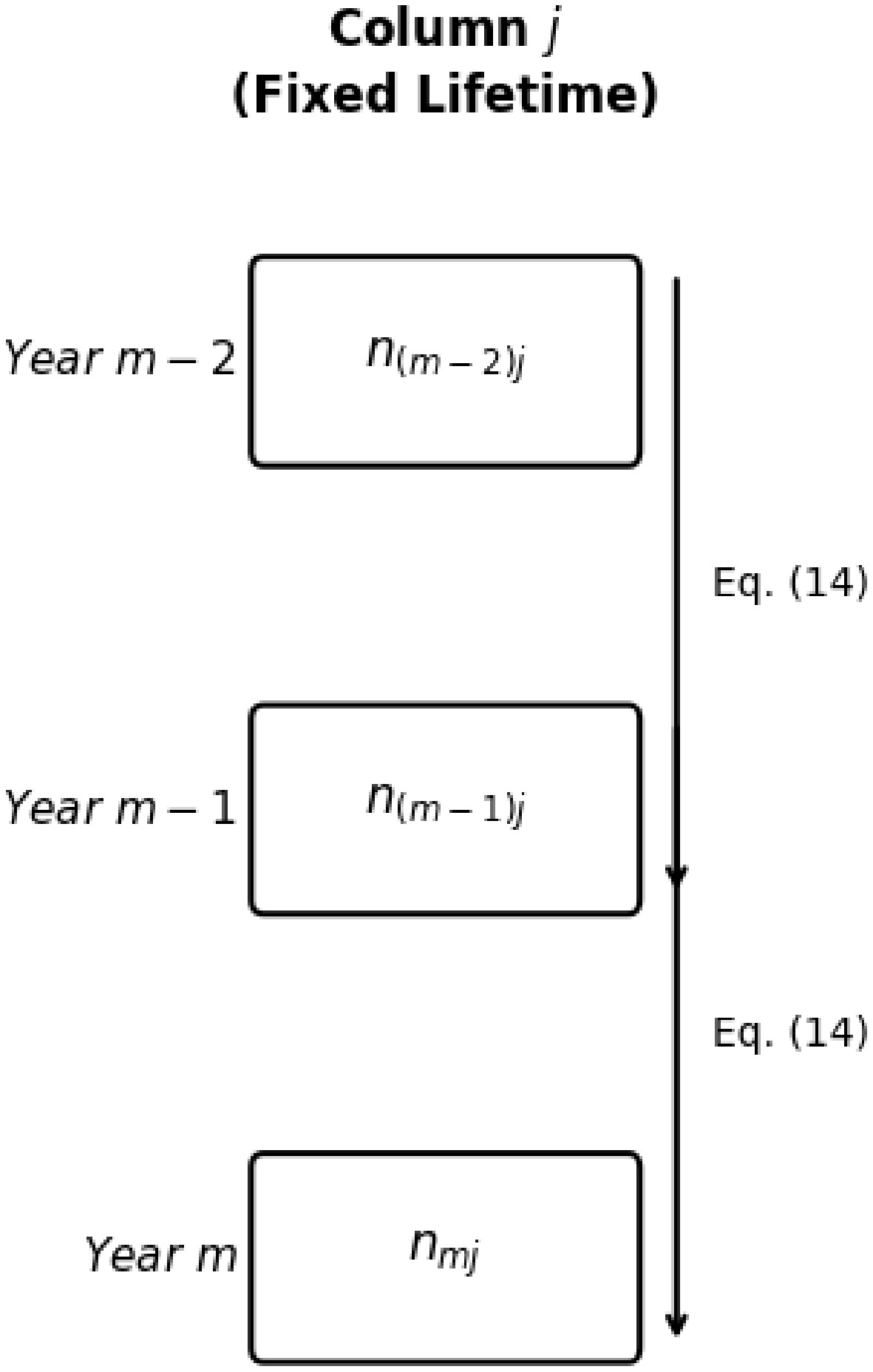
Figure 5.
Schematic of the column-wise relationships within the asset matrix.
$ {n}_{\left(m-1\right)j}=\dfrac{{n}_{mj}}{\left(1+a\right)}\;\;\;{n}_{\left(m-2\right)j}=\dfrac{{n}_{(m-1)j}}{\left(1+a\right)}=\dfrac{{n}_{mj}}{{(1+a)}^{2}} $ (14) Generally, we have
$\forall j \lt k \lt m;\;\;{n}_{kj}=\dfrac{{n}_{mj}}{{\left(1+a\right)}^{m-k}} $ (15) Equation (15) shows the j-year assets in year k as a percentage of the j-year assets in year m for the electricity industry. In this way, the lifetimes of future years' assets are predictable. Figure 6 shows the row relation of the assets matrix. Using Fig. 6 and Eq. (4), Eqs (16)−(19) are obtained.

Figure 6.
Schematic of the row-wise relationships within the asset matrix.
$ {n}_{mj}=\dfrac{1-\lambda }{1+a}{n}_{m(j-1)} $ (16) As a result, we have
$ {n}_{m1}=\dfrac{1-\lambda }{1+a}{n}_{m0} ,\;\; {n}_{m2}=\dfrac{1-\lambda }{1+a}{n}_{m1}=\left(\dfrac{1-\lambda }{1+a}\right)^{2}{n}_{m0} $ (17) Generally, the number of assets with different lifetimes related to the development rate of year m can be written as shown in Eq. (18):
$ {\forall 0 \lt j\leq m\colon n}_{mj}=\left(\dfrac{1-\lambda }{1+a}\right)^{j}{n}_{m0} $ (18) On the other hand, using Eqs (8) and (13), the amount of annual development can be related to the number of available assets, as shown in Eq. (19).
$ \dfrac{{n}_{m0}}{{NOA}_{m}}=\dfrac{(\lambda +a){(1+a)}^{m-1}N}{{(1+a)}^{m}N}=\dfrac{\lambda +a}{1+a} $ (19) Using Eq. (19), the number of assets with lifetime j can be written as in Eq. (20).
$ {n}_{mj}=\left(\dfrac{1-\lambda }{1+a}\right)^{j}\cdot\dfrac{\lambda +a}{1+a} . {NOA}_{m} $ (20) Equation (20) shows the number of assets with different lifetimes, which is formulated as the total number of available assets. Thus, the NLF relation in Fig. 4 can be represented as shown in Eq. (20). Therefore, NW can easily be calculated.
-
This study utilizes a comprehensive dataset from TREDC spanning 10 years (2013–2022).
Case study and data description
-
The dataset contains detailed records of 50,000 distribution transformers and poles. It includes installation dates (for calculating lifetimes), failure logs with timestamps, and maintenance records. Meteorological data, specifically wind speed records, were obtained from the Iran Meteorological Organization. By spatially and temporally matching failure events with storm intensities, we were able to extract the fragility parameters (Dpmin, Dpmax) for different asset age groups, as detailed in Table 3. According to Eq. (5), the number of assets during different lifetimes is presented in the form of Table 4.
Table 3. Extracted fragility parameters (Dpmin, Dpmax) for assets of varying lifetimes based on TREDC historical data.
LFT Dpmin Dpmax LFT Dpmin Dpmax 1 120 250 16 90 175 2 118 245 17 88 170 3 116 240 18 86 165 4 114 235 19 84 160 5 112 230 20 82 155 6 110 225 21 80 150 7 108 220 22 78 145 8 106 215 23 76 140 9 104 210 24 74 135 10 102 205 25 72 130 11 100 200 26 70 125 12 98 195 27 68 120 13 96 190 28 66 115 14 94 185 29 64 110 15 92 180 30 62 105 As shown in Table 3, the calibration results confirm that older assets have significantly lower failure thresholds (Dpmin, Dpmax), validating the degradation model.
As shown in Table 4 and Fig. 7, even at low wind speeds (50−70 km/h), a baseline number of asset failures is predicted. The number of damaged assets, which directly translates to the quantity of spare parts required for storage, increases significantly with higher storm intensities. This quantification allows managers to move from qualitative risk assessment to a data-driven budgeting process for spare parts.
Table 4. Calculated number of damaged assets (Nw), required spare Assets (Pw), and percentage of total assets (PRC) at various storm wind speeds (DP).
DP Nw Pw PRC DP Nw Pw PRC 50 80.18882 11.53376 0.576688 160 473.0745 68.04348 3.402174 60 80.18882 11.53376 0.576688 170 516.2171 74.24878 3.712439 70 84.36561 12.13452 0.606726 180 555.1179 79.84399 3.992199 80 98.71709 14.19872 0.709936 190 589.6541 84.81142 4.240571 90 123.2898 17.73308 0.886654 200 619.6781 89.12985 4.456492 100 158.6401 22.8176 1.14088 210 645.0183 92.77459 4.63873 110 204.6656 29.43757 1.471878 220 665.479 95.7175 4.785875 120 259.5956 37.33828 1.866914 230 680.8398 97.92688 4.896344 130 319.0274 45.8865 2.294325 240 690.8552 97.92688 4.968371 140 374.4256 53.85456 2.692728 250 695.2532 100 5 150 425.7875 61.24207 3.062103 260 695.2532 100 5 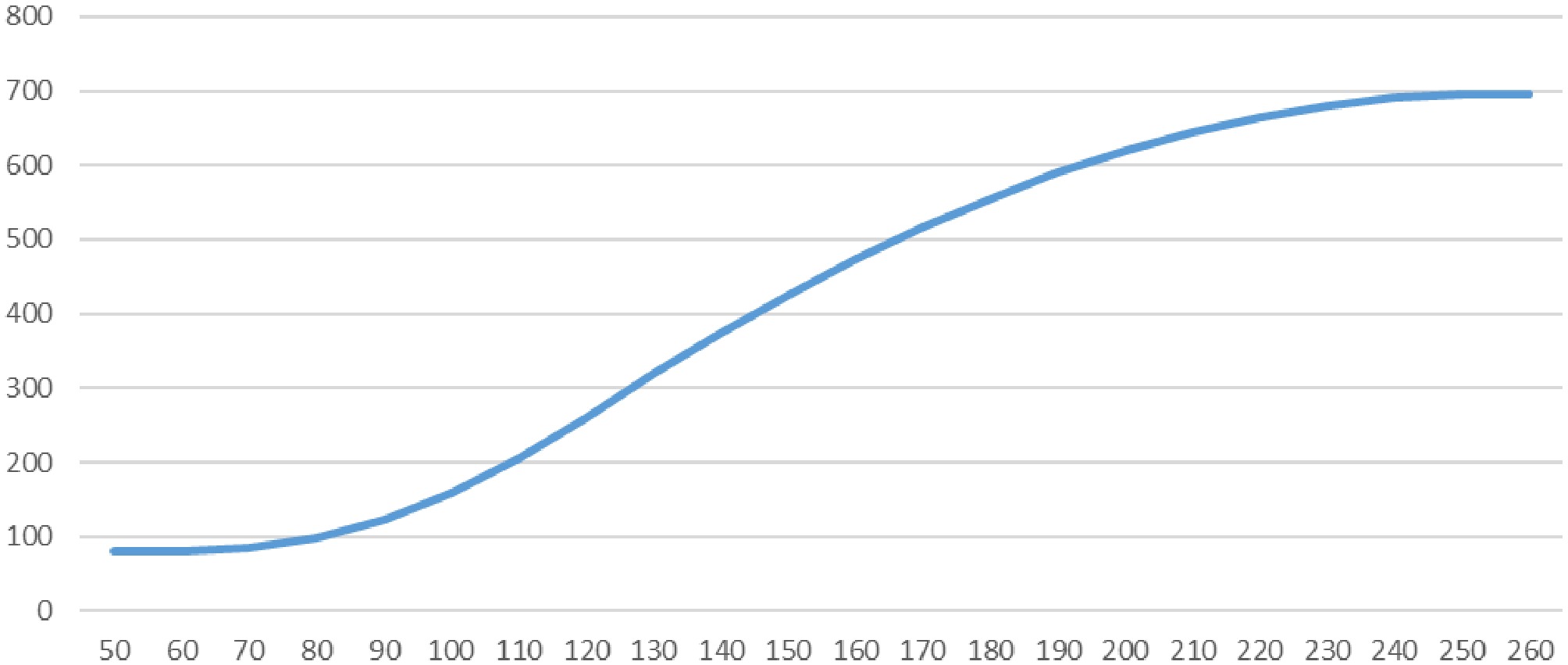
Figure 7.
Estimated number of damaged assets vs. storm wind speed, based on the TREDC dataset.
The model's output represents the total number of assets required for the crisis warehouse. However, this quantity can be offset by the assets available in the development warehouse. According to TREDC's operational data, the development warehouse consistently maintains an average of 100 spare assets for routine projects. These assets can be temporarily reallocated during a major HILP event, effectively reducing the required inventory for the crisis warehouse by this amount. Furthermore, the expansion of decentralized generation and mobile emergency units can mitigate the impact of asset failures, though this effect is not quantified in the current model. The relationship between asset growth and the required number of spares is critical. As shown in Table 5 and Fig. 8, a higher asset growth rate (coefficient a) leads to a larger proportion of younger, more resilient assets, which, in turn, reduces the overall number of predicted failures for an event with a given level of severity.
Table 5. Sensitivity analysis: Asset count by lifetime for different load growth rates (a) from 0.01 to 0.05.
Number of assets
by lifetimeAsset growth rate (a) 0.01 % 0.02 % 0.03 % 0.04 % 0.05 % 1 1,000 1 1,000 1 1,000 1 1,000 1 1,000 1 2 980.198 0.980198 970.588 0.970588 961.165 0.961165 951.923 0.951923 942.857 0.942857 3 960.788 0.960788 942.042 0.942042 923.838 0.923838 906.158 0.906158 888.98 0.88898 4 941.763 0.941763 914.334 0.914334 887.961 0.887961 862.592 0.862592 838.181 0.838181 5 923.114 0.923114 887.442 0.887442 853.477 0.853477 821.122 0.821122 790.285 0.790285 6 904.834 0.904834 861.341 0.861341 820.332 0.820332 781.645 0.781645 745.126 0.745126 7 886.917 0.886917 836.007 0.836007 788.475 0.788475 744.065 0.744065 702.547 0.702547 8 869.354 0.869354 811.419 0.811419 757.854 0.757854 708.293 0.708293 662.401 0.662401 9 852.139 0.852139 787.554 0.787554 728.423 0.728423 674.241 0.674241 624.55 0.62455 10 835.265 0.835265 764.39 0.76439 700.135 0.700135 641.825 0.641825 588.861 0.588861 11 818.725 0.818725 741.908 0.741908 672.945 0.672945 610.968 0.610968 555.212 0.555212 12 802.513 0.802513 720.088 0.720088 646.811 0.646811 581.595 0.581595 523.486 0.523486 13 786.622 0.786622 698.908 0.698908 621.693 0.621693 553.633 0.553633 493.572 0.493572 14 771.045 0.771045 678.352 0.678352 597.549 0.597549 527.016 0.527016 465.368 0.465368 15 755.777 0.755777 658.401 0.658401 574.343 0.574343 501.679 0.501679 438.776 0.438776 16 740.811 0.740811 639.036 0.639036 552.039 0.552039 477.56 0.47756 413.703 0.413703 17 726.141 0.726141 620.241 0.620241 530.6 0.5306 454.6 0.4546 390.063 0.390063 18 711.762 0.711762 601.999 0.601999 509.995 0.509995 432.745 0.432745 367.773 0.367773 19 697.668 0.697668 584.293 0.584293 490.189 0.490189 411.94 0.41194 346.758 0.346758 20 683.853 0.683853 567.108 0.567108 471.152 0.471152 392.135 0.392135 326.943 0.326943 21 670.311 0.670311 550.428 0.550428 452.855 0.452855 373.282 0.373282 308.261 0.308261 22 657.038 0.657038 534.239 0.534239 435.269 0.435269 355.336 0.355336 290.646 0.290646 23 644.027 0.644027 518.526 0.518526 418.365 0.418365 338.252 0.338252 274.037 0.274037 24 631.274 0.631274 503.275 0.503275 402.118 0.402118 321.99 0.32199 258.378 0.258378 25 618.774 0.618774 488.473 0.488473 386.502 0.386502 306.51 0.30651 243.614 0.243614 26 606.521 0.606521 474.106 0.474106 371.492 0.371492 291.774 0.291774 229.693 0.229693 27 594.51 0.59451 460.162 0.460162 357.065 0.357065 277.746 0.277746 216.568 0.216568 28 582.738 0.582738 446.628 0.446628 343.198 0.343198 264.393 0.264393 204.192 0.204192 29 571.198 0.571198 433.492 0.433492 329.87 0.32987 251.682 0.251682 192.524 0.192524 30 559.888 0.559888 420.742 0.420742 317.06 0.31706 239.582 0.239582 181.523 0.181523 Total 22,785.6 22.78557 20,115.5 20.11552 17,902.8 17.90277 16,056.3 16.05628 14,504.9 14.50488 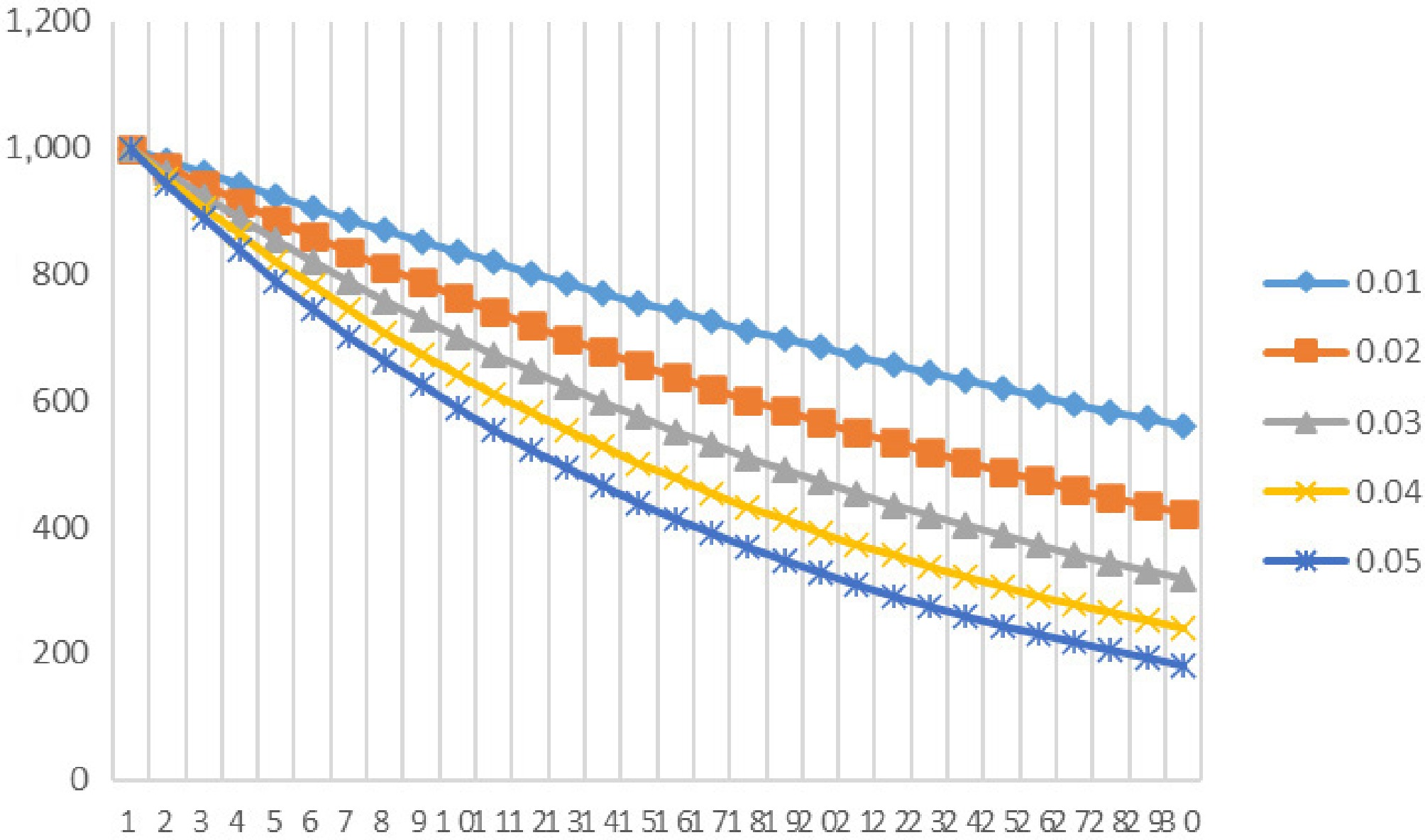
Figure 8.
Distribution of asset count by lifetime for various annual load growth rates (a) from 0.01 to 0.05.
Table 6 and Fig. 9 illustrate the impact of the asset growth rate (a) on the absolute number of damaged assets. A critical insight emerges here: Although a higher growth rate results in a larger proportion of younger, more resilient assets (improving the inventory's average resistance), it also increases the total asset base. Consequently, the absolute number of assets exposed to the hazard rises, leading to a higher number of failures for an event with a given level of severity. This clarifies that network expansion must be accompanied by a proportional scaling of emergency inventory to maintain a constant level of service resilience.
Table 6. Sensitivity analysis: Number of damaged assets at various storm severities for different load growth rates (a).
Number of assets damaged in the
different accident severitiesAsset growth rate (a) 0.01 % 0.02 % 0.03 % 0.04 % 0.05 % 60 16.04 0.01604 32.08 0.03208 48.11 0.04811 64.15 0.06415 80.2 0.0802 70 16.87 0.01687 33.75 0.03375 50.62 0.05062 67.49 0.06749 84.37 0.08437 80 19.74 0.01974 39.49 0.03949 59.23 0.05923 78.97 0.07897 98.72 0.09872 90 24.66 0.02466 49.32 0.04932 73.97 0.07397 98.63 0.09863 123.29 0.12329 100 31.73 0.03173 63.46 0.06346 95.18 0.09518 126.91 0.12691 158.64 0.15864 110 40.93 0.04093 81.87 0.08187 122.8 0.1228 163.73 0.16373 204.67 0.20467 120 51.92 0.05192 103.84 0.10384 155.76 0.15576 207.68 0.20768 259.6 0.2596 130 63.81 0.06381 127.61 0.12761 191.42 0.19142 255.22 0.25522 319.03 0.31903 140 74.86 0.07486 149.77 0.14977 224.66 0.22466 299.54 0.29954 374.43 0.37443 150 85.16 0.08516 170.31 0.17031 255.47 0.25547 340.63 0.34063 425.79 0.42579 160 94.61 0.09461 189.23 0.18923 283.85 0.28385 378.46 0.37846 473.07 0.47307 170 103.24 0.10324 206.49 0.20649 309.73 0.30973 412.97 0.41297 516.22 0.51622 180 111.02 0.11102 222.05 0.22205 333.07 0.33307 444.09 0.44409 555.12 0.55512 190 117.93 0.11793 235.86 0.23586 353.79 0.35379 471.72 0.47172 589.65 0.58965 200 123.94 0.12394 247.87 0.24787 371.81 0.37181 495.74 0.49574 619.68 0.61968 210 129 0.129 258.01 0.25801 387.01 0.38701 516.01 0.51601 645.02 0.64502 220 133.1 0.1331 266.19 0.26619 399.29 0.39929 532.38 0.53238 665.48 0.66548 230 136.17 0.13617 272.34 0.27234 408.5 0.4085 544.67 0.54467 680.84 0.68084 240 138.17 0.13817 276.34 0.27634 414.51 0.41451 552.684 0.552684 690.86 0.69086 250 139.05 0.13905 278.1 0.2781 417.15 0.41715 556.2 0.5562 695.25 0.69525 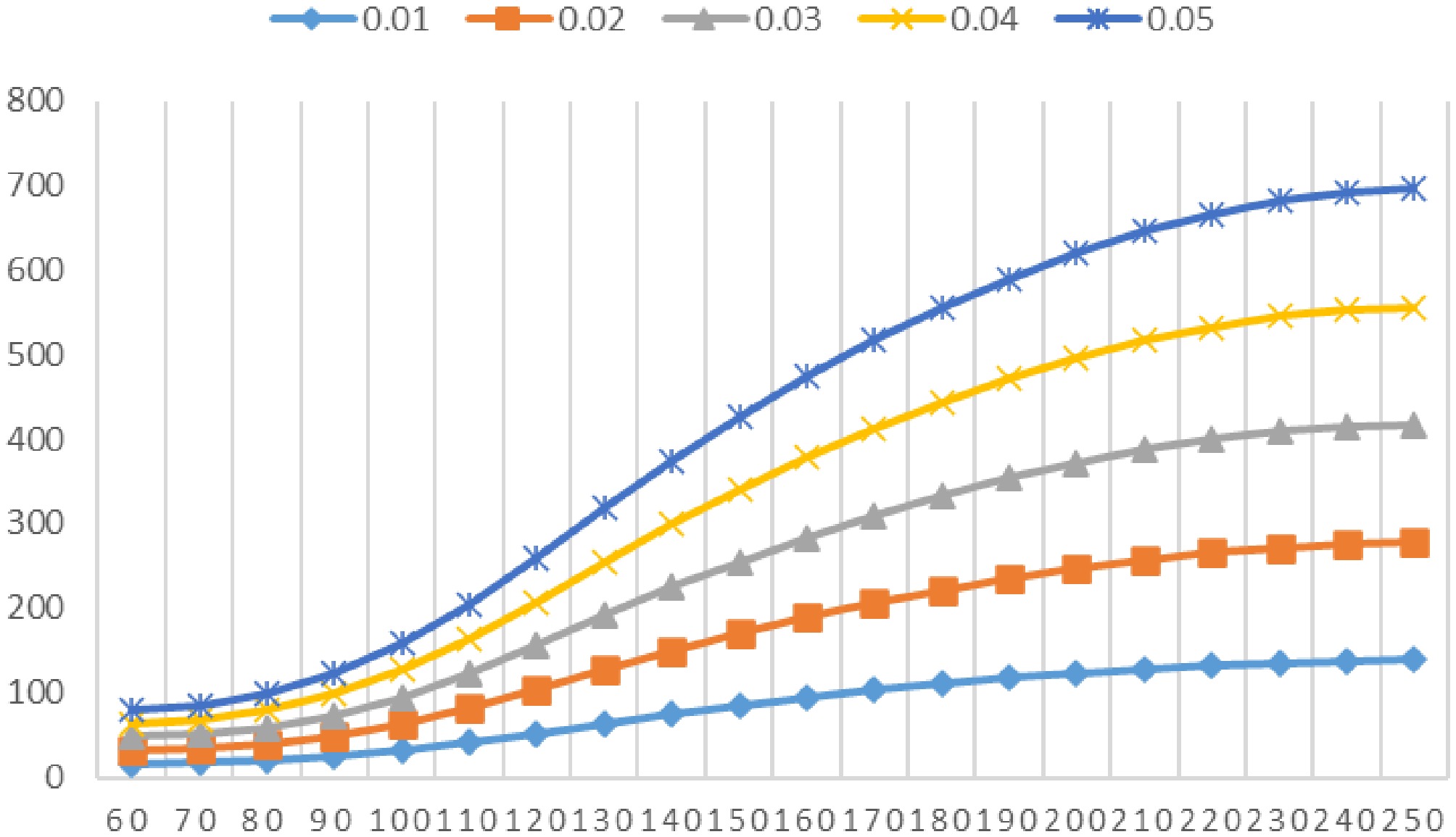
Figure 9.
Impact of asset growth rate (a) on the number of damaged assets across various storm severities.
Assets depreciate over time, characterized by the annual failure rate (λ). As expected, a higher failure rate reduces the number of assets surviving to older ages, thereby altering the lifetime distribution. Table 7 and Fig. 10 demonstrate that for a given total asset count, a higher failure rate shifts the population towards newer assets, indirectly reducing the inventory's average age.
Table 7. Sensitivity analysis: Asset count by lifetime for different failure rates (λ) from 0.01 to 0.05.
Number of assets in
each lifetimeλ 0.01 % 0.02 % 0.03 % 0.04 % 0.05 % 1 1,000 1 1,000 1 1,000 1 1,000 1 1,000 1 2 961.165 0.961165 951.456 0.951456 941.748 0.941748 932.039 0.932039 922.33 0.92233 3 923.838 0.923838 905.269 0.905269 886.889 0.886889 868.696 0.868696 850.693 0.85069 4 887.961 0.887961 861.324 0.861324 835.225 0.835225 809.659 0.809659 784.62 0.78462 5 853.477 0.853477 819.512 0.819512 786.571 0.786571 754.633 0.754633 723.678 0.72368 6 820.332 0.820332 779.73 0.77973 740.752 0.740752 703.348 0.703348 667.47 0.66747 7 788.475 0.788475 741.879 0.741879 697.601 0.697601 655.547 0.655547 615.628 0.61563 8 757.854 0.757854 705.866 0.705866 656.964 0.656964 610.996 0.610996 567.812 0.56781 9 728.423 0.728423 671.6 0.6716 618.694 0.618694 569.472 0.569472 523.71 0.52371 10 700.135 0.700135 638.998 0.638998 582.654 0.582654 530.77 0.53077 483.034 0.48303 11 672.945 0.672945 607.979 0.607979 548.713 0.548713 494.698 0.494698 445.517 0.44552 12 646.811 0.646811 578.465 0.578465 516.749 0.516749 461.078 0.461078 410.913 0.41091 13 621.693 0.621693 550.385 0.550385 486.647 0.486647 429.742 0.429742 378.998 0.379 14 597.549 0.597549 523.667 0.523667 458.299 0.458299 400.537 0.400537 349.561 0.34956 15 574.343 0.574343 498.246 0.498246 431.602 0.431602 373.316 0.373316 322.411 0.32241 16 552.039 0.552039 474.059 0.474059 406.46 0.40646 347.945 0.347945 297.369 0.29737 17 530.6 0.5306 451.047 0.451047 382.783 0.382783 324.298 0.324298 274.272 0.27427 18 509.995 0.509995 429.151 0.429151 360.485 0.360485 302.258 0.302258 252.97 0.25297 19 490.189 0.490189 408.319 0.408319 339.486 0.339486 281.716 0.281716 233.322 0.23332 20 471.152 0.471152 388.497 0.388497 319.71 0.31971 262.571 0.262571 215.2 0.2152 21 452.855 0.452855 369.638 0.369638 301.086 0.301086 244.726 0.244726 198.485 0.19849 22 435.269 0.435269 351.695 0.351695 283.547 0.283547 228.094 0.228094 183.069 0.18307 23 418.365 0.418365 334.622 0.334622 267.03 0.26703 212.593 0.212593 168.85 0.16885 24 402.118 0.402118 318.378 0.318378 251.474 0.251474 198.145 0.198145 155.735 0.15574 25 386.502 0.386502 302.923 0.302923 236.825 0.236825 184.678 0.184678 143.639 0.14364 26 371.492 0.371492 288.218 0.288218 223.03 0.22303 172.128 0.172128 132.483 0.13248 27 357.065 0.357065 274.227 0.274227 210.038 0.210038 160.43 0.16043 122.193 0.12219 28 343.198 0.343198 260.915 0.260915 197.803 0.197803 149.527 0.149527 112.702 0.1127 29 329.87 0.32987 248.249 0.248249 186.28 0.18628 139.365 0.139365 103.949 0.10395 30 317.06 0.31706 236.198 0.236198 175.429 0.175429 129.893 0.129893 95.8749 0.09587 17,902.8 17.90277 15,970.5 15.97051 14,330.6 14.33057 12,932.9 12.93289 11,736.5 11.7365 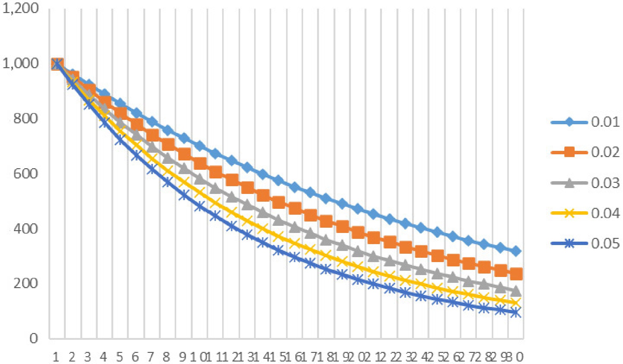
Figure 10.
Sensitivity of asset lifetime distribution to variations in the annual failure rate (λ).
The analysis underscores the critical role of asset 'immunization'. For an even with a given intensity, such as a storm with 105 km/h winds, older assets account for a disproportionately high share of total failures (see Fig. 11). Therefore, investing in strengthening or 'immunizing' older assets is a highly effective strategy. This proactive approach reduces the number of assets that would otherwise fail, thereby decreasing the required inventory for the crisis warehouse and flattening the demand curve for spares.
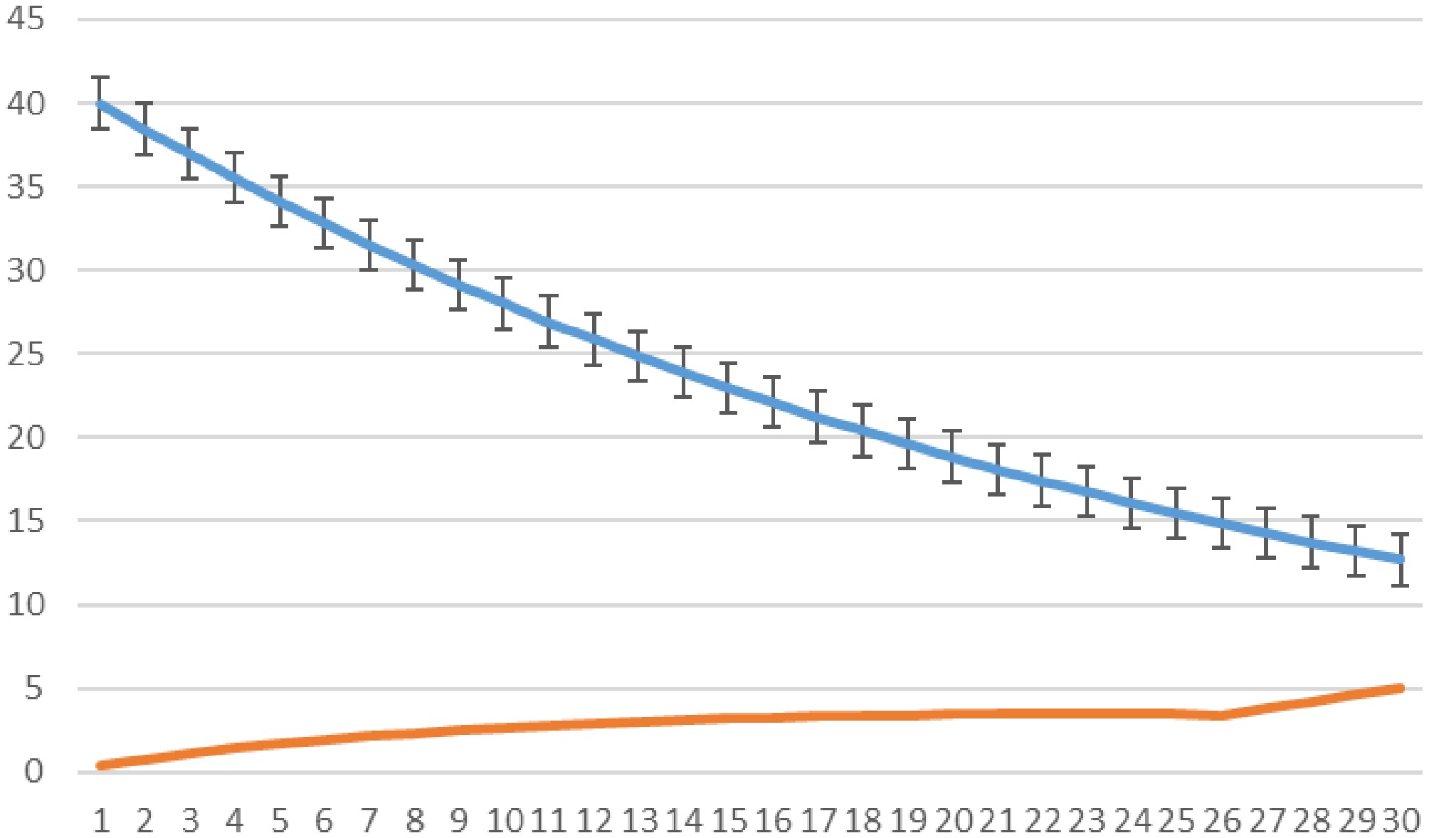
Figure 11.
Distribution of available vs. damaged assets by lifetime at a specific storm severity (105 km/h).
The model's projection over a five-year horizon (Table 8 and Fig. 12) confirms that with a constant asset growth rate, the absolute number of damaged assets for a given event severity will also increase. This is a direct consequence of a larger asset base, assuming that the failure rate (λ) remains constant. The key insight is that the required size of the crisis warehouse must scale proportionally with the growth of the total asset inventory to maintain a constant level of resilience.
Table 8. Projection of potential failures over 5 years at a storm severity of 110 km/h and a 3% asset growth rate.
SeverityTotal number of assets 20,000 20,600 21,218 21,854.5 22,510.2 60 80.2 82.606 85.0842 87.6367 90.2658 70 84.37 86.9011 89.5081 92.1934 94.9592 80 98.72 101.682 104.732 107.874 111.11 90 123.29 126.989 130.798 134.722 138.764 100 158.64 163.399 168.301 173.35 178.551 110 204.67 210.81 217.134 223.648 230.358 120 259.6 267.388 275.41 283.672 292.182 130 319.03 328.601 338.459 348.613 359.071 140 374.43 385.663 397.233 409.15 421.424 150 425.79 438.564 451.721 465.272 479.23 160 473.07 487.262 501.88 516.936 532.445 170 516.22 531.707 547.658 564.088 581.01 180 555.12 571.774 588.927 606.595 624.793 190 589.65 607.34 625.56 644.327 663.656 200 619.68 638.27 657.419 677.141 697.455 210 645.02 664.371 684.302 704.831 725.976 220 665.48 685.444 706.008 727.188 749.004 230 680.84 701.265 722.303 743.972 766.291 240 690.86 711.586 732.933 754.921 777.569 250 695.25 716.108 737.591 759.718 782.51 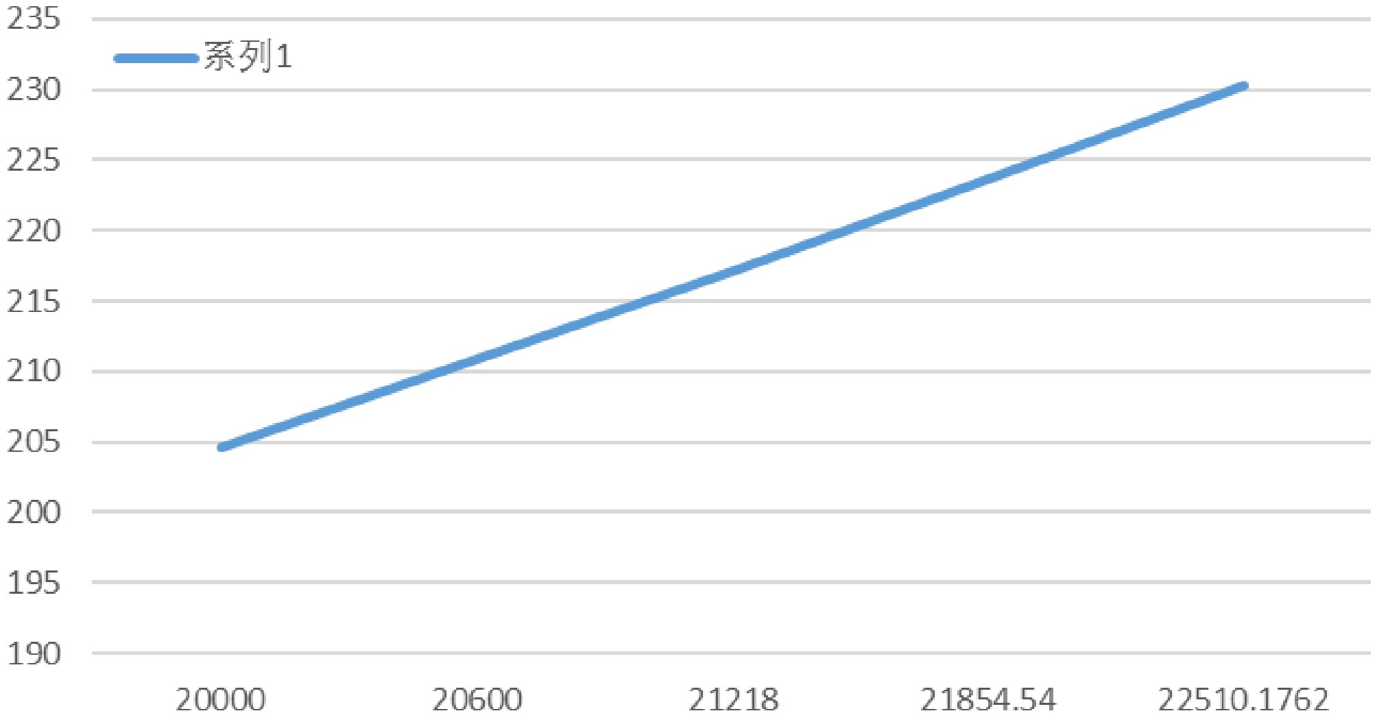
Figure 12.
Projection of potential asset failures over five consecutive years at a storm severity of 110 km/h, assuming a 3% annual asset growth rate.
The sensitivity analysis highlights the importance of asset 'immunization' or targeted reinforcement of older infrastructure. Figure 11 confirms that older assets account for a disproportionately high share of total failures. Investing in strengthening these assets effectively raises their fragility thresholds, which flattens the demand curve for spare parts during crises and reduces the required crisis warehouse inventory.
The model's applicability and limitations
-
Although the proposed framework offers a robust tool for quantifying emergency resource requirements, certain limitations must be acknowledged. First, the model utilizes a linear fragility function (Eq. 1) for computational simplicity. Although validated by the TREDC dataset, nonlinear fragility curves may provide higher precision for specific equipment types or different hazard profiles. Second, the model assumes that the annual failure rate and load growth rate remain constant over the projection horizon. In reality, these parameters can fluctuate because of economic factors or policy changes; thus, the model's projections serve as estimates rather than deterministic predictions. Third, the current framework quantifies the total number of required spares but does not explicitly optimize the spatial distribution of warehouses across the grid, a critical factor for reducing the restoration time. Future work should incorporate geographic information system (GIS) data to optimize the location-based allocation of the crisis inventory alongside the quantity.
-
This paper presents a data-driven decision-support framework for emergency resource management in power distribution networks. By statistically calibrating engineering fragility curves with a decade of operational data from TREDC, we transformed the qualitative process of crisis warehousing into a quantitative, scientifically grounded practice. The results demonstrate that spare asset requirements are highly sensitive to storms' severity, assets' age distribution, and the network's growth rates. Specifically, we clarified that although network growth improves the average age of assets, it increases the absolute number of assets at risk, requiring larger emergency inventories. This framework provides utility managers with a powerful tool to optimize resource allocation, ensuring that resilience planning keeps pace with infrastructure expansion and climate challenges. Future research will focus on integrating an optimization layer to minimize the total cost (inventory holding cost + shortage penalty) and exploring the impact of decentralized generation and mobile emergency units on reducing dependence on warehouses.
This work was supported by the Iran University of Science and Technology. We acknowledge TREDC for providing the operational data used in this study.
-
The authors confirm their contribution to the paper as follows: Validation, resources, methodology, software, formal analysis, investigation, writing – original draft: Yousefi Jooben A; conceptualization, supervision, writing – review and editing: Dashti R. All authors reviewed the results and approved the final version of the manuscript.
-
The datasets generated during and/or analyzed in the current study are available from the corresponding author on reasonable request. The data are not publicly available because of privacy/ethical restrictions associated with the operational records of TREDC.
-
The authors declare that they have no conflict of interest.
- Copyright: © 2026 by the author(s). Published by Maximum Academic Press on behalf of Nanjing Tech University. This article is an open access article distributed under Creative Commons Attribution License (CC BY 4.0), visit https://creativecommons.org/licenses/by/4.0/.
-
About this article
Cite this article
Yousefi Joobeni A, Dashti R. 2026. A data-driven decision support framework for emergency resource management in critical infrastructure. Emergency Management Science and Technology 6: e005 doi: 10.48130/emst-0026-0005 

A data-driven decision support framework for emergency resource management in critical infrastructure
- Received: 13 December 2025
- Revised: 19 February 2026
- Accepted: 16 March 2026
- Published online: 25 May 2026
Abstract: Effective emergency management of critical infrastructure following high-impact–low-probability events is a significant scientific and technological challenge. A critical failure point is often the lack of pre-positioned spare assets, which cripples recovery efforts. This paper proposes a data-driven decision-support framework to enhance emergency logistics and resource allocation. By integrating engineering fragility curves with a unique 10-year operational dataset, our model quantifies the precise number of asset failures required to ensure the rapid restoration of services. Specifically, we utilize historical failure records and meteorological data to calibrate asset fragility curves, moving beyond qualitative assessments. This framework enables emergency managers to shift from heuristic risk assessments to a data-driven budgeting process, quantifying inventory requirements to balance costs against the socioeconomic impact of prolonged disruptions. Our results provide a powerful scientific tool for enhancing the resilience and recovery capabilities of critical infrastructure systems.