













-
Identification of gene–environment (G × E) interactions has long been a central focus in genetic epidemiology. G × E interactions cause variation in the effect of a genotype on disease risk across different environmental exposure conditions[1,2]. Traditionally, G × E interactions have been studied using models that consider a single environmental exposure, with subsequent extensions allowing for nonlinear G × E effects[3]. However, an increasing number of epidemiological studies suggest that disease risk may be influenced by simultaneous exposure to multiple environmental factors[4,5]. When both multiple genetic and environmental variables are incorporated, the model dimension increases substantially due to the inclusion of numerous interaction terms, leading to estimation instability and inflated standard errors, a phenomenon commonly referred to as the curse of dimensionality. To alleviate this burden, the varying multi-index coefficient model (VMICM) proposed by Liu et al.[6] has been applied to model the interaction between a mixture of environmental variables
$ {\boldsymbol{X}} $ $ {\boldsymbol{G}} $ $ {\boldsymbol{Y}} = \sum\limits_{k = 0}^p m_k( {\boldsymbol{X}} {\boldsymbol{\beta}} ) G_k + {\boldsymbol{\epsilon}}, $ (1) where
$ m_k(\cdot) $ $ k = 0,1,\cdots,p $ $ {\boldsymbol{\beta}} $ $ q $ $ q $ $ {\boldsymbol{\epsilon}} $ $ p $ $ q $ $ m_k(\cdot) $ Model (1) is developed for continuous traits, where the primary objective is to model the conditional mean effect. For a binary trait, Guan et al.[8] extended model (1) and proposed a variable selection framework to identify important genetic and environmental variables. In practical applications, however, researchers are often interested in assessing genetic effects at specific quantiles of a continuous trait distribution rather than at the mean. For example, in studies on birth weight, the focus is typically not on how genes influence the average birth weight, but rather on the upper or lower quantiles of the distribution, since extremely high or low birth weight may lead to long-term health complications[9,10]. Even when interest lies in the central tendency of the conditional distribution, median regression (quantile regression with
$ \tau $ With the widespread availability of hundreds of thousands, or even millions, of single-nucleotide polymorphisms (SNPs), genetic studies now operate in inherently high-dimensional settings. In such contexts, traditional model selection procedures, including forward or backward stepwise selection and information-criterion-based approaches such as AIC or Bayesian information criterion (BIC), become computationally impractical and statistically unreliable. When the number of predictors is large relative to the sample size, classical selection methods often exhibit instability, inflated variance, and poor reproducibility. To overcome these limitations, penalized regression methods have become a powerful and widely adopted framework for high-dimensional variable selection. The key idea is to augment the loss (or likelihood) function with a penalty term, thereby enabling simultaneous parameter estimation and variable selection. Different penalty functions yield estimators with distinct theoretical and practical properties, such as sparsity, reduced estimation bias, and computational scalability, making penalized approaches particularly well suited for large-scale genetic analyses. Fan & Li[11] established three desirable properties for penalized estimators: sparsity, unbiasedness, and continuity. They further introduced the concept of the oracle property, according to which an estimator performs asymptotically as well as if the true underlying model were known in advance. Since then, a rich class of penalization methods has been developed. For example, the smoothly clipped absolute deviation (SCAD) penalty[11] and the minimax concave penalty (MCP)[12] are nonconvex penalties designed to reduce estimation bias while maintaining sparsity. The adaptive LASSO[13] method achieves the oracle property through data-driven weights applied to the
$ \ell_1 $ Building upon this rich body of literature, we propose a quantile regression-based variable selection framework under model (1) to investigate how the modification of genetic effects by simultaneous exposure to multiple environmental factors influences a disease trait under different quantiles. The proposed approach incorporates the MCP penalty within a high-dimensional penalized quantile regression framework to achieve effective variable selection while reducing the estimation bias. We assess the performance of the proposed method through comprehensive simulation studies and real-data analysis. By extending penalized variable selection techniques to the quantile varying multi-index coefficient model, our work contributes to and enriches the existing literature on high-dimensional variable selection for quantile regression.
Although the proposed framework is motivated by existing varying multi-index coefficient models for mean and binary outcomes, extending these approaches to a high-dimensional quantile regression setting leads to substantial additional challenges due to the non-smooth quantile loss function, nonconvex penalization, spline approximation, and iterative optimization procedure. The primary objective of the current work is therefore to develop a practical estimation and variable selection framework together with empirical evaluation through simulations and real-data analysis. A formal theoretical investigation of identifiability, estimation consistency, oracle properties, and convergence behavior under the proposed quantile framework remains an important topic for future research. The rest of the paper is organized as follows. The following section introduces the proposed variable selection framework, including the penalized quantile loss function, the iterative estimation algorithm, and the selection of tuning parameters and initial values for
$ {\boldsymbol{\beta}} $ -
Throughout the paper, superscript
$ T $ $ \|\cdot\|_p $ $ L_p $ $ a $ Model setup
-
For a random sample of size
$ n $ $ {\boldsymbol{Y}}_{n\times 1} $ $ {\boldsymbol{X}}_{n\times q} $ $ {\boldsymbol{G}}_{n\times (p+1)} $ $ {\boldsymbol{Y}}(\tau) = \sum\limits_{k = 0}^p m_k( {\boldsymbol{X}} {\boldsymbol{\beta}}(\tau),\tau) {\boldsymbol{G}}_k + {\boldsymbol{\epsilon}}(\tau), $ (2) where
$ {\boldsymbol{Y}} = (Y_1, Y_2,\cdots, Y_n)^T $ $ {\boldsymbol{X}} = ( {\boldsymbol{X}}_1, {\boldsymbol{X}}_2, \cdots, {\boldsymbol{X}}_q) $ $ q $ $ {\boldsymbol{G}}_{n\times(p+1)} = ( {\boldsymbol{G}}_0, {\boldsymbol{G}}_1, \cdots, {\boldsymbol{G}}_p) $ $ {\boldsymbol{G}}_0 = (1,\cdots,1)^T $ $ {\boldsymbol{G}}_k $ $ n $ $ k $ $ k = 1,2,\cdots,p $ $ \{m_k(\cdot,\tau)\}_{k=0,1,\cdots,p} $ $ \tau $ $ {\boldsymbol{\beta}}(\tau) = (\beta_1(\tau),\cdots,\beta_q(\tau))^T $ $ {\boldsymbol{\epsilon}}(\tau) $ $ P\{ {\boldsymbol{\epsilon}}(\tau)<0 \mid {\boldsymbol{X}}, {\boldsymbol{G}}\} = \tau $ $ 0<\tau<1 $ $ \tau=0.5 $ $ {\boldsymbol{\beta}} $ $ m_k(\cdot) $ $ {\boldsymbol{\beta}}(\tau) $ $ m_k(\cdot,\tau) $ Parameter estimation
-
Our goal is to estimate and select unknown functions
$ \{m_k(\cdot)\}_{k = 0, 1, \cdots, p} $ $ {\boldsymbol{\beta}} = (\beta_1, \cdots, \beta_q)^T $ $ \| {\boldsymbol{\beta}}\|_2 = 1 $ $ \beta_{1} \gt 0 $ $ m_k(\cdot) $ $ m_k( {\boldsymbol{u}}) = {\boldsymbol{\alpha}}^T {\boldsymbol{u}} {\boldsymbol{\beta}}^T {\boldsymbol{u}} + {\boldsymbol{\gamma}}^T {\boldsymbol{u}} + c $ $ m_k(\cdot) $ $ u= {\boldsymbol{X}} {\boldsymbol{\beta}} $ $ m_k(\cdot) $ $ K $ $ h $ $ m_k(u) \approx \gamma_{k1} + \bar{ {\boldsymbol{B}}}(u) {\boldsymbol{\gamma}}_{k*}, $ (3) where
$ \bar{ {\boldsymbol{B}}}(u) $ $ {\boldsymbol{\gamma}}_{k*}=(\gamma_{k2},\gamma_{k3},\cdots,\gamma_{kL})^T $ $ {\boldsymbol{\gamma}}_k=(\gamma_{k1}, {\boldsymbol{\gamma}}_{k*}^T)^T $ $ L=K+h+1 $ $ {\boldsymbol{Y}} = \sum\limits_{k=0}^p \left\{\gamma_{k1}+\bar{ {\boldsymbol{B}}}( {\boldsymbol{X}} {\boldsymbol{\beta}}) {\boldsymbol{\gamma}}_{k*}\right\} {\boldsymbol{G}}_k+ {\boldsymbol{\epsilon}}. $ (4) Thus, estimating the unknown functions
$ \{m_k(\cdot)\}_{k=0}^p $ $ \{\gamma_{k1}, {\boldsymbol{\gamma}}_{k*}\}_{k=0}^p $ $ {\boldsymbol{\beta}} $ $ \| {\boldsymbol{\gamma}}_{k*}\|_2\neq 0 $ $ {\boldsymbol{G}}_k $ $ {\boldsymbol{X}} {\boldsymbol{\beta}} $ $ \| {\boldsymbol{\gamma}}_{k*}\|_2=0 $ $ |\gamma_{k1}|\neq 0 $ $ {\boldsymbol{G}}_k $ $ \| {\boldsymbol{\gamma}}_{k*}\|_2=0 $ $ |\gamma_{k1}|=0 $ $ {\boldsymbol{G}}_k $ $ {\boldsymbol{Y}} $ Motivated by Guan et al.[7], we estimate the model parameters by minimizing the penalized quantile loss. Let
$ \rho_{\tau}(u)=u\{\tau-I(u<0)\} $ $ \begin{split} Q_{\tau}( {\boldsymbol{\beta}}, {\boldsymbol{\gamma}}) =& \sum\limits_{i=1}^n \rho_{\tau}\left(Y_i-\sum\limits_{k=0}^p \left\{\gamma_{k1}+\bar{ {\boldsymbol{B}}}( {\boldsymbol{X}} {\boldsymbol{\beta}}) {\boldsymbol{\gamma}}_{k*}\right\}G_{ik}\right) \\ & + n\sum\limits_{k=1}^p p_{\lambda_1}(\| {\boldsymbol{\gamma}}_{k*}\|_2) + n\sum\limits_{k=1}^p p_{\lambda_2}(|\gamma_{k1}|)I(\| {\boldsymbol{\gamma}}_{k*}\|_2=0) + n\sum\limits_{d=2}^q p_{\lambda_3}(|\beta_d|). \end{split} $ (5) The first term measures the lack of fit under quantile regression, while the remaining terms impose sparsity on the varying components, constant genetic effects, and environmental loading parameters, respectively. The penalty
$ p_{\lambda_1}(\cdot) $ $ \| {\boldsymbol{\gamma}}_{k*}\|_2 $ $ k $ $ p_{\lambda_2}(\cdot) $ $ \gamma_{k1} $ $ p_{\lambda_3}(\cdot) $ $ {\boldsymbol{\beta}} $ $ m_0(\cdot) $ $ {\boldsymbol{\gamma}}_{0*} $ $ \gamma_{01} $ $ \beta_1 $ $ \beta_1>0 $ $ p(x,\lambda)=\lambda\int_0^x\left(1-\dfrac{s}{\delta\lambda}\right)_+\mathrm{d}s, $ where
$ \lambda>0 $ $ \delta>0 $ Estimation algorithm
-
Guan et al.[7,8] developed three-step iterative procedures for Model (1) in the conditional mean and binary response settings. These procedures classify each nonparametric function
$ m_k(\cdot) $ Step 1: For a given
$ {\boldsymbol{\beta}} $ $ \hat{ {\boldsymbol{\beta}}}^{(0)} $ $ {\boldsymbol{\gamma}} $ $ \hat{ {\boldsymbol{\gamma}}}^{(1)} = \{ \hat{\gamma}_{k1}^{(1)}, \hat{ {\boldsymbol{\gamma}}}_{k*}^{(1)T}\}^T_{k = 0,1,\cdots,p} $ $ \hat{\boldsymbol{\gamma}}^{(1)}=\min\limits_{\boldsymbol{\gamma}}Q_1(\boldsymbol{\gamma}|\lambda_1,\hat{\boldsymbol{\beta}}^{(0)}), $ where
$ Q_1( {\boldsymbol{\gamma}}|\lambda_1, \hat{ {\boldsymbol{\beta}}}^{(0)}) = \sum\limits_{i=1}^n \rho_{\tau}\left(Y_i -\sum\limits_{k =0}^p [\gamma_{k1} + \bar{ {\boldsymbol{B}}}( {\boldsymbol{X}} {\boldsymbol{\beta}}^{(0)}) {\boldsymbol{\gamma}}_{k*}]G_{ik} \right)+ n\sum\limits_{k=1}^p p_{\lambda_1}(\| {\boldsymbol{\gamma}}_{k*}\|_2). $ Rather than penalizing the individual components of
$ {\boldsymbol{\gamma}}_{k*} = (\gamma_{k2},\cdots,\gamma_{kL})^T $ $ L_2 $ $ {\boldsymbol{G}}_k $ $ {\boldsymbol{\gamma}}_{k*} $ $ m_k(\cdot) $ $ k=1,\cdots,p $ $ m_k(\cdot) $ $ \| \hat{ {\boldsymbol{\gamma}}}_{k*}^{(1)}\|_2 \gt 0 $ $ \| \hat{ {\boldsymbol{\gamma}}}_{k*}^{(1)}\|_2 = 0 $ Step 2: Based on the step 1 estimators of the B-spline coefficients
$ {\boldsymbol{\gamma}} $ $ \hat{ {\boldsymbol{\gamma}}}^{(2)} = \{( \hat{\gamma}_{k1}^{(2)}, \hat{ {\boldsymbol{\gamma}}}_{k*}^{(2)})_{k\in V},( \hat{\gamma}_{k1}^{(2)})_{k\in C}\} $ $ \hat{ {\boldsymbol{\gamma}}}_{k*}^{(2)} = 0 $ $ \hat{ {\boldsymbol{\gamma}}}_{k*}^{(1)} = 0 $ $ \hat{ {\boldsymbol{\gamma}}}^{(2)} = \min\limits_{ {\boldsymbol{\gamma}}}Q_2( {\boldsymbol{\gamma}}|\lambda_2, {\boldsymbol{\beta}}^{(0)}, \hat{ {\boldsymbol{\gamma}}}^{(1)}) $ where
$ \begin{split} Q_2\left( {\boldsymbol{\gamma}}|\lambda_2, {\boldsymbol{\beta}}^{(0)}, \hat{ {\boldsymbol{\gamma}}}^{(1)}\right) = &\sum\limits_{i=1}^n \rho_{\tau}\left(Y_i -\sum\limits_{k\in V} [\gamma_{k1} + \bar{ {\boldsymbol{B}}}( {\boldsymbol{X}} {\boldsymbol{\beta}}^{(0)}) {\boldsymbol{\gamma}}_{k*}]G_{ik} -\sum\limits_{k\in C}\gamma_{k1}^{(2)}G_{ik} \right)\\ & + n\sum\limits_{k=1}^p p_{\lambda_2}(|\gamma_{k1}^{(2)}|)I(\| \hat{ {\boldsymbol{\gamma}}}_{k*}^{(1)}\|_2 = 0).\end{split}$ (6) Based on the initial estimator of
$ {\boldsymbol{\beta}} $ $ \hat{ {\boldsymbol{\beta}}}^{(0)} $ $ {\boldsymbol{\gamma}} $ $ \hat{ {\boldsymbol{\gamma}}}^{(2)} $ $ m_k(\cdot), \ k= 1,\cdots,p $ Step 3: Update
$ \hat{ {\boldsymbol{\beta}}} $ $ \hat{ {\boldsymbol{\beta}}} = \min\limits_{\| {\boldsymbol{\beta}}\|_2=1}Q_3( {\boldsymbol{\beta}}|\lambda_3, \hat{ {\boldsymbol{\gamma}}}^{(2)}), $ where
$ Q_3( {\boldsymbol{\beta}}|\lambda_3, \hat{ {\boldsymbol{\gamma}}}^{(2)}) = \sum\limits_{i=1}^n \rho_{\tau}\left(Y_i -\sum\limits_{k =0}^p [ \hat{\gamma}_{k1}^{(2)} + \bar{ {\boldsymbol{B}}}( {\boldsymbol{X}} {\boldsymbol{\beta}}) \hat{ {\boldsymbol{\gamma}}}_{k*}^{(2)}]G_{ik} \right) + n\sum\limits_{d=2}^{q} p_{\lambda_3}(|\beta_d|). $ Step 4: Set
$ \hat{ {\boldsymbol{\beta}}}^{(0)} = \hat{ {\boldsymbol{\beta}}} $ $ \hat{ {\boldsymbol{\gamma}}} $ $ \hat{ {\boldsymbol{\beta}}} $ $ \dfrac{\| \hat{\beta}^{(t+1)} - \hat{\beta}^{(t)}\|_2}{\| \hat{\beta}^{(t)}\|_2} \lt 10^{-4} $ Due to the discontinuous penalty structure involving the indicator function
$ I(\|\gamma_{k*}\|_2 = 0) $ From a computational perspective, the main cost of the proposed procedure arises from repeated penalized quantile regression fitting during the grid search for the tuning parameters
$ \lambda_1 $ $ \lambda_2 $ $ \lambda_3 $ $ h $ $ K $ Additional details on the estimation algorithm are provided in the Supplementary File 1. The implementation of the iterative procedure requires selecting the tuning parameters
$ \lambda_1 $ $ \lambda_2 $ $ \lambda_3 $ $ h $ $ K $ $ {\boldsymbol{\beta}} $ Selection of parameters
-
The BIC[21] is widely used for tuning parameter selection in linear mean regression models. Its use in quantile regression has also been theoretically justified[22,23]. Accordingly, we use a BIC-type criterion to select the tuning parameters, together with the spline degree
$ h $ $ K $ Selection of the tuning parameters $ {\boldsymbol{\lambda}}_1, {\boldsymbol{\lambda}}_2, {\boldsymbol{\lambda}}_3 $
-
Step 1: We select
$ \lambda_1 $ $ \mathrm{BIC}(\lambda_1) = \log \left\{ \sum\limits_{i=1}^n \rho_{\tau}\left(Y_i - \sum\limits_{k=0}^p \left[ \hat{\gamma}_{k1}^{(\lambda_1)} + \bar{ {\boldsymbol{B}}}( {\boldsymbol{X}} \hat{ {\boldsymbol{\beta}}}^{(0)}) \hat{ {\boldsymbol{\gamma}}}_{k*}^{(\lambda_1)} \right] G_{ik} \right) \right\} + \dfrac{\log(n)}{2n} \, df_{\lambda_1}, $ where
$ \{ \hat{\gamma}_{k1}^{(\lambda_1)}, \hat{ {\boldsymbol{\gamma}}}_{k*}^{(\lambda_1)}\}_{k=0,1,\cdots,p} $ $ Q_1( {\boldsymbol{\gamma}} \mid \lambda_1, \hat{ {\boldsymbol{\beta}}}^{(0)}) $ $ \hat{ {\boldsymbol{\beta}}}^{(0)} $ $ df_{\lambda_1} $ $ \lambda_1 $ Step 2: We select
$ \lambda_2 $ $ \mathrm{BIC}(\lambda_2) = \log \left\{ \sum\limits_{i=1}^n \rho_{\tau}\left(Y_i - \sum\limits_{k=0}^p \left[ \hat{\gamma}_{k1}^{(\lambda_2)} + \bar{ {\boldsymbol{B}}}( {\boldsymbol{X}} \hat{ {\boldsymbol{\beta}}}^{(0)}) \hat{ {\boldsymbol{\gamma}}}_{k*}^{(\lambda_2)} \right] G_{ik} \right) \right\} + \dfrac{\log(n)}{2n} \, df_{\lambda_2}, $ where
$ \{ \hat{\gamma}_{k1}^{(\lambda_2)}, \hat{ {\boldsymbol{\gamma}}}_{k*}^{(\lambda_2)}\}_{k=0,1,\cdots,p} $ $ Q_2( {\boldsymbol{\gamma}} \mid \lambda_2, \hat{ {\boldsymbol{\beta}}}^{(0)}) $ $ df_{\lambda_2} $ $ \lambda_2 $ Step 3: We select
$ \lambda_3 $ $ \mathrm{BIC}(\lambda_3) = \log \left\{ \sum\limits_{i=1}^n \rho_{\tau}\left(Y_i - \sum\limits_{k=0}^p \left[ \hat{\gamma}_{k1}^{(2)} + \bar{ {\boldsymbol{B}}}( {\boldsymbol{X}} \hat{ {\boldsymbol{\beta}}}^{(\lambda_3)}) \hat{ {\boldsymbol{\gamma}}}_{k*}^{(2)} \right] G_{ik} \right) \right\} + \dfrac{\log(n)}{2n} \, df_{\lambda_3}, $ where
$ \hat{ {\boldsymbol{\beta}}}^{(\lambda_3)} $ $ Q_3( {\boldsymbol{\beta}} \mid \lambda_3, \hat{ {\boldsymbol{\gamma}}}^{(2)}) $ $ df_{\lambda_3} $ $ {\boldsymbol{\beta}} $ $ \lambda_3 $ $ \beta $ To determine the optimal tuning parameters,
$ \lambda_1 $ $ \lambda_2 $ $ \lambda_3 $ $ 10^{-3} $ Selection of the order h and the number of interior knots K
-
As discussed in Guan et al.[7], a higher order of the B-spline basis functions allows for greater flexibility but results in more complex functional forms and reduced interpretability. From a practical perspective, G × E effects are unlikely to exhibit highly nonlinear patterns. To balance model flexibility and interpretability, we look for the optimal spline order over the set
$ h \in \{2,3,4\} $ For the number of interior knots
$ K $ $ \mathscr{K} = \{2,3,4,5\} $ $ K $ $ h $ $ Y = m_0( {\boldsymbol{X}} {\boldsymbol{\beta}}) + {\boldsymbol{\epsilon}}. $ (7) As noted in Guan et al.[7], this strategy substantially reduces the computational burden compared to fitting the full model for every
$ (K,h) $ $ K $ $ h $ $ \log \left\{ \sum\limits_{i=1}^n \rho_{\tau}(Y_i - \hat{Y}_i) \right\} + \dfrac{\log(n)}{2n} (K + h + 1), $ where
$ \hat{Y}_i $ $ i $ $ h $ $ K $ $ m_k(\cdot) $ Selection of the initial values
-
For single-index models, the initial value of
$ {\boldsymbol{\beta}} $ $ (1,0,\cdots,0)^T $ $ (1/\sqrt{q},\cdots,1/\sqrt{q})^T $ $ {\boldsymbol{\beta}} $ $ {\boldsymbol{X}} {\boldsymbol{\beta}} $ $ {\boldsymbol{\beta}} $ -
We performed simulation studies to examine the finite-sample performance of the proposed variable selection procedure. Performance was evaluated using four criteria: the oracle percentage for classifying the nonparametric functions
$ m_k(u) $ $ \hat{m}_k(u) $ $ {\boldsymbol{\beta}} $ $ {\boldsymbol{\beta}} $ The oracle percentage for
$ m_k(u) $ $ m_k(u) $ $ m_k(u) $ $ g $ $ m_k(u) $ $ \dfrac{g}{1,000} \times 100{\text{%}} $ The IMSE of
$ m_k(\cdot) $ $ \dfrac{1}{1,000} \sum\limits_{r=1}^{1,000} \left[ \dfrac{1}{100} \sum\limits_{j=1}^{100} \left( \hat{m}_k^{(r)}(u_j) - m_k(u_j) \right)^2 \right], $ where
$ \hat{m}_k^{(r)}(u_j) $ $ m_k(u_j) $ $ r $ $ u_j $ $ j $ $ {\boldsymbol{X}} \hat{ {\boldsymbol{\beta}}}^{(r)} $ $ m_k(\cdot) $ The oracle percentage for
$ {\boldsymbol{\beta}} $ $ \beta_d \neq 0 $ $ g $ $ \beta_d $ $ \dfrac{g}{1,000} \times 100{\text{%}} $ The MSE of
$ \beta_d $ $ \dfrac{1}{1,000} \sum\limits_{r=1}^{1,000} \left( \hat{\beta}_d^{(r)} - \beta_d \right)^2, $ where
$ \hat{\beta}_d^{(r)} $ $ \beta_d $ $ r $ Simulation setting
-
The data were generated according to Model (2). We generated
$ q = 5 $ $ \mathrm{Unif}(0,1) $ $ {\boldsymbol{\beta}} = (\beta_1, \beta_2, \cdots, \beta_q)^T $ $ \beta_1 = \beta_2 = 1/\sqrt{2} $ $ \beta_j = 0 $ $ j = 3,4,5 $ $ {\boldsymbol{\epsilon}} $ $ N(0,1) $ $ \tau $ $ {\boldsymbol{\epsilon}}(\tau) = {\boldsymbol{\epsilon}} - F^{-1}(\tau), $ where
$ F $ $ {\boldsymbol{\epsilon}} $ $ F^{-1}(\tau) $ $ \tau $ $ {\boldsymbol{\epsilon}}(\tau) $ $ {\boldsymbol{G}} $ The continuous case
-
We first evaluated the performance of the proposed method when the genetic predictors
$ {\boldsymbol{G}} $ $ N(0,1) $ $ m_0(u) = 2\sin(2\pi u) $ $ m_1(u) = 2\cos(\pi u) + 2 $ $ m_2(u) = \sin(2\pi u) + \cos(\pi u) + 1 $ $ m_3(u) = 2 $ $ m_4(u) = 2.5 $ $ m_k(u) = 0 $ $ k = 5,\cdots,p $ $ m_0 $ $ m_1 $ $ m_2 $ $ m_3 $ $ m_4 $ $ \tau $ $ n $ Table 1 presents the selection and estimation results for the nonparametric functions
$ m_k(\cdot) $ $ m_0 $ $ m_4 $ $ \tau = 0.5 $ $ \tau = 0.25 $ $ \tau = 0.75 $ Table 1. Selection and estimation accuracy of $ m_k(\cdot) $ for continuous $ {\boldsymbol{G}} $.
$ \tau $ $ m(\cdot) $ p = 50 p = 100 Oracle/% IMSE (Model) IMSE (Oracle) Oracle/% IMSE (Model) IMSE (Oracle) 0.25 $ m_0(.) $ 100.0% 2.78E+00 2.96E−02 100.0% 2.67E+00 2.97E−02 $ m_1(.) $ 100.0% 8.16E−02 6.16E−03 100.0% 7.07E−02 6.16E−03 $ m_2(.) $ 100.0% 9.59E−02 1.30E−02 100.0% 7.80E−02 1.31E−02 $ m_3(.) $ 100.0% 2.58E−02 8.77E−04 100.0% 2.19E−02 9.71E−04 $ m_4(.) $ 100.0% 2.56E−02 1.02E−03 99.8% 2.12E−02 9.80E−04 Zero 88.8% 1.03E−02 0 90.6% 7.27E−03 0 0.5 $ m_0(.) $ 100.0% 7.49E−02 2.88E−02 100.0% 7.70E−02 2.91E−02 $ m_1(.) $ 100.0% 4.98E−02 5.07E−03 100.0% 4.89E−02 5.31E−03 $ m_2(.) $ 100.0% 5.72E−02 1.22E−02 100.0% 5.77E−02 1.23E−02 $ m_3(.) $ 99.7% 1.25E−03 7.90E−04 99.9% 1.30E−03 7.90E−04 $ m_4(.) $ 99.9% 1.50E−03 7.91E−04 99.8% 1.48E−03 8.29E−04 Zero 98.7% 1.00E−04 0 99.1% 6.26E−05 0 0.75 $ m_0(.) $ 100.0% 2.60E+00 3.01E−02 100.0% 2.60E+00 3.13E−02 $ m_1(.) $ 100.0% 6.25E−02 6.08E−03 100.0% 6.17E−02 6.18E−03 $ m_2(.) $ 100.0% 7.12E−02 1.35E−02 100.0% 7.14E−02 1.37E−02 $ m_3(.) $ 99.9% 2.42E−02 8.58E−04 100.0% 2.18E−02 9.03E−04 $ m_4(.) $ 99.9% 2.62E−02 9.93E−04 100.0% 2.20E−02 9.63E−04 Zero 88.5% 1.05E−02 0 90.7% 7.19E−03 0 Regarding estimation accuracy, the IMSE values for
$ m_1 $ $ m_4 $ $ 10^{-2} $ $ 10^{-3} $ $ \tau = 0.5 $ $ \tau = 0.25 $ $ \tau = 0.75 $ $ m_0 $ Table 2 summarizes the selection and estimation results for the loading parameters
$ {\boldsymbol{\beta}} $ $ \beta_1 $ $ \beta_2 $ $ \beta_3 $ $ \beta_4 $ $ \beta_5 $ $ \tau = 0.5 $ $ \tau = 0.25 $ $ \tau = 0.75 $ $ \tau = 0.25 $ $ \tau = 0.75 $ $ p = 50 $ $ p = 100 $ Table 2. Selection and estimation accuracy of $ {\boldsymbol{\beta}} $.
$ \tau $ $ \beta $ p = 50 p = 100 Oracle/% MSE (Model) MSE (Oracle) Oracle/% MSE (Model) MSE (Oracle) 0.25 $ \beta_1 $ 100.0% 1.20E−02 4.76E−05 100.0% 6.71E−03 4.36E−05 $ \beta_2 $ 99.8% 1.47E−02 4.75E−05 100.0% 7.69E−03 4.37E−05 $ \beta_3 $ 99.9% 7.15E−05 0 99.9% 5.81E−05 0 $ \beta_4 $ 99.9% 2.09E−04 0 99.9% 2.93E−04 0 $ \beta_5 $ 99.9% 9.60E−05 0 99.9% 9.53E−05 0 0.5 $ \beta_1 $ 100.0% 5.29E−05 3.78E−05 100.0% 5.33E−05 3.54E−05 $ \beta_2 $ 100.0% 5.29E−05 3.78E−05 100.0% 5.34E−05 3.54E−05 $ \beta_3 $ 98.6% 1.52E−06 0 98.3% 1.23E−06 0 $ \beta_4 $ 98.3% 3.33E−06 0 98.8% 3.24E−06 0 $ \beta_5 $ 98.7% 1.85E−06 0 98.9% 1.45E−06 0 0.75 $ \beta_1 $ 100.0% 4.40E−03 4.81E−05 100.0% 3.60E−03 4.89E−05 $ \beta_2 $ 100.0% 4.51E−03 4.80E−05 100.0% 3.49E−03 4.88E−05 $ \beta_3 $ 95.3% 4.14E−05 0 96.3% 1.87E−05 0 $ \beta_4 $ 95.9% 5.31E−05 0 96.2% 4.23E−05 0 $ \beta_5 $ 95.8% 3.85E−05 0 95.8% 2.32E−05 0 The discrete case
-
We further evaluated the performance of the proposed method with discrete genetic predictors
$ {\boldsymbol{G}} $ $ {\boldsymbol{G}} $ $ P(G_{ij} = 0) = \mathrm{MAF}^2, \; P(G_{ij} = 1) = 2\mathrm{MAF}(1-\mathrm{MAF}), \; P(G_{ij} = 2) = (1-\mathrm{MAF})^2, $ where
$ G_{ij} $ $ j $ $ i $ $ i=1,\cdots,n $ $ j=1,\cdots,p $ $ p=50,100 $ $ \tau=0.25,0.5,0.75 $ $ n=2,000 $ $ m_k(\cdot) $ Table 3. Function $ m_k(\cdot) $ and the corresponding MAF for $ {\boldsymbol{G}}_k $.
$ m(\cdot) $ function MAF of $ {\boldsymbol{G}}_k $ $ m_0(u) = 2sin(2\pi u) $ − $ m_1(u)= 2cos(\pi u) + 2 $ 0.5 $ m_2(u) = sin(2\pi u) + cos(\pi u) + 1 $ 0.5 $ m_3(u)= 2cos(\pi u) + 2 $ 0.3 $ m_4(u) = sin(2\pi u) + cos(\pi u) + 1 $ 0.3 $ m_5(u)= 2cos(\pi u) + 2 $ 0.1 $ m_6(u) = sin(2\pi u) + cos(\pi u) + 1 $ 0.1 $ m_7(u)= 2 $ 0.5 $ m_8(u)= 2 $ 0.3 $ m_9(u)= 2 $ 0.1 $ m_k(u)= 0, k>9 $ Unif (0.05, 0.5) Table 4 summarizes the selection and estimation performance for the nonparametric functions
$ m_k(\cdot) $ $ \tau=0.5 $ $ \tau=0.5 $ $ p=50 $ $ p=100 $ $ \tau=0.5 $ $ \tau=0.25 $ $ \tau=0.75 $ $ p=50 $ $ p=100 $ Table 4. Selection and estimation accuracy for $ m_k(\cdot) $ with discrete $ {\boldsymbol{G}} $.
$ \tau $ Type $ p = 50 $ $ p = 100 $ Oracle/% IMSE (Model) IMSE (Oracle) Oracle/% IMSE (Model) IMSE (Oracle) 0.25 $ m_0(\cdot) $ 100.0% 7.54E−01 2.47E−02 100.0% 7.98E−01 2.44E−02 V 97.5% 1.44E−01 2.30E−02 91.4% 2.23E−01 2.32E−02 C 94.2% 1.66E−02 3.19E−03 95.5% 1.66E−02 3.22E−03 Z 93.9% 4.71E−03 0 96.0% 3.05E−03 0 0.5 $ m_0(\cdot) $ 100.0% 4.84E−02 2.35E−02 100.0% 4.97E−02 2.30E−02 V 99.9% 9.14E−02 2.00E−02 99.3% 9.84E−02 1.98E−02 C 95.4% 7.52E−03 2.68E−03 95.5% 9.30E−03 2.76E−03 Z 93.6% 2.87E−03 0 93.8% 2.87E−03 0 0.75 $ m_0(\cdot) $ 100.0% 1.02E+00 2.53E−02 100.0% 1.09E+00 2.48E−02 V 90.8% 2.29E−01 2.33E−02 84.1% 3.35E−01 2.30E−02 C 96.7% 1.35E−02 3.19E−03 98.6% 1.26E−02 3.14E−03 Z 96.8% 2.09E−03 0 98.5% 9.24E−04 0 Figure 1 further illustrates the relationship between MAF and performance. As MAF increases from 0.1 to 0.5, the oracle percentage increases and the IMSE decreases. This confirms that the model performs better for variants with larger MAF than for those with lower MAF, which is expected because variants with lower MAFs contain less information. This behavior is consistent with the reduced Fisher information for relatively rare variants.
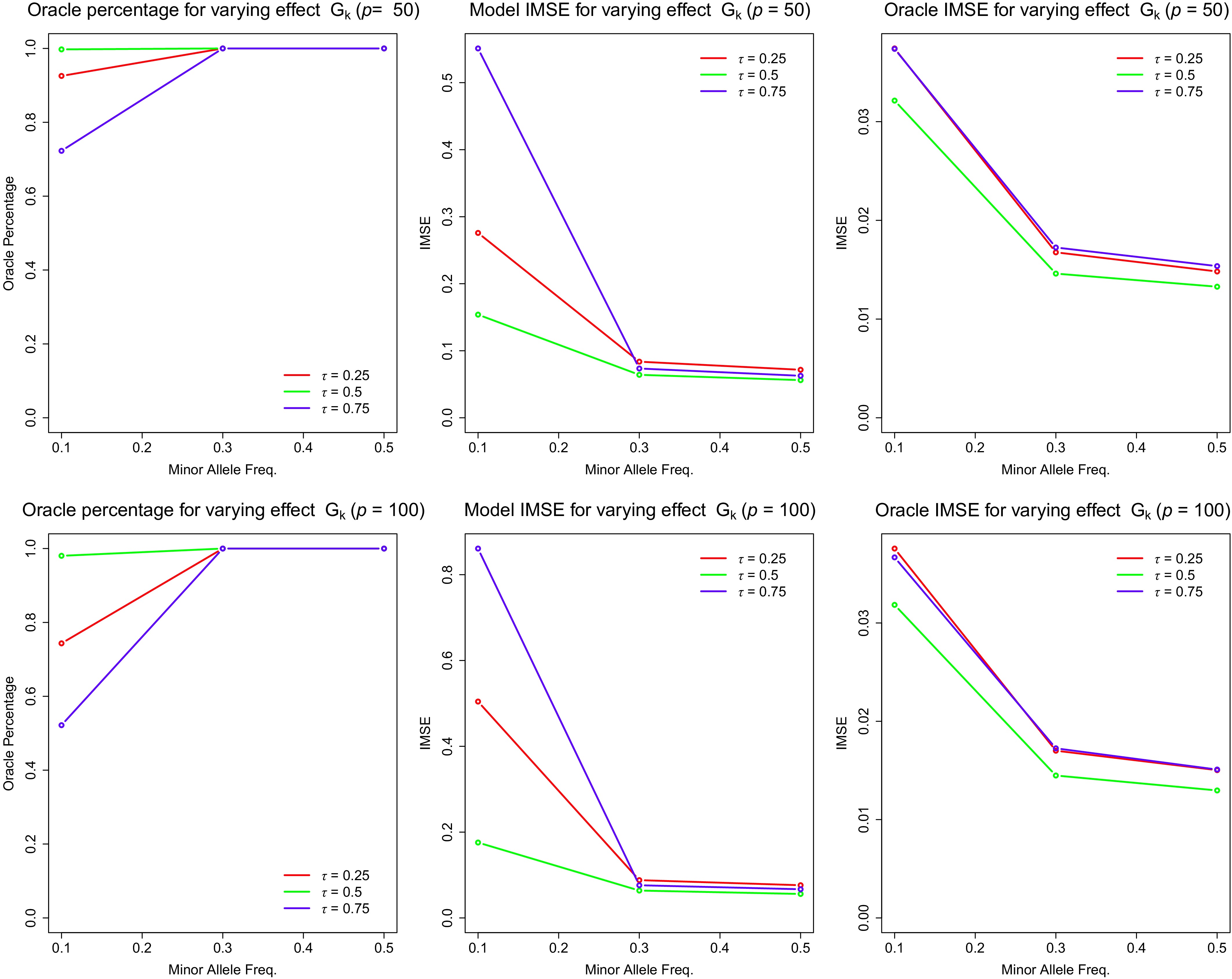
Figure 1.
Selection and estimation accuracy of $ m_k(\cdot) $ for discrete $ {\boldsymbol{G}} $.
Table 5 presents the selection and estimation results for the loading parameters
$ {\boldsymbol{\beta}} $ $ {\boldsymbol{G}} $ $ \beta_1 $ $ \beta_2 $ $ \beta_3,\beta_4,\beta_5 $ $ \tau=0.25 $ $ \tau=0.5 $ $ \tau=0.75 $ $ 10^{-5} $ $ 10^{-7} $ Table 5. Selection and estimation accuracy for $ {\boldsymbol{\beta}} $ with discrete $ {\boldsymbol{G}} $.
$ \tau $ $ \beta $ $ p = 50 $ $ p = 100 $ Oracle/% MSE (Model) MSE (Oracle) Oracle/% MSE (Model) MSE (Oracle) 0.25 $ \beta_1 $ 100.0% 3.98E−04 4.42E−05 100.0% 4.63E−04 4.75E−05 $ \beta_2 $ 100.0% 4.04E−04 4.43E−05 100.0% 4.69E−04 4.74E−05 $ \beta_3 $ 100.0% 0 0 100.0% 0 0 $ \beta_4 $ 100.0% 0 0 100.0% 0 0 $ \beta_5 $ 100.0% 0 0 100.0% 0 0 0.5 $ \beta_1 $ 100.0% 5.20E−05 3.96E−05 100.0% 5.30E−05 3.97E−05 $ \beta_2 $ 100.0% 5.21E−05 3.97E−05 100.0% 5.30E−05 3.97E−05 $ \beta_3 $ 99.1% 2.27E−07 0 99.1% 1.00E−06 0 $ \beta_4 $ 98.9% 3.43E−07 0 98.4% 8.12E−07 0 $ \beta_5 $ 98.9% 5.45E−07 0 98.7% 5.87E−07 0 0.75 $ \beta_1 $ 100.0% 2.75E−04 5.13E−05 100.0% 3.70E−04 4.69E−05 $ \beta_2 $ 100.0% 2.84E−04 5.15E−05 100.0% 3.59E−04 4.69E−05 $ \beta_3 $ 93.6% 2.52E−05 0 93.0% 2.26E−05 0 $ \beta_4 $ 94.3% 2.23E−05 0 93.9% 1.80E−05 0 $ \beta_5 $ 93.5% 3.46E−05 0 93.3% 3.08E−05 0 In summary, the proposed method accurately selects and estimates
$ m(\cdot) $ $ {\boldsymbol{\beta}} $ The current simulation design primarily evaluates the numerical performance of the proposed penalized quantile estimation and variable selection procedure. Specifically, the same true functions
$ m_k(\cdot) $ $ \beta $ $ \tau $ $ m_k(\cdot,\tau) $ $ \beta(\tau) $ Overall, the simulation settings were designed to provide a controlled environment for evaluating whether the proposed method can distinguish varying, constant, and null effect structures. Although some scenarios yielded high selection accuracy, performance decreased in more challenging settings, including tail quantiles, larger model dimensions, and lower MAFs. These patterns are consistent with the increased estimation difficulty in case of more limited information. From a computational perspective, the proposed procedure remains feasible for moderate-scale studies, although repeated penalized quantile regression fitting during tuning parameter selection constitutes the primary computational cost.
-
We applied the proposed variable selection method to a birth-weight data set from the Gene Environment Association Studies initiative (GENEVA), which was supported by the Genes, Environment and Health Initiative (GEI). Birth weight has been widely recognized as an important early-life health indicator, which has established associations with morbidity and mortality during infancy and with risks of multiple diseases later in life[9,10]. Birth weight is influenced by both fetal genetic factors and maternal environmental exposures. After standard quality control procedures, that is, removing SNPs with more than
$ 5{\text{%}} $ $ <0.001 $ For the environmental variables
$ {\boldsymbol{X}} $ $ <0.05 $ $ X_1 $ $ X_2 $ $ X_3 $ All SNPs were mapped to known genes based on genomic location. We retained genes containing at least 30 SNPs, resulting in 2,076 genes for analysis. The proposed model was fitted to each gene at
$ \tau$ $ {\boldsymbol{\beta}} $ The proposed model identified 122 genes with constant genetic effects and no genes with varying effects, suggesting limited evidence of nonlinear G × E interaction with the selected environmental factors in this data set. Given the large number of genes analyzed and the absence of formal multiple-testing adjustment, these findings should be interpreted as exploratory rather than confirmatory. Nevertheless, the absence of varying effects suggests limited evidence of G × E interaction with the selected environmental factors in this data set. As an illustration, we focus on gene ST3GAL1[24], located on chromosome 8, which contains 39 SNPs in the cleaned data set. This example demonstrates how the proposed framework can identify quantile-specific genetic effects and heterogeneous environmental mixture effects. Table 6 presents the estimated SNP effects for ST3GAL1 at different quantiles. The left, middle, and right columns correspond to
$ \tau=0.25 $ $ 0.5 $ $ 0.75 $ $ \tau=0.25 $ $ \tau=0.75 $ Table 6. Effect of SNPs in gene ST3GAL1.
SNP ID $ \tau = 0.25 $ $ \tau = 0.50 $ $ \tau = 0.75 $ rs13267049 0.0260 0 0 rs2736860 0 0 −0.0290 rs2142306 0 0.0720 0 rs6986303 0.1129 0 0 rs6990329 0.1411 0 0 rs9643299 0 0 −0.0489 rs7460764 0 0 −0.1077 rs7831227 −0.0294 −0.0801 −0.1007 Table 7 presents the estimated loading parameters for the environmental index within gene ST3GAL1. The first, second, and third rows correspond to
$ \tau $ Table 7. Estimated loading parameters corresponding to gene ST3GAL1.
$ \tau $ $ \beta_1 $ $ \beta_2 $ $ \beta_3 $ 0.25 0.272 0.707 0.653 0.5 0.895 0.000 −0.445 0.75 0.637 −0.288 −0.715 Figure 2 illustrates the estimated environmental index function
$ \hat{m}_0(\cdot) $ $ \tau $ $ {\boldsymbol{\beta}} $ $ {\boldsymbol{X}} {\boldsymbol{\beta}} $ 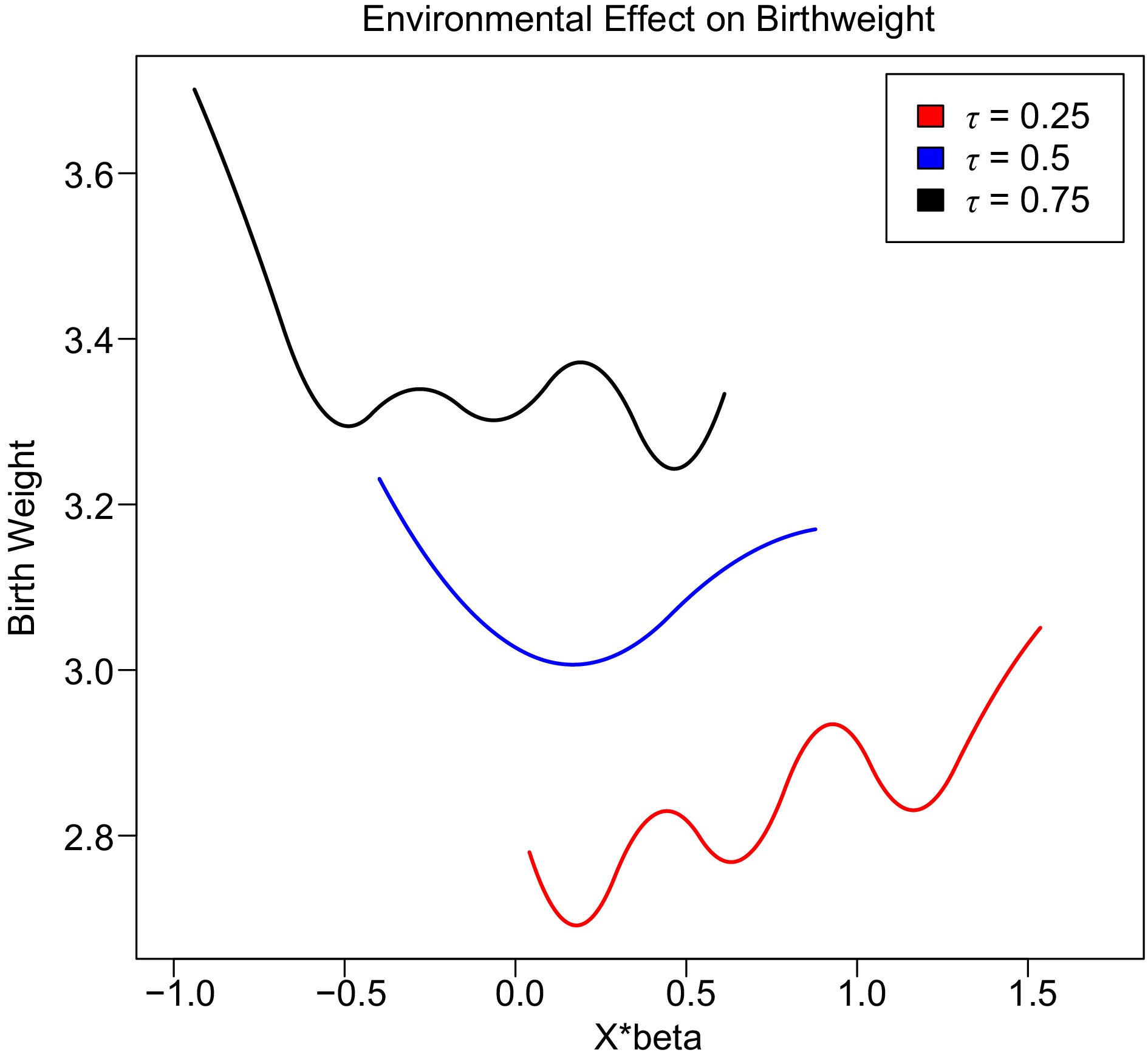
Figure 2.
Plot of environmental mixture index effect on birth weight.
Because the real-data analysis involved screening environmental variables, fitting the proposed model across 2,076 genes at three quantile levels, and repeating the analysis under different orderings of the environmental variables, multiplicity and selection stability are important considerations. In this study, the real-data analysis is intended as an illustrative application of the proposed method rather than a confirmatory genetic association analysis. Therefore, the identified genes and SNPs should be interpreted cautiously as exploratory findings. Future applications should incorporate formal multiple-testing adjustment, control of the false discovery rate, or resampling-based stability assessment to improve the reliability of biological conclusions.
-
VMICM provides a flexible framework for modeling nonlinear interactions between genetic variants
$ {\boldsymbol{G}} $ $ {\boldsymbol{X}} $ The proposed method accommodates high-dimensional genetic predictors through MCP penalization, enabling simultaneous classification of genetic variants into varying (interaction), constant (main effect), or zero effect categories. Simulation studies demonstrate strong finite-sample performance in both continuous and discrete genetic settings. The performance improves with increasing MAF, consistent with the greater statistical information available for common variants. The method also demonstrates stable performance under the simulation settings considered.
In the real-data application to birth weight, we identified genetic variants with quantile-specific main effects but found no evidence of nonlinear gene-by-mixture interaction with respect to the selected maternal environmental factors. This suggests that, within the studied population, genetic effects may act independently of the considered environmental mixture. However, the absence of detected interaction does not preclude interaction effects in other populations or under different environmental exposures. Moreover, nonlinear interaction effects generally require larger sample sizes to achieve adequate power, and future studies with larger cohorts may reveal additional structure.
The proposed framework involves multiple tuning parameters, including penalty parameters and spline approximation parameters. Although BIC-based selection demonstrated stable empirical performance in our simulation studies, the final model may still be sensitive to tuning parameter specification in certain settings. Developing formal sensitivity analysis procedures and investigating alternative tuning criteria, such as cross-validation or extended BIC, represent important directions for future research. In addition, although the proposed algorithm demonstrated stable empirical convergence across the simulation and real-data analyses, a formal theoretical investigation of identifiability, estimation consistency, oracle properties, and convergence guarantees is yet to be done for the proposed nonconvex penalized quantile optimization framework.
Several limitations of our study merit discussion. First, the identifiability constraints
$ \| {\boldsymbol{\beta}}\|_2 = 1 $ $ \beta_1 \gt 0 $ $ \beta $ Overall, the proposed quantile varying multi-index coefficient model provides a powerful and flexible tool for investigating heterogeneous genetic and environmental effects in complex trait studies, particularly when environmental exposures act as a mixture.
The authors thank the reviewers and editors for their constructive comments, which helped improve the quality and clarity of the manuscript.
-
The authors confirm their contribution to the paper as follows: study conception and design: Cui Y; methodological development: Guan S, Cui Y; data collection and preparation: Guan S, Cui Y; analysis and interpretation of results: Guan S, Zhang Y, Cui Y; draft manuscript preparation: Guan S; manuscript revision: Guan S, Cui Y. All authors reviewed the results and approved the final version of the manuscript.
-
The birth-weight data analyzed in this study were obtained from the Gene Environment Association Studies initiative (GENEVA), funded by the Genes, Environment and Health Initiative (GEI). Data access is subject to the policies and approval procedures of the original data repository. The data are not publicly distributed by the authors.
-
The authors declare that they have no conflict of interest.
-
accompanies this paper online at: https://doi.org/10.48130/stati-0026-0015.
- Supplementary File 1 Estimation algorithm and algorithm for the null model.
- Copyright: © 2026 by the author(s). Published by Maximum Academic Press, Fayetteville, GA. This article is an open access article distributed under Creative Commons Attribution License (CC BY 4.0), visit https://creativecommons.org/licenses/by/4.0/.
-
About this article
Cite this article
Guan S, Zhang Y, Cui Y. 2026. Quantile varying multi-index coefficient model for synergistic gene–environment interactions. Statistics Innovation 3: e014 doi: 10.48130/stati-0026-0015 

Quantile varying multi-index coefficient model for synergistic gene–environment interactions
- Received: 05 March 2026
- Revised: 06 June 2026
- Accepted: 01 July 2026
- Published online: 31 August 2026
Abstract: Gene–environment (G × E) interaction plays an important role in our understanding of complex traits, particularly when multiple environmental exposures act jointly as a mixture. Existing methods for studying continuous traits primarily focus on modeling conditional mean effects, whereas scientific and clinical interest often lies in identifying specific quantiles of the outcome distribution. We propose a penalized quantile regression framework for the varying multi-index coefficient model to investigate genetic effects and gene-by-mixture interactions across different quantiles. The method simultaneously identifies genetic variants with varying effects (interaction), constant effects (main effects), or no effect, while estimating environmental loading parameters within the mixture. By modeling multiple quantiles, the framework captures heterogeneous genetic and environmental effects along the response distribution. Simulation studies demonstrate accurate variable selection and robust estimation performance. In a real-data application to birth weight, the proposed approach identifies quantile-specific genetic main effects and heterogeneous environmental mixture effects, with limited evidence of nonlinear gene-by-mixture interaction. The proposed method provides a flexible and computationally efficient tool for high-dimensional G × E studies.