Early detection of tomato leaf spot and wilt diseases based on hyperspectral imaging technology

Tomato plants are highly adaptable and easy to cultivate, making them one of the most widely grown and economically significant vegetable crops worldwide^[1]. In recent years, driven by technological advancements and economic growth, tomato cultivation has garnered substantial support from governments, societies, and markets. Currently, China leads globally in both tomato cultivation area and yield, with tomato production and sales ranking among the top agricultural crops in the country. According to a survey by the International Organization of Seedkeepers, the global tomato cultivation area has surpassed 350 million hectares, with China accounting for an impressive 150 million hectares. Global tomato production exceeds 700 million tons, of which China contributes up to 400 million tons. Despite these achievements, tomato production faces significant challenges from various diseases, particularly leaf spot and wilt diseases, which severely impact yield. In modern agricultural practices, the targeted and rational application of pesticides is essential to ensure high-quality, high-yield production, and food safety. This approach not only effectively controls diseases but also minimizes environmental pollution caused by excessive pesticide use. However, the foundation for such targeted pesticide application lies in the accurate monitoring of plant growth and disease conditions, with early detection and precise identification of plant diseases being the most critical factors^[2]. Therefore, the early, rapid, and accurate diagnosis of vegetable diseases is vital for achieving high-quality, high-yield, and safe agricultural production. This is of great significance for promoting green, safe, and sustainable production of vegetables and fruits.

Hyperspectral imaging technology, an emerging method for crop disease detection, integrates imaging and spectral techniques to capture spectral data and analyze disease-related images. Researchers have achieved significant progress in disease detection using hyperspectral imaging, providing robust technical support for agricultural production. For instance, Wu et al. employed hyperspectral imaging to develop SPA2-ELM and CNN models for the early detection of soybean rust disease, as well as a CNN-SVM model for disease severity classification. After preprocessing and feature extraction, these models achieved test set accuracies of 87.5% and 92.08%, respectively^[3]. Similarly, Zhong utilized a bioluminescence system combined with hyperspectral imaging to monitor tomato bacterial wilt disease. By applying SNV preprocessing and SPA feature extraction, the high-throughput linear discriminant analysis model achieved a detection rate exceeding 90% for tomato bacterial wilt disease^[4]. In another study, Smigaj et al. investigated the optimal predictive factors for pine needle blight disease using hyperspectral data integrated with LiDAR technology. Their findings demonstrated that combining hyperspectral imaging and LiDAR significantly enhanced the detection capability for pine needle blight disease^[5]. Jaafar et al. further advanced the field by employing radial basis function neural networks to detect early and late stages of pumpkin powdery mildew disease, achieving detection rates of 82% and 99% under laboratory conditions^[6].

Despite these advancements, the majority of current research is confined to identifying and detecting a limited number of pathogens within a single crop or cultivation system, such as maize leaf spot disease and soybean powdery mildew disease. Few studies have explored dual diseases in a single crop, such as soybean anthracnose and bacterial blight^[7], or pests like aphids and red spider mites in cotton^[8]. These studies underscore the efficacy of hyperspectral imaging techniques integrated with machine learning and deep learning for crop disease detection. However, research on the early detection of plant diseases remains limited, particularly when phenotypic symptoms are not yet apparent. Early detection entails identifying diseases before visible symptoms appear on leaves—a task that traditional methods, such as manual visual inspection or single-band imaging techniques, often fail to accomplish due to their proneness to errors, time-intensive nature, and inability to deliver early, accurate, and rapid detection^[9].

In this study, we focus on leaf spot and wilt diseases, which are prevalent in tomato plants, as research subjects. By leveraging hyperspectral imaging technology combined with machine learning methods, we aim to detect these diseases at an early stage, enabling timely and effective disease control. The main research content and findings are summarized as follows:

(1) Multiple preprocessing and feature extraction methods were applied to process hyperspectral data, enabling the establishment of various early detection models. Through comparative analysis, the combination of processing methods with the highest detection performance was identified.

(2) The dung beetle optimization (DBO) algorithm was introduced to optimize the parameters of support vector machines (SVM), and bidirectional long short-term memory (BiLSTM) neural networks. This approach identified the optimal parameter configurations for each model, significantly enhancing the efficiency of tomato leaf spot and blight detection.

(3) A unified model capable of simultaneously detecting both diseases was developed, thereby improving disease identification efficiency. This achievement provides a robust foundation for targeted management of crop diseases.

This study employed the tomato variety 'Enira', with seedlings initially sourced from the Fengyuan Seed Company (Tai'an, Shandong, China). Due to the seedlings' robust disease resistance, pathogen inoculation experiments were conducted during the late seedling stage, prior to flowering and fruiting. The pathogens used in this study included Cladosporium fulvum, responsible for tomato leaf spot disease, and Fusarium oxysporum f. sp. lycopersici, responsible for tomato wilt disease. Suspensions of Cladosporium fulvum and Fusarium oxysporum f. sp. lycopersici were prepared for inoculation.

A total of 90 tomato plants exhibiting healthy growth and uniform size were selected for the experiment. These plants were divided into three groups: 20 plants served as the healthy control group, 35 plants were inoculated with Cladosporium fulvum via foliar spraying, and the remaining 35 plants were inoculated with Fusarium oxysporum f. sp. lycopersici via root irrigation. Following inoculation, the three groups were physically separated to prevent cross-contamination and maintained in a dark, humid environment for 12 h to facilitate successful pathogen establishment. Hyperspectral image acquisition was conducted 12 h post-inoculation.

The hyperspectral imaging system for tomato disease leaves was constructed using the SOC710VP® portable hyperspectral imaging spectrometer (SOC Inc., USA), as illustrated in Fig. 1. The system comprises a hyperspectral spectrometer, two symmetrically positioned halogen lamps, a diffuse reflectance standard whiteboard, an experimental platform, a dark box, and computer equipment.

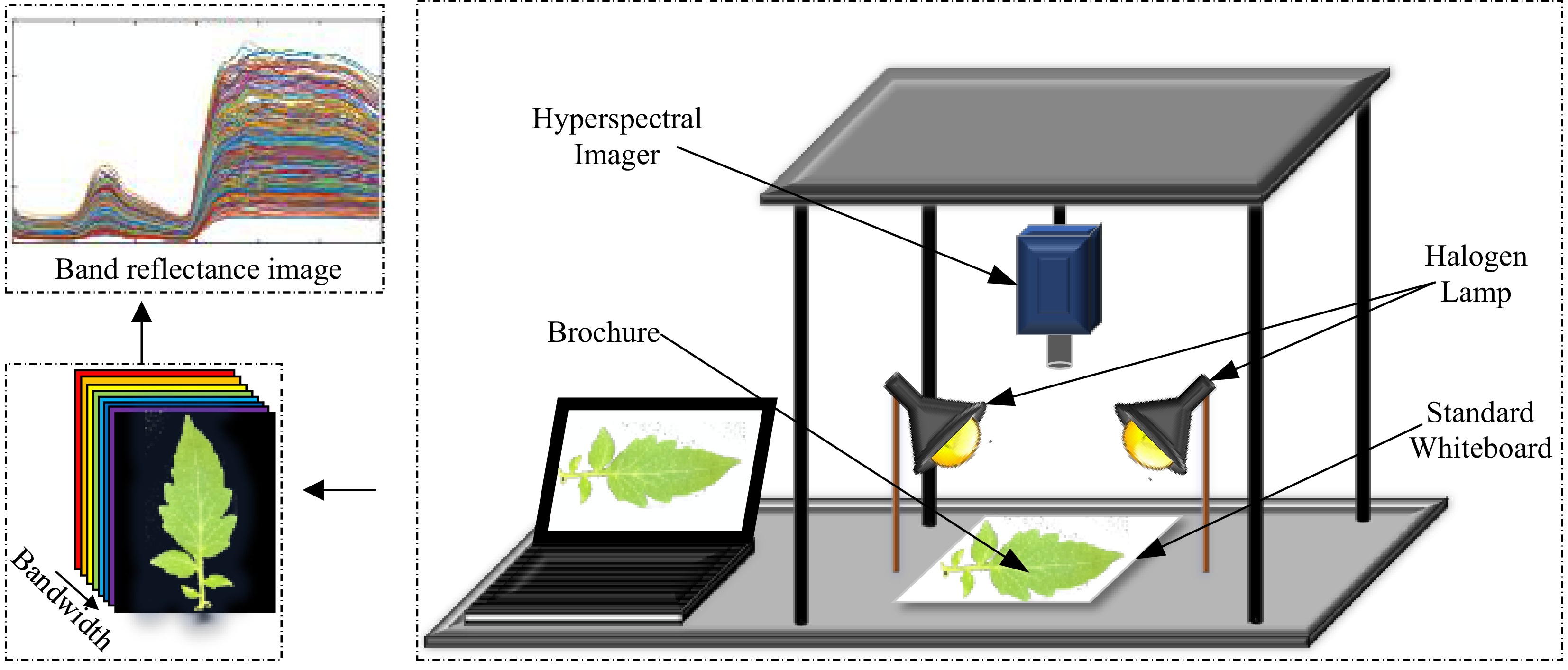
Figure 1. 

Hyperspectral data acquisition system.

To collect hyperspectral data from tomato disease leaf samples, a systematic procedure was followed. The hyperspectral camera was mounted on the experimental platform with the lens oriented vertically to ensure full coverage of the sample within the dark box. The halogen linear light source served as the sole illumination for the tomato leaves. Before data acquisition, the hyperspectral camera was preheated for 30 min to stabilize the current and intensity of the halogen light source. Hyperspectral images of the tomato disease leaves were then captured using the Hyper Scanner software, which is compatible with the hyperspectral camera.

To mitigate potential issues such as uneven light distribution from the halogen linear light source and dark current noise from the hyperspectral camera, black-and-white correction was applied to the acquired hyperspectral images^[10]. The reflection correction formula used is as follows:

where, F_w is the corrected whiteboard hyperspectral image, F_b denotes the hyperspectral image with all black and no light, F_s is the hyperspectral image to be corrected, and F is the corrected hyperspectral image.

After applying black-and-white correction, the hyperspectral images acquired using Hyper Scanner were processed with SRAnal for tasks such as image conversion and wavelength calibration. The processed images were then imported into ENVI for data extraction. Regions of interest (ROI) were defined by segmenting the hyperspectral images. In this study, the entire leaf area was selected as the ROI using ENVI's ROI tool, and the average reflectance within each ROI was calculated to represent the spectral data for a single sample. A total of 600 tomato leaf samples were collected, including 200 healthy leaves, 200 leaves infected with leaf spot disease, and 200 leaves affected by wilt disease.

The wavelength range selected for this study spans 400–1,000 nm. The visible light band (400–700 nm) primarily reflects chlorophyll content and the impact of disease on photosynthesis, while the near-infrared band (700–1,000 nm) is sensitive to changes in plant moisture status and structural integrity. This band is particularly responsive to water loss, tissue damage, and other physiological changes in leaves. Tomato leaf spot disease alters the moisture content and cellular structure of leaves, leading to distinct reflectance changes in the near-infrared band compared to healthy leaves. Similarly, wilt disease causes rapid water evaporation from tomato leaves, resulting in reduced water content and lower reflectance in the near-infrared band.

Hyperspectral data preprocessing methods

During the data acquisition process of the hyperspectral imaging system, external environmental factors and manual operations can introduce significant noise and interference into the collected hyperspectral data, adversely affecting the accuracy and reliability of subsequent modeling^[11,12]. To mitigate or eliminate the influence of interference and irrelevant information on hyperspectral data, thereby improving modeling accuracy, preprocessing of the hyperspectral data is essential^[13]. In this study, the primary preprocessing methods employed include Savitzky-Golay smoothing (SG), multivariate scatter correction (MSC), standard normal variate transformation (SNV), and derivative analysis (Der)^[14−16]. Given the challenge of directly determining the optimal preprocessing method for hyperspectral images, this study introduced a support vector machine (SVM) model to evaluate the effectiveness of different preprocessing techniques. SVM models were constructed using the preprocessed data, and their performance was compared to identify the most effective preprocessing method. The dataset is divided into training set, validation set, and test set in the ratio of 3:1:1, with 360 training samples, 120 validation set samples, and 120 test samples. Table 1 summarises the results of the comparative analysis.

Hyperspectral data feature extraction methods

The hyperspectral data of tomato leaf samples consist of 115 bands, some of which may negatively impact modeling efficiency. To enhance model performance and accuracy by eliminating redundant bands, this study employed four feature extraction techniques: Competitive Adaptive Reweighted Sampling (CARS), Successive Projections Algorithm (SPA), Uninformative Variable Elimination (UVE), and Principal Component Analysis (PCA). These methods were applied to reduce the dimensionality of the preprocessed hyperspectral data. By extracting meaningful spectral features and discarding irrelevant or redundant bands, these techniques aim to improve the speed and accuracy of model development and disease identification.

CARS is a feature variable selection algorithm developed by Li et al.^[17], which combines Monte Carlo sampling with Partial Least Squares Regression (PLSR) coefficients. In the wavelength variable selection process, CARS first calculates the weight of each wavelength variable using Adaptive Reweighted Sampling (ARS) technology, reflecting the contribution of each variable to the model. Subsequently, it identifies and removes wavelength variables with lower regression coefficient weights, iteratively refining the model to minimize the Root Mean Square Error of Cross-Validation (RMSECV). The CARS algorithm achieves optimal performance when the RMSECV value reaches its minimum^[18,19].

SPA is a forward variable selection algorithm designed to minimize covariance in vector space^[20−22]. It employs variable projection techniques for multivariate linear regression variable selection. The SPA process begins by randomly selecting an initial wavelength band for projection. It then iteratively projects one band onto the remaining bands, comparing the magnitudes of the projection vectors to identify the most informative wavelengths. Based on the size of the projection vectors, SPA determines the characteristic wavelengths. Finally, the calibration model is used to select the optimal set of feature wavelengths.

UVE is a classical spectral feature selection algorithm that introduces noise as irrelevant information to evaluate and identify informative variables in spectral data. Initially proposed by Centner et al.^[23,24], this method combines spectral variables with artificially generated noise to construct an augmented matrix of independent variables. By analyzing the statistical distribution of regression coefficients, UVE establishes upper and lower thresholds to filter variables that fall within these limits, thereby selecting the most relevant feature variables.

PCA, also known as the Karhunen-Loeve Transform or Hotelling Transform, is a method based on multivariate statistical techniques. It was first proposed by Pearson & Mag in 1901^[25], and subsequent researchers further developed the method using probability theory. There is a wide range of applications for PCA algorithms in areas such as model recognition and image processing^[26]. In different application areas, PCA is known by different names, including KL transform (Karhunen-Loeve Transform), Hotelling Transform, Subspace Approach, and Eigen-structure Approach^[27].

Early detection modeling methods

Bidirectional long- and short-term memory networks (BiLSTM)

The bidirectional long short-term memory network (BiLSTM) integrates the strengths of long short-term memory (LSTM) networks and bidirectional recurrent neural networks, enabling comprehensive bidirectional data modeling by capturing information flow from both forward and backward directions. The network comprises two independent LSTM layers: one processes data in the forward direction, while the other processes data in the backward direction. Each LSTM layer maintains its own hidden states and memory units, allowing it to capture contextual information from both temporal directions^[28].

During forward time steps, the first LSTM layer processes the input data, utilizing its hidden states and memory units to effectively capture forward contextual information. Simultaneously, during backward time steps, the second LSTM layer processes the input data in reverse, capturing backward contextual information using its independent hidden states and memory units. These two directional information flows are seamlessly integrated to form a more comprehensive representation, enabling the network to better understand the context and structure of the entire sequence^[29,30].

Through this bidirectional information flow mechanism, BiLSTM maximizes the utilization of data, resulting in more robust data parsing and significantly enhancing the performance and stability of the neural network. The structure of the BiLSTM neural network is illustrated in Fig. 2.

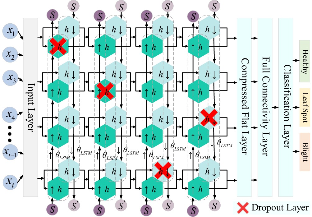
Figure 2. 

BiLSTM neural network structure.

As illustrated in Fig. 2, data flows into the BiLSTM layer through the input layer. The forward LSTM layer processes the input data sequentially from bottom to top, generating forward computational outputs $ \uparrow h $. Simultaneously, the backward LSTM layer processes the input data in reverse, from right to left, producing backward computational outputs $ h \downarrow $. To mitigate overfitting during training, a Dropout Layer is incorporated within the BiLSTM layer. After passing through the BiLSTM and Dropout layers, the data is further processed by a Flatten Layer, and a Fully Connected layer. Finally, a multi-class activation function is applied to classify and output the sample categories. The computational formula for the BiLSTM layer is as follows:

Where $ \uparrow h $ and $ h \downarrow $ represent the hidden states of the forward LSTM layer and the backward LSTM layer, respectively; y_t is the current output of BiLSTM; and f, w, and b correspond to the activation function, weight, and bias, respectively.

Dung Beetle Optimization Algorithm (DBO)

The Dung Beetle Optimizer Algorithm (DBO) was proposed by Xue & Shen^[31], drawing inspiration from the collective behaviors of dung beetle populations, including rolling, reproduction, foraging, and stealing. This algorithm leverages these behaviors to guide position updates and optimization strategies^[32]. Unlike traditional optimization methods, DBO classifies the population into four distinct types of dung beetles: rollers, breeders (responsible for forming dung balls), foragers (small dung beetles), and thieves. By integrating diverse position update mechanisms, DBO achieves comprehensive exploration of the search space and demonstrates strong capabilities in addressing complex optimization problems.

Roller dung beetle

Dung beetles exhibit two distinct rolling behavior patterns: unobstructed rolling and obstructed rolling. In the unobstructed rolling mode, the position update of the dung beetle is primarily influenced by the light source, as depicted in Fig. 3a. The position update during this mode is mathematically described by Eqn (3). However, when encountering obstacles during rolling, the dung beetle adjusts its orientation, and the corresponding position update is governed by Eqn (4).

where, t represents the current iteration number, X_i represents the position information of the i-th dung beetle at the i iteration, $\phi \in \left[ { - 1,1} \right]$ indicates the number of random natural factors, $k \in \left( {0,0.2} \right]$ represents the deflection coefficient constant, $b \in \left( {0,1} \right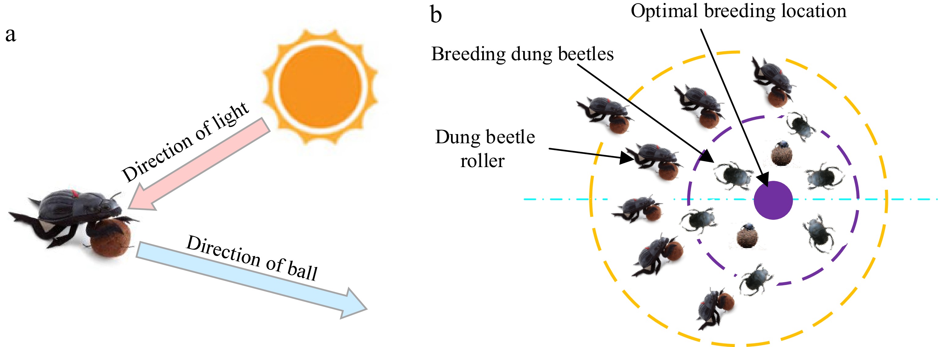)$ represents the coefficient constant, X^worse represents the worst position in the whole world, and $ \Delta X $ represents the luminous intensity.

Figure 3. 

Principles of Dung beetle movement. (a) Conceptual model of dung beetle trajectories. (b) Boundary selection strategy.

Breeding dung beetles

The breeding dung beetle selects a suitable area for oviposition based on the dung ball. Modeling the spawning area of female dung beetles, a range selection method is proposed, as illustrated in Fig. 3b. The method has the following mathematical model:

where, X^lbest indicates the optimal local position, Lb* and Ub* indicate the upper and lower limits of the spawning area, Lb and Ub indicates the minimum and maximum ranges of the optimization problem, R is the dynamic factor, and t_max is the maximum number of iterations.

Once the spawning area is identified, the dung beetles proceed to lay their eggs within this region. As indicated by Eqn (5), the parameter RR determines the boundary extent of the spawning area, with the boundary range dynamically adjusting as the value of R changes. Concurrently, the position of the breeding dung beetles is updated in response to the shifting boundary extent. This position update process is mathematically expressed as:

where, X_i(t) is the location of the i breeding dung beetle at the t iteration, b₁ and b₂ denote two independent random vectors of size 1 × N, N representing the dimensionality of the optimization problem.

Foraging dung beetle

Breeding and growing foraging dung beetles climb out of the ground in search of food, and the foraging dung beetles are guided by optimal foraging areas, which are also selected by applying the same boundary selection strategy model described above as shown in Fig. 3b. This mimics how dung beetles forage in nature. The extent of the optimal foraging area is defined as follows:

where, X^best denote the global best position, Lb^b and Ub^b denotes the minimum and maximum areas of the best foraging area, respectively, the locations of the foraging dung beetles have been updated as follows:

Where, x_i(t) represents the location information of the i small dung beetle at the t repetition, C₁ denotes a random number that follows a normal distribution, and C₂ represents a random vector belonging to (0,1).

Stealing dung beetle

The stealing dung beetle will search for the best food source and steal it, from Eqn (8) we can see that X^b is the best position, i.e., the best food source, so the position of the stealing dung beetle will be updated during the stealing process as the position of the best food source changes, the position is updated as follows:

where, x_i(t) represents the location information of the i-th thieving dung beetle at the t repetition, ω is a random vector of size 1 × D obeying a normal distribution, and η represents a constant.

Using the DBO algorithm and neural network models, this method iteratively improves the optimal solution and fitness by simulating the rolling, reproduction, foraging, and stealing behaviors observed in dung beetle populations. As the algorithm progresses through multiple iterations up to a specified maximum, it yields the global optimal solution alongside its corresponding best fitness, thereby determining the optimal parameters. Subsequently, these refined parameters are employed to train the neural network model using tomato leaf data, which in turn optimizes the detection and classification performance of the model.

Two evaluation metrics are employed: Accuracy, which measures the overall classification performance of the model, and Recall, which evaluates the model's ability to correctly identify specific disease types. Accuracy serves as the primary metric for assessing the model's classification effectiveness, while Recall acts as a supplementary metric. Recall is calculated using the following formula:

Accuracy: The proportion of correctly predicted samples relative to the total number of samples.

Recall: The proportion of correctly predicted samples in a specific category relative to the total number of samples belonging to that category.

where, x and y represent the number of correct predictions and the total number of samples, respectively; i represents the category; x_i represents the number of categories predicted to be i, which is the number of categories; and y_i represents the total number of samples in the i categories.

DBO parameter setting

For the DBO-optimized BiLSTM neural network, the three key optimization parameters are the number of hidden layer nodes, the initial learning rate, and the L2 regularization parameter. Once optimized, the optimal parameters are automatically integrated into the neural network for data training. The Dung Beetle Optimization algorithm is configured with a population size of 10 and a maximum iteration count of 20. Additionally, the BiLSTM model is trained for a maximum of 800 iterations using the Adam gradient descent algorithm, with the learning rate decay factor set to 0.1.

The collected hyperspectral images were processed to extract regions of interest, yielding a total of 600 tomato leaf samples, as shown in Fig. 4a, along with the average spectral profiles of tomato samples affected by different diseases, depicted in Fig. 4b. Analysis of the spectral curves reveals significant differences between healthy tomato leaves and those infected with wilt and leaf spot diseases. The overall and class-specific average reflectance curves exhibit distinct variations, providing a robust foundation for early detection research of tomato leaf spot and wilt diseases. Furthermore, to minimize the adverse effects of environmental disturbances on the study, preprocessing of the tomato leaf hyperspectral data is essential to improve detection accuracy.

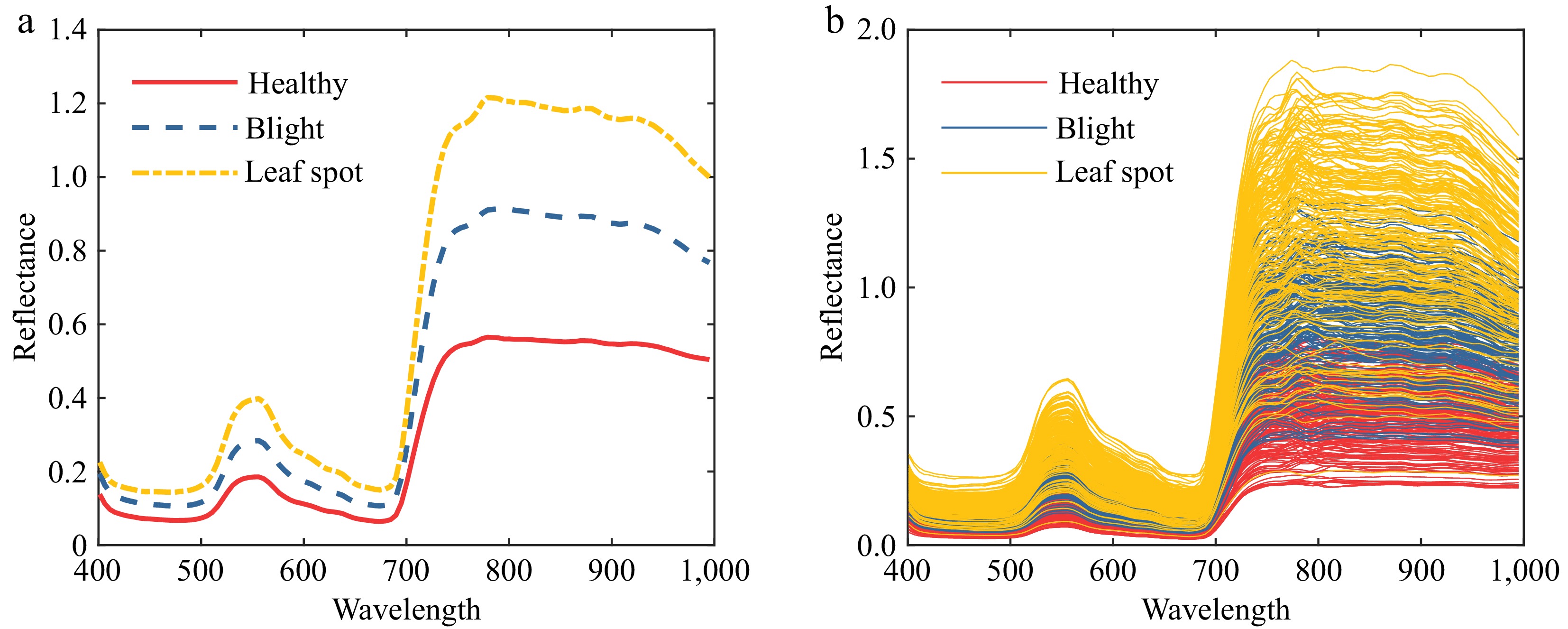
Figure 4. 

Tomato leaf reflectance curve. (a) Average reflectance curve of tomato leaves. (b) Raw reflectance curve of tomato leaves.

The SG algorithm is highly effective in denoising spectral data, reducing noise, and enhancing the signal-to-noise ratio. Meanwhile, the MSC and SNV methods excel in mitigating scattering effects caused by uneven sample distribution and varying particle sizes. Derivative processing further aids in eliminating baseline drift and smoothing background interference, thereby improving spectral recognizability. Given that the SG algorithm primarily focuses on smoothing and noise reduction, and other preprocessing methods such as differentiation may amplify noise in certain scenarios, the SG algorithm is adopted as the foundational method in this study. As illustrated in Fig. 5, combining the SG algorithm with MSC, SNV, and 1^st/2^nd derivatives effectively eliminates interference generated during spectral data acquisition.

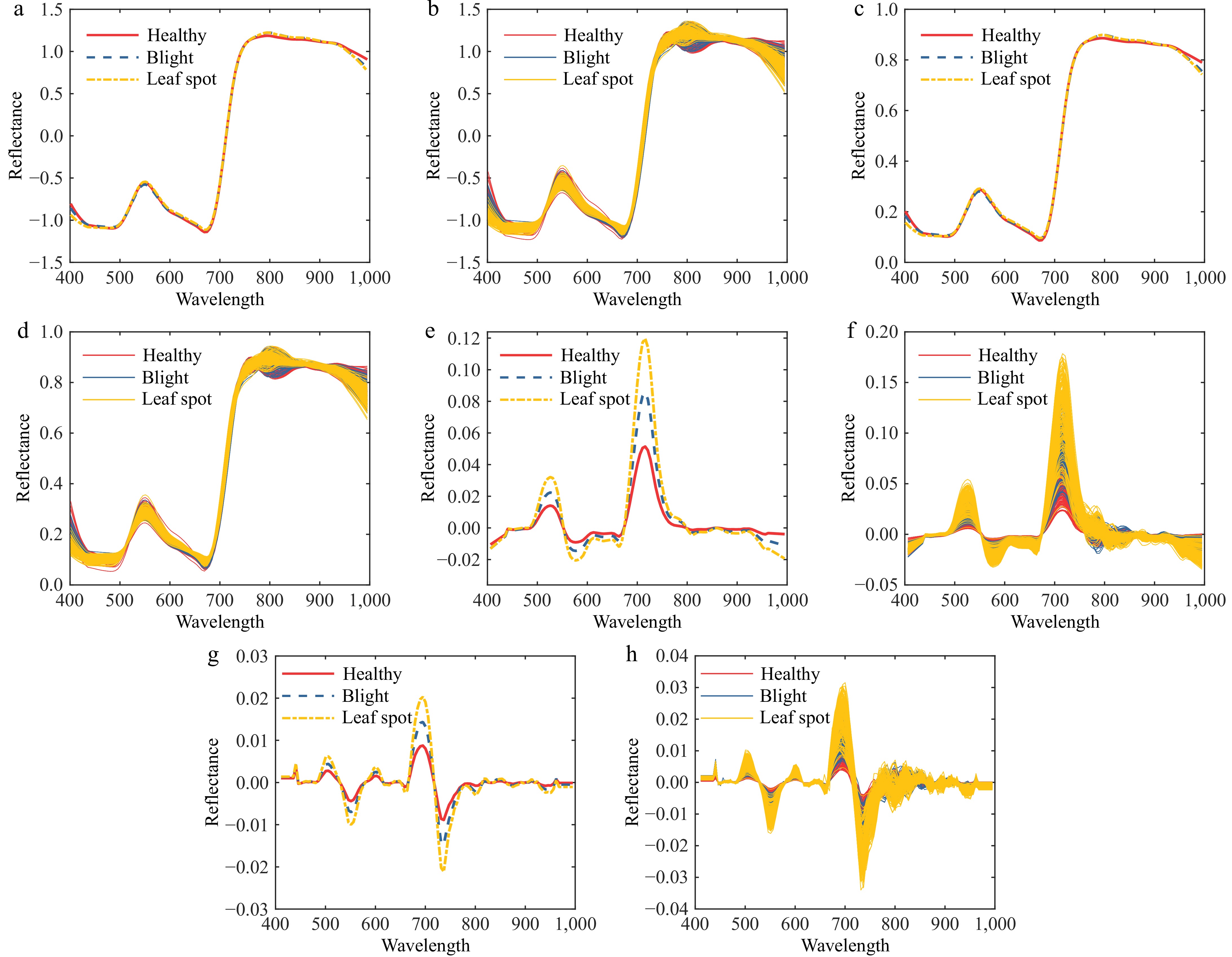
Figure 5. 

Spectral preprocessing map of diseased tomato leaves. (a) SNV-SG average spectral curve. (b) SNV-SG preprocessing. (c) MSC-SG average spectral curve. (d) MSC-SG preprocessing. (e) 1^st Der-SG average spectral curve. (f) 1^st Der -SG preprocessing. (g) 2^nd Der-SG average spectral curve. (h) 2^nd Der-SG preprocessing.

The classification performance of different preprocessing algorithms is presented in Table 1. Through a comparative analysis of the SG smoothing algorithm combined with various preprocessing methods, the 1^st Der-SG preprocessing algorithm achieves the highest overall detection accuracy of 79.3%. Consequently, the 1^st Der-SG preprocessing method is selected as the optimal preprocessing approach.

Hyperspectral feature wavelength extraction

CARS

Feature wavelengths were extracted from the hyperspectral data preprocessed using the 1^st Der-SG method, employing the CARS algorithm with a Monte Carlo sampling number of 50. The optimal feature wavelengths were determined by selecting the minimum value of the RMSECV.

As shown in Fig. 6a, the CARS feature wavelength extraction process achieves its minimum RMSECV value at the 27^th iteration. Beyond this point, the RMSECV does not exhibit significant changes but remains relatively stable until a sharp increase occurs around the 40^th iteration. This suggests that the wavelength set selected at the 27^th iteration represents the optimal feature wavelength set, comprising 13 feature wavelengths. The selected characteristic wavelengths are illustrated in Fig. 6b.

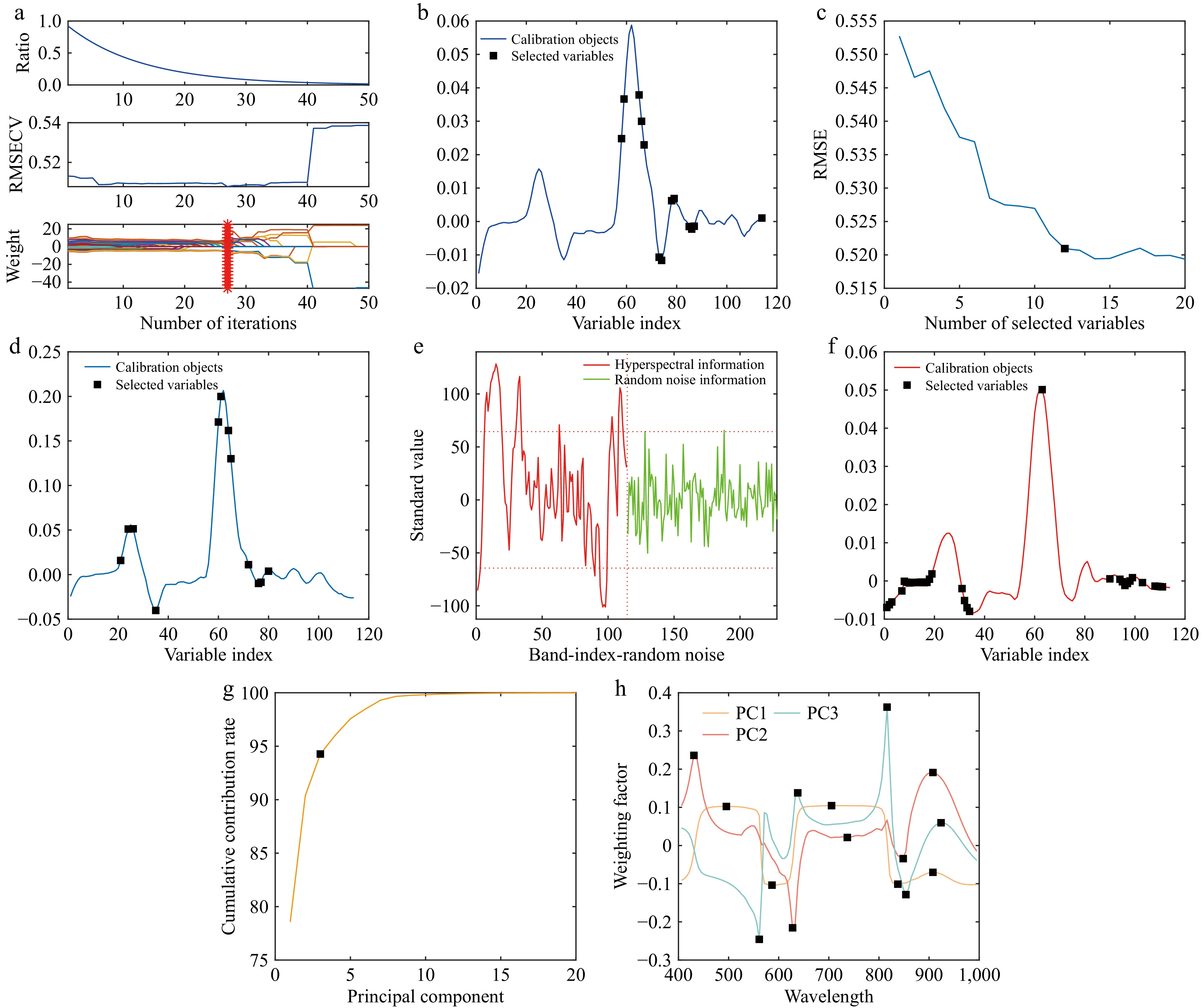
Figure 6. 

Characteristic wavelength selection. (a) CARS characteristic wavelength selection. (b) Distribution of feature wavelengths. (c) Represents the wavelength retention trend. (d) Distribution of feature wavelengths. (e) Spectral information screening. (f) Distribution of feature wavelengths. (g) Cumulative contribution curve. (h) Weighting factor curves.

SPA

When extracting feature wavelengths from the preprocessed data using the SPA algorithm, the dataset was first divided into a modeling set and a testing set in a 3:1 ratio, resulting in 450 samples in the training set and 150 samples in the test set. Following the division, the RMSE was calculated for different numbers of effective wavelengths, and the feature wavelengths were selected based on the minimum RMSE value. The results of the feature wavelengths extracted by the SPA algorithm are illustrated in Fig. 6d.

As shown in Fig. 6c, the SPA algorithm selects 12 bands when the RMSE decreases most rapidly, reaching a value close to the minimum. Beyond 12 bands, the RMSE decreases at a slower rate, indicating that 12 feature wavelengths are optimal. The distribution of these feature wavelengths is depicted in Fig. 6d, revealing that the wavelengths extracted by SPA are predominantly located at spectral peaks and valleys, exhibiting a dispersed pattern. Combined with Fig. 5, it is evident that the reflectance differences among the three types of tomato samples are most pronounced at these peaks and valleys.

UVE

The UVE algorithm begins by determining the optimal number of principal components based on the RMSECV values, where a smaller RMSECV indicates a more favorable number of principal components. However, due to the random generation of the noise matrix in each run and the inherent randomness of the algorithm, the selected number of principal components may vary. To address this variability and minimize random errors, the UVE feature selection process was performed over five iterations, starting with an initial set of 20 principal components. The results of these five iterations are visually summarized in Fig. 6f, which illustrates the minimum RMSECV values and provides detailed information on the selected number of principal components.

Analysis of Table 2 reveals that the optimal number of principal components varies across the five iterations, with values of 8, 12, 9, 11, and 7, respectively. The corresponding RMSECV values are 0.4789, 0.4794, 0.4775, 0.4793, and 0.4789, which are very close to each other. Considering the magnitude of the RMSECV values, the optimal number of principal components for UVE feature extraction is determined to be 9, as it corresponds to the smallest RMSECV value.

Once the optimal number of principal components is determined, feature selection is performed as illustrated in Fig. 6e. In the figure, the vertical dashed line separates the preprocessed tomato hyperspectral data from the random noise data. The left side represents hyperspectral information, while the right side corresponds to random noise. The horizontal dashed lines indicate the positive and negative thresholds for selecting hyperspectral information. Wavelengths exceeding the positive threshold or falling below the negative threshold are considered useful and selected for modeling, while those within the thresholds are classified as noise and excluded.

As shown in Fig. 6e, the UVE thresholds for noise addition are set at 67.5 and −67.5. The graph demonstrates that most data points lie within these thresholds, indicating that UVE primarily removes wavelengths from the central region of the data during feature extraction. This is further illustrated in Fig. 6f, where only one wavelength is selected between band numbers 40 and 90.

PCA

When employing the PCA algorithm for feature wavelength extraction, the initial step involves selecting the first few principal components that effectively capture the majority of the information from the three types of leaf samples, based on their cumulative contribution rate. Subsequently, by analyzing the weighting coefficients for each wavelength within these principal components, wavelengths corresponding to significant peaks or valleys in the weight coefficient curves are identified as the final feature wavelengths.

The process of determining the number of principal components in PCA is illustrated in Fig. 6g. The cumulative contribution rate of the first three principal components reaches 94.2694%, indicating that these components account for 94.2694% of the total dataset variance. Therefore, for PCA feature extraction, only the first three principal components are selected. Each principal component is assigned five feature points, resulting in a total of 15 feature wavelengths, as depicted in Fig. 6h.

Early detection modeling and analysis

After feature wavelength extraction, the complex information embedded in the tomato leaf hyperspectral images is condensed into a few dozen selected feature wavelengths. This reduction in the number of wavelengths significantly alleviates the computational burden on the model, thereby establishing a robust foundation for enhancing the classification accuracy, recognition capabilities, and stability of the early detection model^[33]. To identify the optimal model combination, the extracted feature data were divided into a training set and a validation set in a 3:1 ratio. Four models were constructed: SVM, DBO-SVM, BiLSTM, and DBO-BiLSTM. For the DBO-optimized SVM network, the two key parameters optimized are the penalty factor (C), and the radial basis function (gamma). For the BiLSTM neural network, the three optimized parameters are the number of hidden layer nodes, the initial learning rate, and the L2 regularization parameter. After optimization, the optimal parameters are automatically fed into the neural network for data training. The population size for the dung beetle optimization algorithm was set to 10, with a maximum of 20 iterations. Additionally, the BiLSTM model was trained for a maximum of 800 iterations.

The results of establishing early detection models for tomato diseases based on different feature extraction methods and models are summarized in Table 3. From the table, it is evident that models incorporating feature extraction demonstrate significant performance improvements compared to those relying solely on preprocessing, highlighting the critical role of feature extraction in enhancing the accuracy and reliability of tomato disease early detection. Among the different feature extraction methods, the SPA method exhibits lower accuracy on the test set across all four models compared to the other methods, suggesting that SPA's capability to extract relevant tomato disease features in this study is relatively limited. Notably, the UVE algorithm achieves the best detection results across all four models, with accuracies of 88.0%, 94.0%, 90.7%, and 97.3% for the SVM, DBO-SVM, BiLSTM, and DBO-BiLSTM models, respectively. This indicates that the UVE feature extraction algorithm is particularly well-suited for this study.

Analyzing the results for the three types of leaves, the detection accuracy for healthy leaves and those infected with early blight disease is relatively high across all four models, reaching approximately 90.0%. However, the performance for leaves infected with early wilt disease is notably lower, with only the DBO-BiLSTM model achieving an accuracy of 90.0%. This suggests that the internal physiological changes in tomato leaves during early wilt disease infection are less pronounced, making accurate classification more challenging.

Comparing the performance of different models, both models optimized by the DBO algorithm demonstrate significant improvements in detection accuracy. Specifically, the DBO-BiLSTM model outperforms the SVM, DBO-SVM, and BiLSTM models, achieving accuracies exceeding 90.0% across all feature extraction methods. The UVE feature extraction algorithm combined with the DBO-BiLSTM model achieves the highest detection accuracy of 97.3% on the test set, while the CARS, SPA, and PCA methods combined with the DBO-BiLSTM model achieve accuracies of 96.0%, 94.7%, and 96.0%, respectively. This underscores the superior performance of the DBO-BiLSTM model. Based on the comprehensive analysis, the 1^st Der-SG-UVE-DBO-BiLSTM model combination demonstrates the best detection performance, achieving an overall accuracy of 97.3% on the test set. The recall rates for detecting healthy tomatoes, wilted tomatoes, and tomatoes with leaf spots are 100.0%, 94.0%, and 98.0%, respectively. The detection results are visualized in Fig. 7.

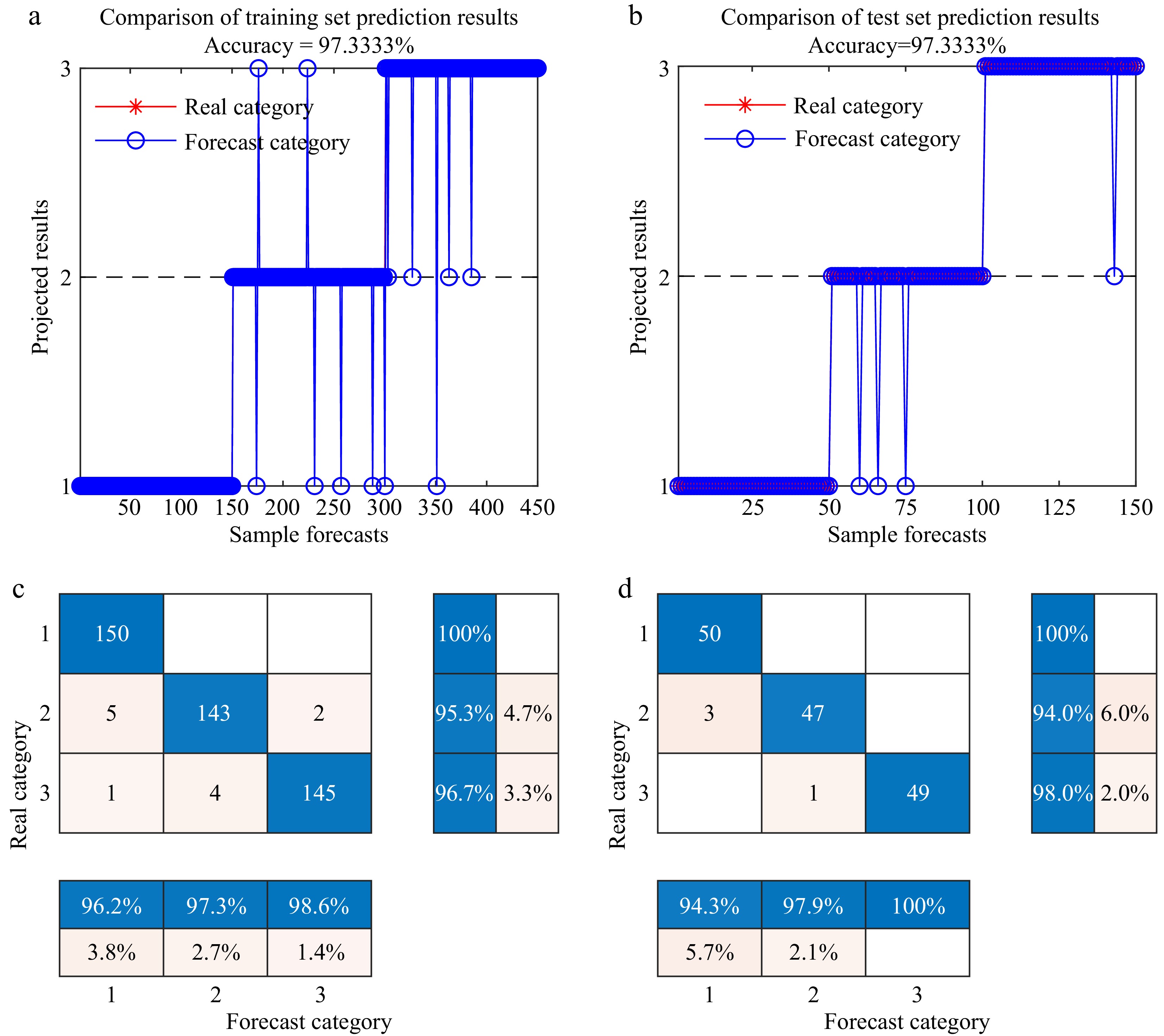
Figure 7. 

1^st Der-SG-UVE--DBO-BiLSTM Detection Classification Result. 1, 2, and 3 represent healthy, infected early wilt, and infected early leaf spot leaves of tomato, respectively. (a) Training set line chart. (b) Test set line chart. (c) Confusion matrix plot for the training set. (d) Confusion matrix plot for the test set.

In this study, after processing the hyperspectral data using four preprocessing methods—1^st Der, MSC, SNV, and SG—the model with 1^st Der-SG preprocessing achieved the highest accuracy on the test set. This advantage can be attributed to the inevitable presence of instrumental noise during hyperspectral data acquisition, as well as the physical changes in samples over extended periods under varying environmental conditions, which lead to spectral baseline drift. Baseline drift significantly impacts model recognition performance. In contrast, the scattering effect caused by uneven particle size and distribution in tomato samples is relatively minor, making scattering correction methods less effective than baseline correction.

The superior performance of 1^st Der over 2^nd Der is due to the primary function of the first-order derivative, which is to eliminate low-frequency noise (e.g., baseline drift) and emphasize spectral trends. By calculating the slope of the spectral curve, the first-order derivative highlights changes in absorption peaks or inflection points, which are often closely associated with substance composition or disease characteristics. On the other hand, while the second-order derivative also removes low-frequency noise, it further amplifies high-frequency changes in the spectral data, such as sharpening absorption peaks. However, the second-order derivative can inadvertently amplify high-frequency noise (e.g., random fluctuations or measurement errors), leading to suboptimal results, especially when processing noisier data.

UVE feature extraction for further analysis

In the feature extraction process, the UVE algorithm demonstrates optimal modeling performance, achieving a recall rate of 100% for healthy samples. This superior performance is attributed to the UVE algorithm's higher robustness compared to CARS, particularly when handling noisy data such as spectral data. By eliminating uninformative variables, UVE effectively reduces the impact of noise on feature selection. Additionally, UVE does not rely on large-scale sampling competition during variable selection, making it more suitable for small-sample modeling scenarios like this study.

In contrast to the SPA algorithm, which selects variables stepwise to maximize orthogonality among them, UVE performs better for data with nonlinear relationships, such as hyperspectral data. Furthermore, compared to PCA, which primarily focuses on dimensionality reduction and may inadvertently lose important spectral features, UVE emphasizes variable selection, ensuring the retention of critical spectral information.

Some limitations of this study

The experimental environment in this study was relatively controlled, with all samples collected indoors after uniform cultivation and inoculation. While this approach ensured consistency, it may have influenced the experimental results. Future research could expand the scope by collecting hyperspectral images of tomato leaves grown under field conditions. This would allow for the analysis of spectral data in more complex environments and facilitate real-time detection of tomato leaf spot and wilt diseases.

Due to experimental limitations, this study focused solely on tomato leaf spot and wilt diseases. Future work could extend the research to include other prevalent diseases, such as early blight, late blight, and gray mold, or explore alternative crops like eggplant and peppers. Implementing intercropping models for multiple crops and diseases could enable simultaneous detection and classification, supporting timely disease management and enhancing crop yield and quality.

This study focused on tomato plants, specifically targeting common diseases such as leaf spot and wilt. Hyperspectral imaging technology was employed to capture hyperspectral images of tomato leaves in the early stages of disease development. After extracting and processing the hyperspectral data, an early detection model was developed capable of non-destructively detecting and classifying tomato leaf spot and wilt diseases simultaneously. The key findings of this research are summarized as follows:

(1) Raw spectral data were preprocessed using four methods: 1^st/2^nd derivative (Der), multivariate scatter correction (MSC), standard normal variate transformation (SNV), and Savitzky-Golay smoothing (SG). Modeling analysis demonstrated that the 1^st Der-SG preprocessing method outperformed the others for detecting early-stage tomato diseases, achieving an accuracy of 79.3%. Feature extraction was performed on the preprocessed data using CARS, SPA, UVE, and PCA, yielding 13, 12, 33, and 15 feature wavelengths, respectively, for the 1^st Der-SG data.

(2) The DBO optimization algorithm was applied to optimize the penalty factor (c) and radial basis function parameter (g) for SVM, as well as the number of hidden layer nodes, initial learning rate, and L2 regularization parameter for BiLSTM. The resulting DBO-SVM and DBO-BiLSTM models exhibited significantly improved performance compared to the standalone SVM and BiLSTM models.

(3) Among the various model combinations, the 1^st Der-SG-UVE-DBO-BiLSTM model demonstrated the best detection performance. It achieved an overall accuracy of 97.3% on the test set, with recall rates of 100.0%, 94.0%, and 98.0% for healthy, wilted, and spotted tomato plants, respectively. This model provides robust technical support for the early detection of tomato leaf spot and wilt diseases and establishes a theoretical foundation for the simultaneous detection of multiple diseases.