Quantifying the difference between supply and demand of ecosystem services at different spatial-temporal scales: A case study of the Taihu Lake Basin

ESs refers to all kinds of benefits humans get directly or indirectly from the ecosystem^[1]. ESs are split into support, regulation, supply, and cultural services^[2]. At the same time, it is found that 15 of the 24 types of ESs have been degraded and unsustainable. This accounts for about 60% of the total number of assessments^[3]. It is predicted that the degradation of ESs will deteriorate significantly in the first half of the 21^st century. Through the research of ESs, we can improve our understanding of the ecological functions, interactions, and interdependencies within and between ecosystems^[4]. Stakeholders, especially policy-makers and implementers at the national and provincial levels, have high expectations for targeted scientific research on ESs, hoping to provide reliable information and technology to assess and predict the ecological consequences of their decisions and support and optimize them^{[2, 5]}. Empirical research on ESs is essential to determine the benefits of ecological restoration and support its use in natural resource management to achieve a balance between economic and urban growth without causing irreversible degradation risk of ESs^{[6, 7]}.

Human activities have led to a mismatch between supply and demand for ESs. ESs supply can be described as the capacity of natural ecosystems to provide services or goods for human well-being^{[8, 9]}, ESs demand can be defined as the willingness to pay for access to or protection of certain ESs^{[10, 11]}. Some scholars also believe that demand is an ESs that is consumed or used within a specific time and space range^[12], or the ESs that we desire^{[8, 13]}. Understanding the relationship between the supply and demand of ESs is critical to studying ESs and an essential basis for pushing ESs from theory to management practice and policy design^{[7, 14, 15]}. However, increased ESs demands with rapid human activities^[16−18], e.g., urbanization, deforestation, and population expansion, have resulted in the shortage of ESs supply and a high mismatch between the supply and demand of ESs from regional to national scales^[13]. Therefore, the supply and demand of ESs have become the focus of international research on ESs^{[13, 19]}. Assessing and revealing the difference between the supply and demand of ESs can provide relevant insights for improving human well-being^[20−24], and support decision-making for reflecting the spatial allocation of environmental resources in rapidly urbanizing regions or countries.

The ESs supply and demand mechanisms across different spatial-temporal scale changes are still unclear. Territorial administrative divisions follow a clear hierarchical structure. The differences in administrative levels determine the power of management and decision-making, the ability to attract the central government and foreign investment, and the role of local governments^{[25, 26]}. These three factors interact with each other and affect the participation of cities in regional coordinated development^[26−28]. Due to the different spatial resolutions of satellite data and increased demands for decision-making at different spatial scales^[29−31], there are many studies conducted on the supply and demand of ESs at different spatial scales^[32−34]. But the supply and demand of ESs will be changed by an imbalance of economic development and spatial heterogeneity of geographical or ecological systems over temporal and spatial scale changes^{[23, 24, 35, 36]}. Quantifying the correlation characteristics of ESs and coordinating the relationship between the supply and demand of ESs at different temporal-spatial scales is the key to revealing the relationship between different ESs at various spatial-temporal scales^[37−39] and is also an important basis for management decision-making. However, previous studies mainly focused on the spatial scale difference of the supply and demand of ESs at a single period and neglected the effect of spatial-temporal changes on the supply and demand of ESs^{[16, 37, 38]}

TLB is the core part of the Yangtze River Delta in China. Rapid industrialization and urbanization have significantly changed the land use of the basin and caused environmental degradation, posing a great threat to ecological security and a significant challenge to the region's sustainable development. Therefore, it is urgent to evaluate the ecological environment of TLB to promote scientific development in this region. Previous studies have assessed the ecological risks in the basin from 1985 to 2020^[40]. Land use influences supply and the factors that influence them are examined^{[41, 42]}. Evaluation of TLB ESs from pixel and county scales, and the trade-off between these indicators^[37]. Simultaneously, the difference between ecosystem supply and demand in the Yangtze River’s middle and lower reaches was assessed on a larger scale^{[24, 43]}. Although their research assessed the difference between supply and demand in TLB, it lacked an assessment of the scale of Chinese towns, counties, and cities. Therefore, it is the key to realizing the sustainable development of society and nature in TLB to study the changes in supply and demand of ESs from the perspective of time and space changes and multi-stakeholders as well as to formulate a sustainable supply model to meet the needs of ESs.

Taking TLB as an example, this study investigated the supply and demand of five ESs between 2010 and 2020, including water yield, carbon sequestration, recreation, food production, and heat regulation, in order to improve the understanding of the supply and demand of ESs in TLB and to explore its supply and demand situation from different administrative scales, with the aim of providing more reliable countermeasures and suggestions for various stakeholders and managers to make decisions on ecosystem management. Specific objectives of the work were to: (1) The quantitative and spatial characteristics of supply and demand of five ESs indicators in TLB in 2010 and 2020 were analyzed using the InVEST model and map overlay. (2) Analyze the supply and demand pattern of ESs at different scales from pixel scale, township scale, county scale, and city scale. (3) Provide advice to policymakers and decision-makers at different management scales.

TLB is located at 119°3′1″–121°54′26″ E, 30°7′19″–32°14′56″ N, and has an area of approximately 3.69 × 10⁴ km², as shown in Fig. 1. It has a north subtropical monsoon climate with an average annual temperature of 15–17 °C, with the highest temperature of 37–39 °C in August. The average annual precipitation is 1,552 mm^{[44, 45]}. In 2020, TLB's total population was 67.55 million, accounting for 4.8% of China's total population, a regional GDP of 9,997.8 billion-yuan, accounting for 9.8% of China's GDP, and a per capita GDP of 148,000 yuan^[46]. Since ancient times, TLB has been an important grain producing area as well as an important area for economic development in China. With a large population and rapid urbanization, it has big cities such as Shanghai, Suzhou, and Hangzhou.

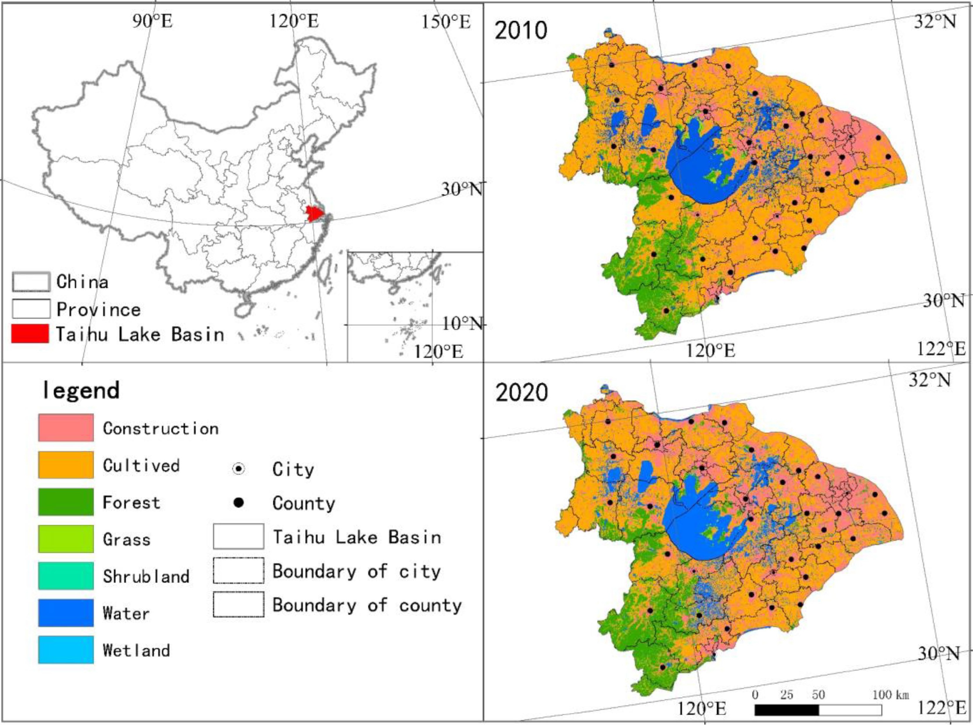
Figure 1. 

Location of TLB in the Yangtze River Delta in China.

Data source

This study used seven geospatial and statistical data sets, including administrative boundaries, the Digital Elevation Model (DEM), climates, soil property, land use, population, and statistical data. The resolution and source of each data used in this study are shown in Table 1 for climate (precipitation, temperature, and evapotranspiration) and some statistical data (water requirement, carbon emissions, per capita green area, food production and consumption). Due to the different resolutions of the original data variables, it is necessary to transform the data into a consistent scale research unit of 30 m × 30 m.

Ecosystem services

Methodological framework

We have comprehensively considered the vital ecological processes and other relevant literature in the TLB^{[14, 41, 47]}. And conduct field research on TLB. We choose the indicators of ESs supply and demand according to the following criteria: (1) The widely recognized ESs framework^{[3, 22]}; (2) It is closely related to residents' social and economic activities, residents, and their health^{[30, 31, 48]}; (3) Reflect the preferences and interests of policymakers and managers^[1]. (4) Data availability. Specific methods are described in Supplemental File 1.

This study selected the following ESs indicators: (1) Water yield service; (2) Carbon sequestration service; (3) Recreation service; (4) Food production service; and (5) Heat regulation service. Specifically, water, food, recreation and high temperature are important indicators of human life and health in the TLB. Green recreational spaces can effectively regulate the pressure of human life. Water and carbon are fundamental resources for industrial productivity. The global challenge of climate change is essentially related to carbon sequestration and heat regulation services. These indicators of ESs are also directly associated with the supply and demand for further ESs. The supply and demand for each ESs are first quantified at the pixel scale and subsequently at township, county, and city scales in 2010 and 2020. Different scales represent different administrative levels of ESs in TLB, the pixel scale represents exemplary management in TLB, and towns, counties, and cities are administrative levels with varying responsibilities in China.

The analysis framework for exploring the spatial pattern and scale effect of supply and demand among five ESs in TLB. (1) Data preparation, such as specific methods are referred to in Table 1, which lists the data sources and resolutions used in this study. All the data used are resampled into pixels with a spatial resolution of 30 m × 30 m. (2) Evaluation of ESs: Statistical model analysis and spatialization are made with the help of Arcgis10.6 software(version: 10.6.0.8321). The InVEST model is used to evaluate the supply of water yield and carbon sequestration^[49]. The parameters used in the model simulation are all based on the operation manual and similar literature in relevant regions^[14]. Specific methods are referred to in Supplemental File 2. (3) Based on the evaluation results, it shows the spatial and temporal changes of five ESs indicators in TLB and analyzes the mismatch between the supply and demand of ESs at different scales. (4) According to the scale effect of ESs supply and demand, ecosystem management suggestions of decision-makers at different levels are put forward.

ESs supply and demand quantification

(1) Water yield service

Water yield supply was calculated using InVEST. Water yield demand is collected from the bulletin of water resources in TLB, which provides information on water use, including agricultural water, industrial water, domestic water, and ecological water. It assigns water consumption to cultivated land, construction land, and ecological land (forest land and grassland). Specific details are referred to in Supplemental File 1.1. Water supply and demand for services are calculated using the following formula:

Where Equation 1 is supply and demand for water yield services, respectively; $ P $ is annual precipitation; $ ET $ is annual evapotranspiration; where Equation 2 is demand for water yield services, $ {D}_{\mathrm{a}\mathrm{g}\mathrm{r}\mathrm{i}\mathrm{c}\mathrm{u}\mathrm{l}\mathrm{t}\mathrm{u}\mathrm{r}\mathrm{a}\mathrm{l}} $, $ {D}_{industrial} $, $ {D}_{\mathrm{d}\mathrm{o}\mathrm{m}\mathrm{e}\mathrm{s}\mathrm{t}\mathrm{i}\mathrm{c}} $, $ {D}_{\mathrm{e}\mathrm{c}\mathrm{o}\mathrm{l}\mathrm{o}\mathrm{g}\mathrm{i}\mathrm{c}\mathrm{a}\mathrm{l}} $ are actual water use in agriculture, industry, household, and ecological, (m³), respectively.

(2) Carbon sequestration service

The InVEST model estimates carbon sequestration using land use and carbon storage of above ground biomass, underground biomass, soil, and dead organic matter. The demand for carbon sequestration mainly comes from the energy consumption of households, services, and industries in the statistical yearbook, with the unit of ten thousand tons of standard coal. This carbon consumption is assigned to the corresponding land use. Specific details are referred to in Supplemental File 1.2. The following equation is used to calculate the supply and demand for carbon sequestration:

Where, Equation 3 is carbon sequestration service supply (ton), expressed as total carbon sequestration, $ {C}_{\mathrm{a}\mathrm{b}\mathrm{o}\mathrm{v}\mathrm{e}} $ is aboveground carbon sequestration (ton), $ {C}_{\rm{under}} $ is underground carbon sequestration (ton), $ {C}_{\rm{soil}} $ is soil carbon sequestration (ton), $ {C}_{\rm{dead}} $ is cadaver organic matter carbon sequestration (ton). Equation 4 is carbon sequestration service demand, $ {E}_{\mathrm{s}\mathrm{e}\mathrm{r}\mathrm{v}\mathrm{i}\mathrm{c}\mathrm{e}\mathrm{s}} $， $ {E}_{\rm{industrial}} $，and $ {E}_{\mathrm{d}\mathrm{o}\mathrm{m}\mathrm{e}\mathrm{s}\mathrm{t}\mathrm{i}\mathrm{c}} $ are actual carbon emissions from industrial enterprises, services, and households, respectively.

(3) Recreation service

Recreation is provided by evaluating residents' available green space areas in TLB. Recreation demand is defined as the per capita green space area of residents counted by the government in the statistical yearbook. Specific details are referred to in Supplemental File 1.3. Supply and demand are calculated using the following equation:

Where Equation 5 is recreation supply (hm²/hm²). ${A}_{Greenspace, Grid}$ is the area of green space (Woodlands, grasslands, water bodies, and wetlands) in a grid (hm²). ${A}_{Grid}$ is an area per grid area (hm²). Equation 6 is recreation demand (hm²/hm²). $ {A}_{Guided\;Greenspace} $ is the government guidance on green space provision, which is 0.00135 hm²/person according to the Ecological Garden City Standard.

(4) Food production service

The food supply and demand in this study are estimated by the statistical yearbook. We add the output of food crops, oil crops, fruits and vegetables, meat, eggs, milk, and freshwater products in each city. Then we used to interpolate them into the land use grid data for cultivated land, grassland, water body, and wetland, respectively. For food demand, we can estimate it by multiplying the population density by per capita food consumption. Specific details are referred to in Supplemental File 1.4. Supply and demand are calculated using the following equation:

Where Equation 7 is food production demand (ton/hm²); $ {p}_{i,j} $ is the annual production of j type products, such as grain, oil plants, meat, and aquatic products. Find food production in the statistical yearbooks of different cities (ton). Assign grain, oil crop, vegetable, and fruit yields to arable land (ton/hm²); Assign meat, egg, and milk yields to grasslands (ton/hm²); Assign freshwater products to wetlands and water bodies (ton/hm²). Where Equation 8 is food production demand (ton/hm²); $ {P}_{POP} $ is population density (population/hm²); $ {P}_{eru} $ and $ {P}_{err} $ are the per capita food consumption of urban areas and rural areas, respectively (ton/person). The values of $ {P}_{eru} $ and $ {P}_{err} $ were calculated according to the statistical yearbook of the four provinces and their subordinate cities in the TLB.

(5) Heat regulation service

The temperature difference between each grid and the regional average calculates the service supply. According to the spatial distribution of local vulnerability, the demand for heat regulation is determined. The characteristics of urban vulnerability are the number of exposed people and the number of particularly sensitive people in each urban block. Specific details are referred to in Supplemental File 1.5. Heat regulation supply and demand are calculated using the following equation:

Where Equation 9 is heat regulation supply, (°C), $ {T}_{\mathrm{m}\mathrm{e}\mathrm{a}\mathrm{n}} $ it is the mean max air temperatures of the study area in August, (°C); $ {T}_{\mathrm{G}\mathrm{r}\mathrm{i}\mathrm{d}} $ is the max air temperatures per grid, (°C); Equation 10 is heat regulation demand, (°C); ${{P}_{Grid}}$ is the population of the grid; ${A}_{\mathrm{G}\mathrm{r}\mathrm{i}\mathrm{d}}$ is the area of the grid; ${{P}_{Age}}$ is the population of children under 4 years and older people over 65 years in the grid, $ {T}_{\mathrm{M}\mathrm{i}\mathrm{n}} $ is the lowest value of the max air temperatures of all grids in the study area, (°C).

（6）Ecological supply-demand ratio

Ecological Supply-Demand Ratio (ESDR) compares ESs's actual supply and demand with human needs and can be used to reveal the surplus or deficit of ESs^[44]. In addition, the comprehensive supply-demand ratio (CESDR) is calculated as the arithmetic average of ESDR, which is used to evaluate ESs at the comprehensive level^[9]. Through these two indicators, the relationship between the supply and demand for ESs is analyzed.

Where in Equation 11, S and D refer to the actual supply and demand for specific ESs, respectively, and $ {S}\mathrm{m}\mathrm{a}\mathrm{x} $ and ${D}\mathrm{m}\mathrm{a}\mathrm{x} $ are the maximum values of ESs supply and demand, respectively. A positive $ ES DR $ indicates an ESs surplus, a negative $ ES DR $ is an ESs shortfall, and a zero $ ES DR $ is a balance between ESs supply and demand.

Where in Equation 12, n is the number of estimated ESs, with n = 5 in this case, and $ ES DRi $ is the supply-demand ratio for each ESs type. Based on the actual situation, we believe that all five ecosystem indicators are equally relevant. So, when calculating the $ CES DR $ value, they are all weighted at 1.

Scales analysis

The magnitude of benefits humans derive from ecosystems is closely related to the spatiotemporal scale of the ecosystem. There is currently a lack of research on supply and demand. The scale feature of ESs is the combination of society and ecology. Human development datasets are often at the scale of jurisdictions, such as a counties, cities, provinces, or countries^[28]. There is no essential causal scale relationship between the ecosystem and human level, although both can be mapped independently into a common space-time domain. Therefore, it is necessary to consider the supply and demand of ESs from the administrative hierarchy scale.

The TLB has 792 towns, 74 counties, and 13 cities. Select pixel, township, county, and city scales to evaluate ESs. Among them, 30 × 30 m pixels are selected as the data source. After the pixel scale calculates supply and demand, 2,000 randomly generated points are used to gather the pixel scale data and analyze the pixel scale characteristics. We extract, analyze, and compare the characteristics of supply and demand based on administrative vector boundaries of towns, counties, and cities in TLB.

Extract data from different grades for the T-test and correlation analysis. When the p value is less than 0.05, it is considered to have a significant influence. When the p value is less than 0.01, it is highly significant. When the p value is less than 0.001, the significance is the highest.

(1) Water yield service

In 2010, the total water supply in TLB was 96.66 billion m³, while the total water demand was 118.59 billion m³, and the gap between supply and demand was 21.93 billion m³. In 2020, the total water supply in TLB was 94.46 billion m³, while the total water demand was 141.12 billion m³, and the gap between supply and demand was 46.66 billion m³.

There is also a spatial mismatch between supply and demand. As shown in Fig. 2, from 2010 to 2020, the abundant supply is mainly concentrated in the woodland areas in the northwest and southwest of TLB. High demand areas primarily focus on the densely populated north, east, and southeast areas. The regional water supply service in the south is gradually decreasing, while areas with high water demand in the east and middle are increasing.

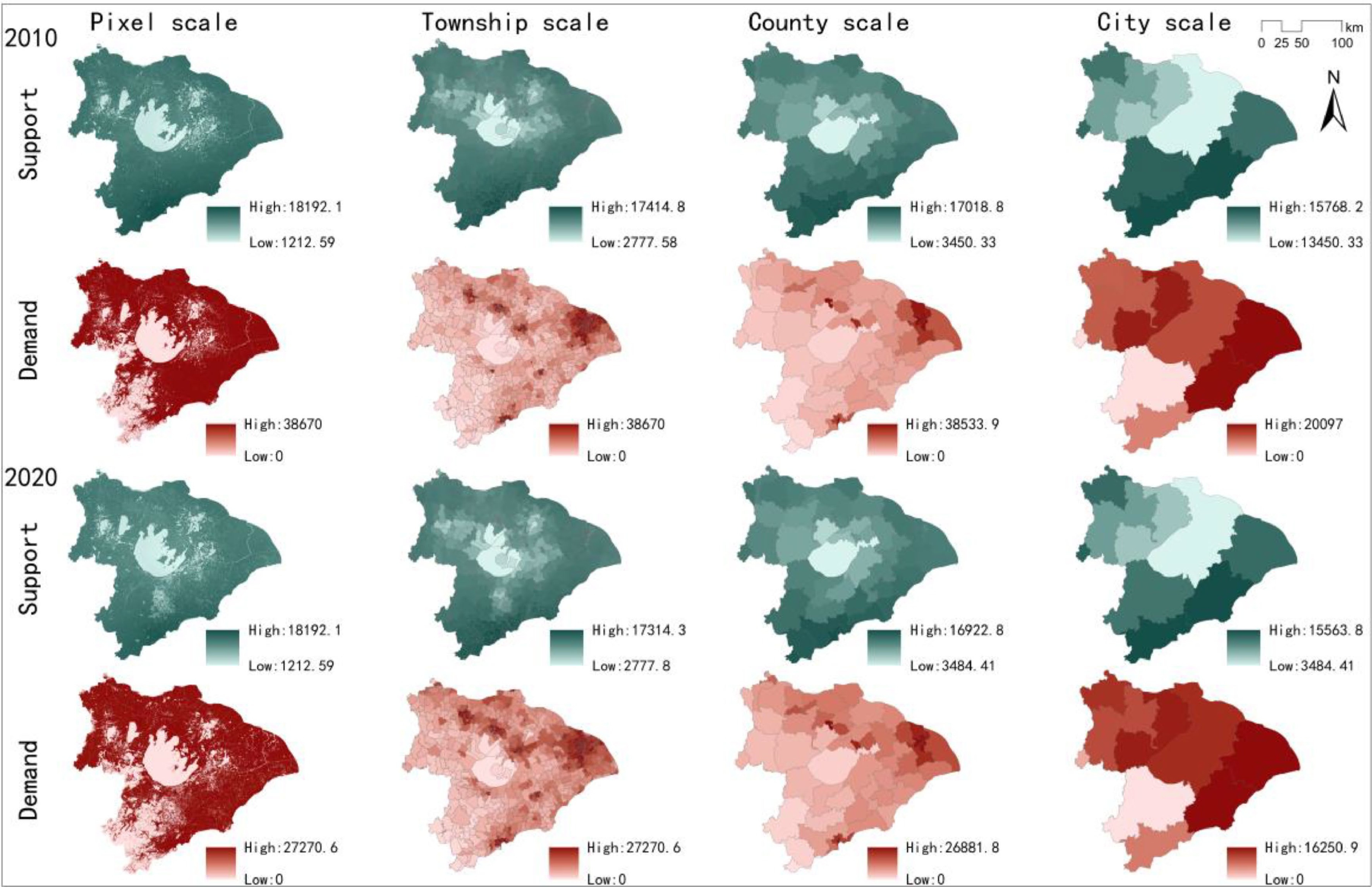
Figure 2. 

Spatial distribution of supply and demand of water yield service.

As shown in Fig. 3, the supply of water yield at the pixel scale is slightly higher than other scales, and the median supply at township, county, and city scales have little change. However, the demand for water yield is very low at the pixel scale. It increases rapidly at the township scale, and then it shows a downward trend with an increase in scale. Only the pixel scale and the township scale are correlated with the supply service. However, the correlation is not strong on other scales, and there is a strong correlation between the demand and service scales.

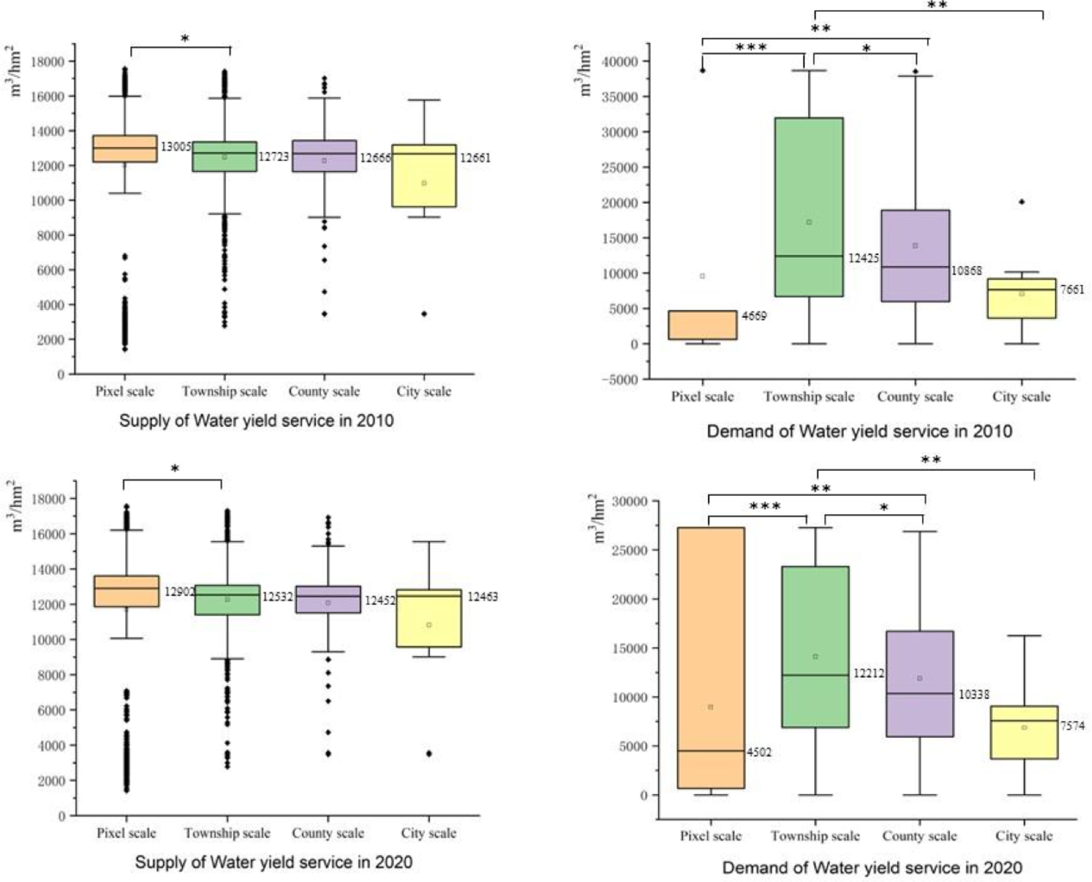
Figure 3. 

Maps showing water yield supply, demand, and correlation analysis. (When p < 0.05, it is marked with '*'. When p < 0.01, it is marked with '**'. When p < 0.001, it is marked with '***') in TLB in 2010 and 2020.

(2) Carbon sequestration service

In 2010, the total carbon sequestration supply was 0.14 billion tons, whereas the total carbon sequestration demand was 1.92 billion tons, and the gap between supply and demand was 1.79 billion tons. In 2020, the total carbon sequestration supply will be 0.13 billion tons, while the total carbon sequestration demand will be 2.53 billion tons, and the gap between supply and demand will be 2.40 billion tons.

As shown in Fig. 4, from 2010 to 2020, the areas with a high supply of carbon sequestration services were mainly concentrated in the forest areas in the southwest. The areas with high demand were mainly located in economically developed and densely populated areas in the east. The supply in the southwest increased slightly, but the demand in the east increased rapidly.

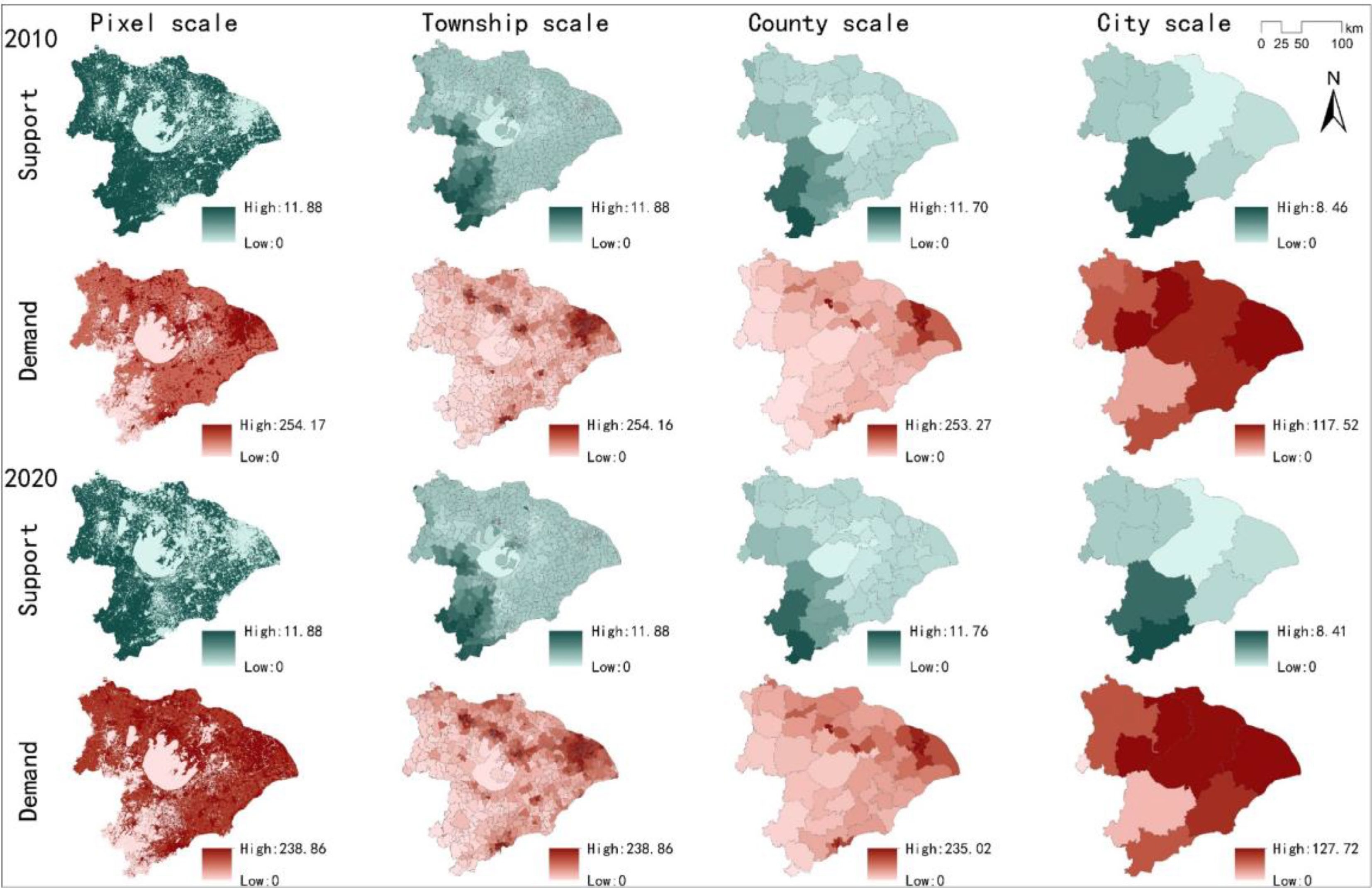
Figure 4. 

Spatial distribution of supply and demand of carbon sequestration service.

As shown in Fig. 5, the median supply of carbon sequestration services is consistent, except for the pixel scale, which shows a slightly increasing trend. The demand for carbon sequestration services is very low at the pixel scale before declining and increasing rapidly at the township scale and then shows a downward trend at an increasing scale. Only the pixel and the township scales are associated with the supply service. On the other scales, however, the correlation is weaker, although there is a strong correlation between the demand and service scales.

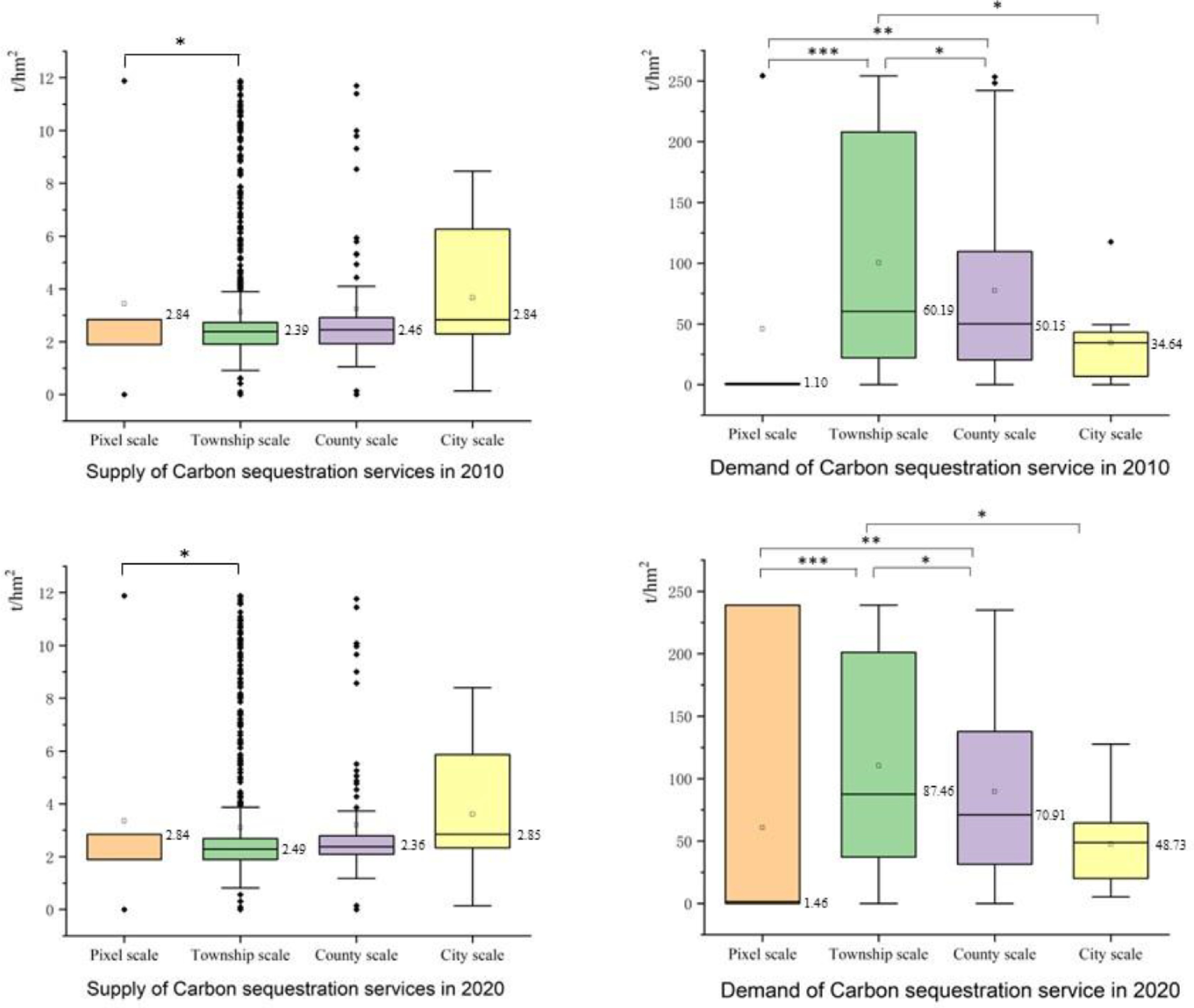
Figure 5. 

Maps showing carbon sequestration supply, demand, and correlation analysis. (When p < 0.05, it is marked with '*'. When p < 0.01, it is marked with '**'. When p < 0.001, and it is marked with '***') in TLB in 2010 and 2020.

(3) Recreation service

In 2010, the total supply of recreation was 6.07 million hm², while the total demand for recreation was 0.56 million hm², resulting in a surplus of 5.52 million hm². In 2020, the total supply of recreation will be 6.19 million hm², whereas the total demand will be 0.72 million hm², resulting in 5.47 million hm².

As shown in Fig. 6, from 2010 to 2020, the high supply areas for recreation services were in lakes and woodland areas in the central and southwest, and the high demand areas were in densely populated areas in the east. The supply of recreation services in the eastern region has decreased slightly, the demand has remained unchanged, and the overall supply and demand pattern has not changed much.

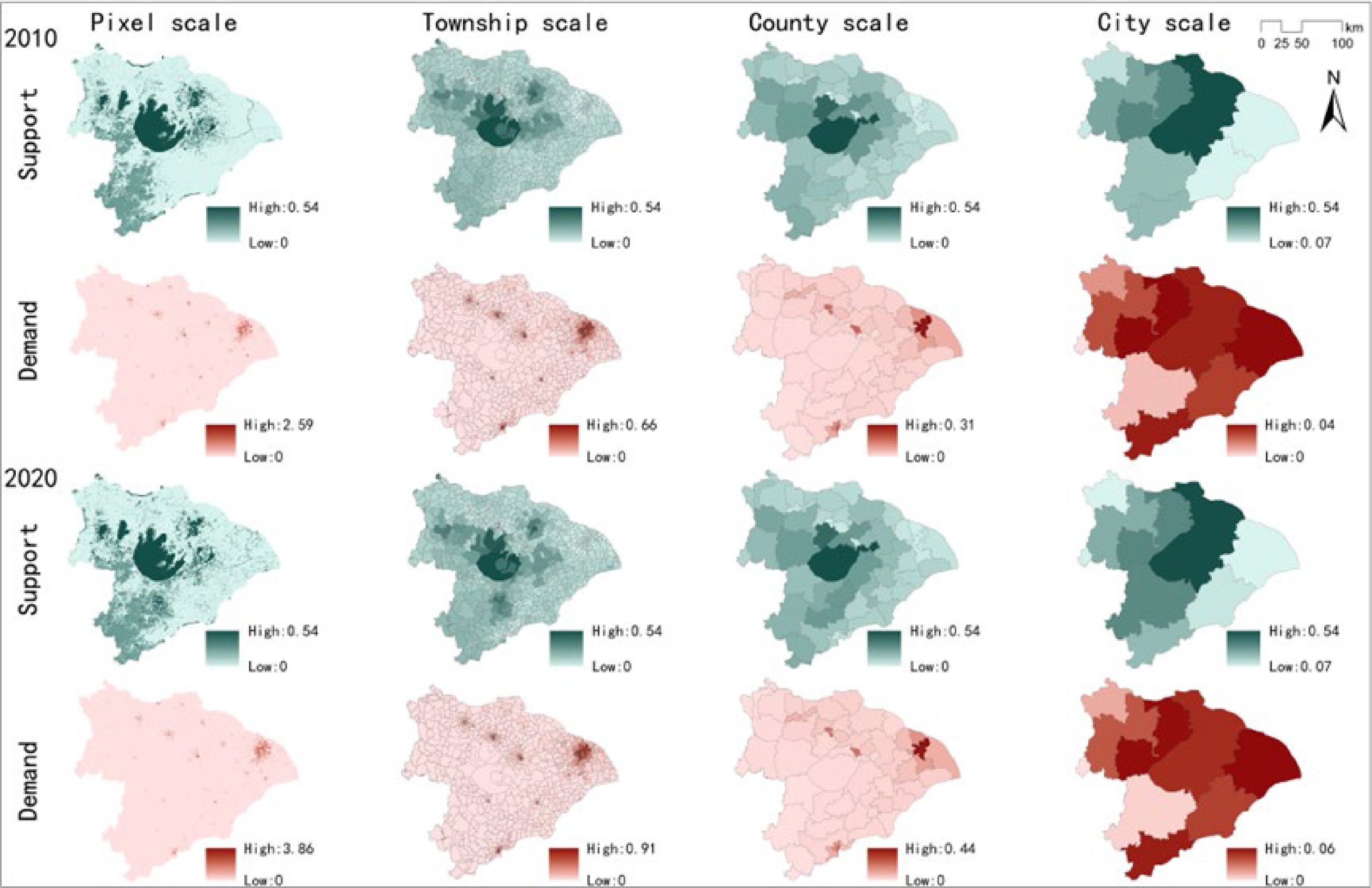
Figure 6. 

Spatial distribution of supply and demand of recreation service.

As shown in Fig. 7, the median supply of recreation services increases with the increase of scale. While the median demand decreases slightly with the increase of scale, and the overall change is not obvious. There is a correlation between the pixel scale and the township scale, the township scale, and the city scale, although it is not significant. However, there is a strong correlation between the demand and service scales.

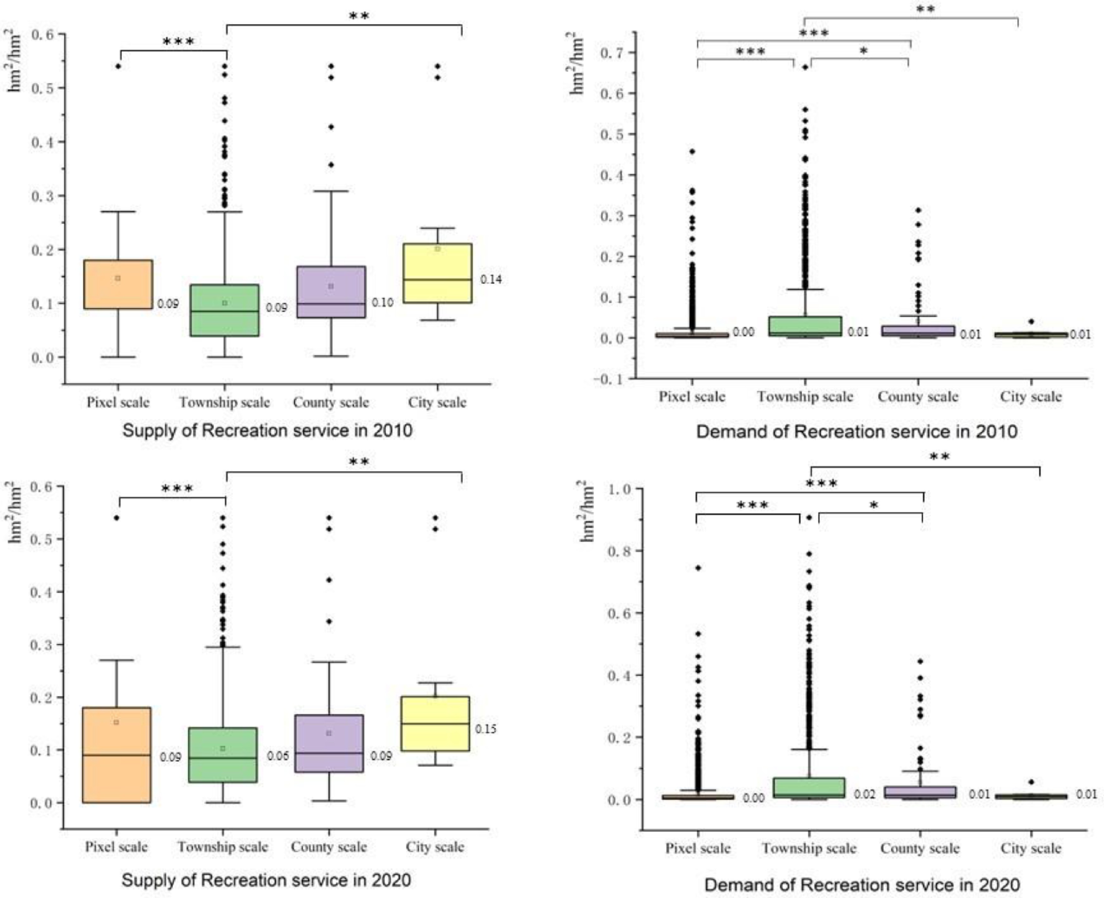
Figure 7. 

Maps showing recreation supply, demand, and correlation analysis. (When p < 0.05, it is marked with '*'. When p < 0.01, it is marked with '**'. When p < 0.001, it is marked with '***') in TLB in 2010 and 2020.

(4) Food production service

In 2010, the total food supply was 253 million tons, while the total food demand was 169 million tons, resulting in a surplus between supply and demand of 84 million tons. In 2020, the total food supply will be 234 million tons, while the total food demand will be 243 million tons, and the gap between supply and demand will be 9 million tons.

As shown in Fig. 8, from 2010 to 2020, the high food supply areas were mainly located in the cultivated land areas in the north and south. The high food demand areas were mainly located in the population concentrated regions in the east. Food supply services increased slightly in the northwest, decreased somewhat in the east, and food demand services increased slightly in the east and south. However, the overall supply and demand pattern did not change much.

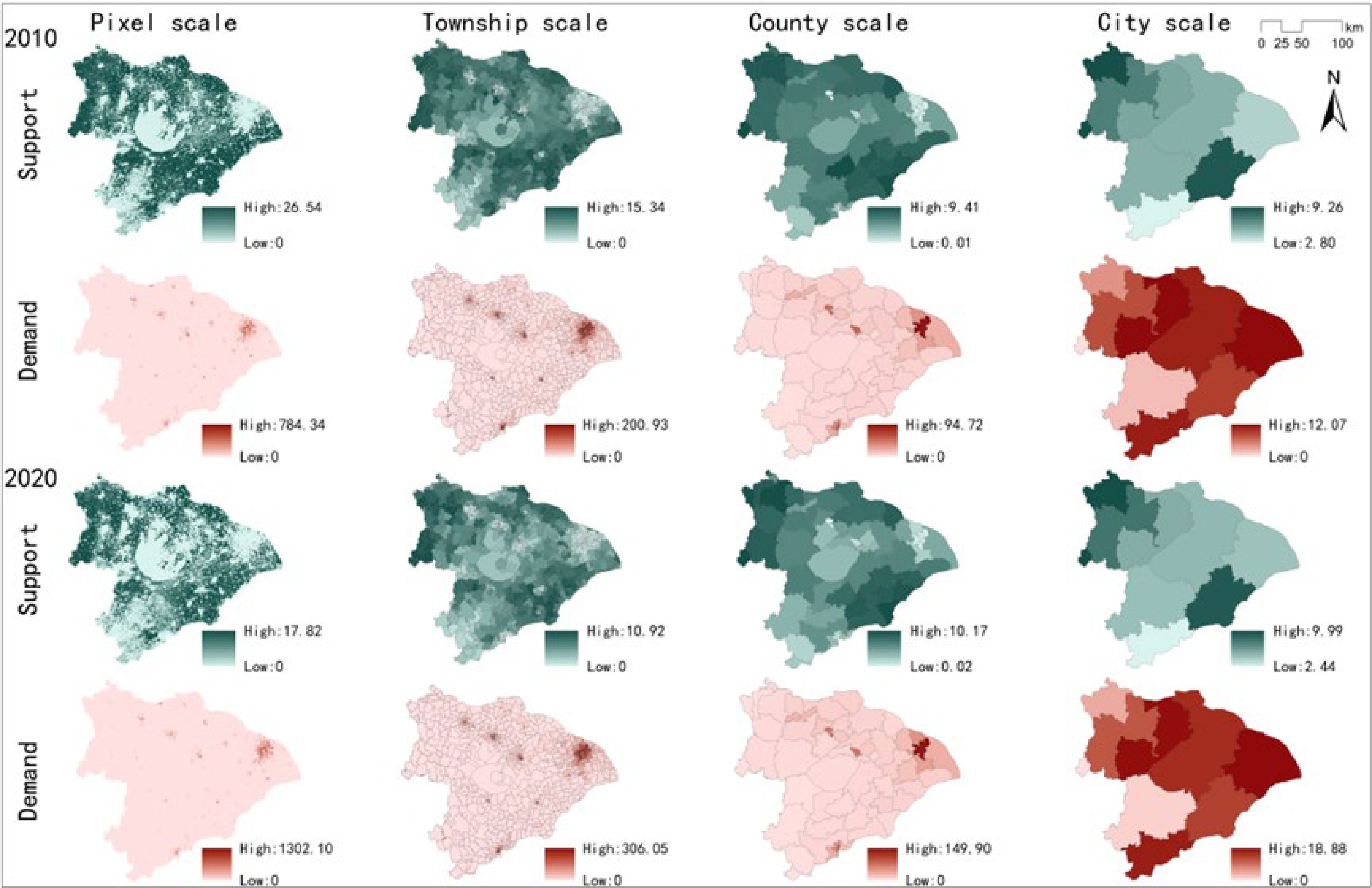
Figure 8. 

Spatial distribution of supply and demand of food production service.

As shown in Fig. 9, in addition to the higher median supply of food production at the pixel scale in 2010, the median supply of food at other scales also increases with the increase of scale. In addition to the pixel scale, the average demand for food production decreases with an increase in scale. Only the pixel scale and the township scale are correlated with supply service. However, the correlation is not strong on other scales, and there is a strong correlation between the demand and service scales.

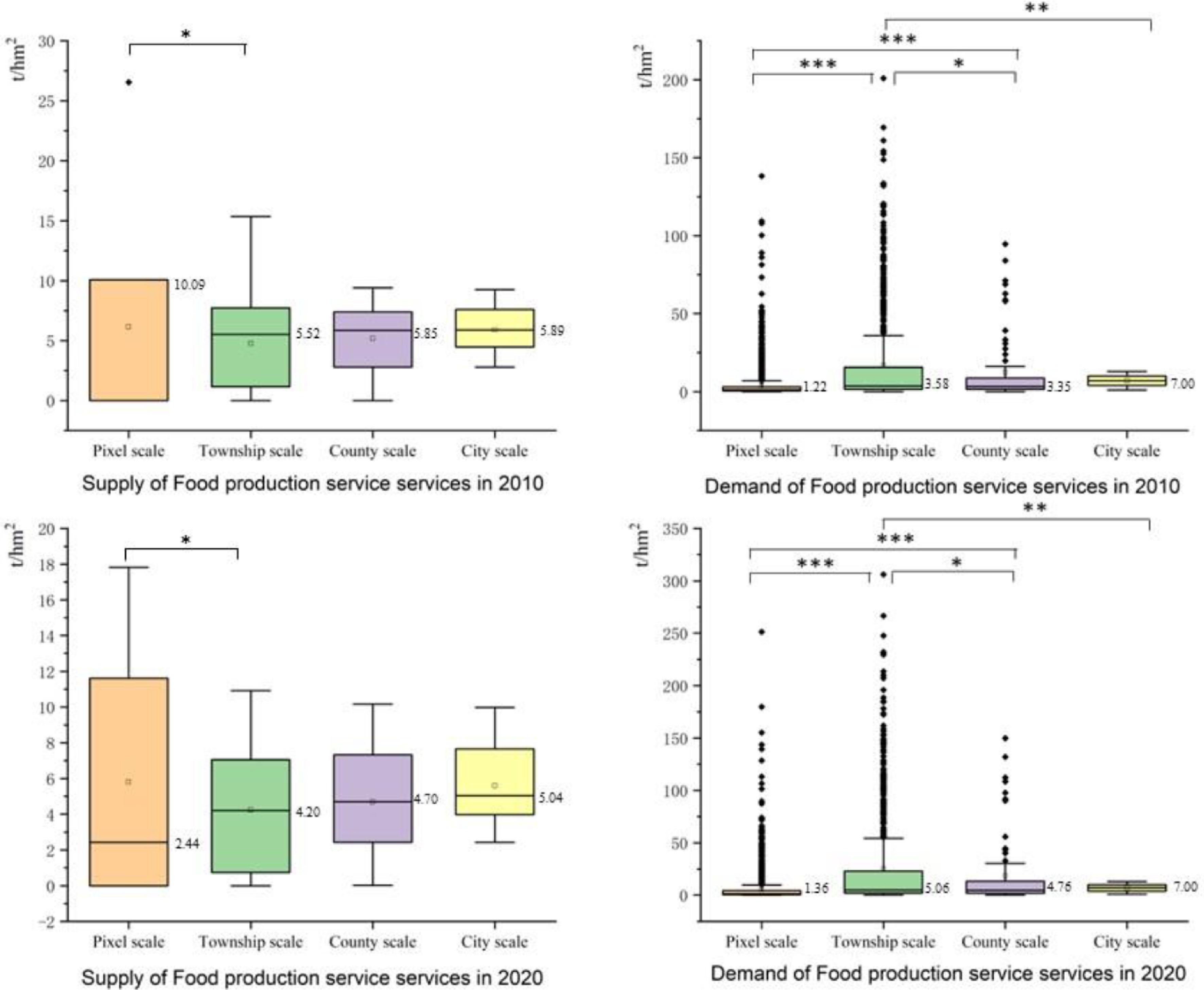
Figure 9. 

Maps showing food production supply, demand, and correlation analysis. (When p < 0.05, it is marked with '*'. When p < 0.01, it is marked with '**'. When p < 0.001, it is marked with '***') in TLB in 2010 and 2020.

(5) Heat regulation service

In 2010, the average supply of heat regulation was −1.02 °C, while the average demand for heat regulation was 0.03 °C, resulting in an average gap between supply and demand of −1.05 °C. In 2020, the average supply of heat regulation will be −4.84 °C, the average demand for heat regulation will be 0.03 °C, and the average gap between supply and demand will be −4.87 °C.

As shown in Fig. 10, from 2010 to 2020, the high supply of heat regulation services in TLB were mainly distributed in lakes, wetlands, and woodland areas in the middle and south. The high demand areas were primarily located in densely populated areas in the east. The supply of heat regulation in most areas in the north and south shows a downward trend, while the demand for heat regulation in counties in the middle, south, and northwest is increasing.

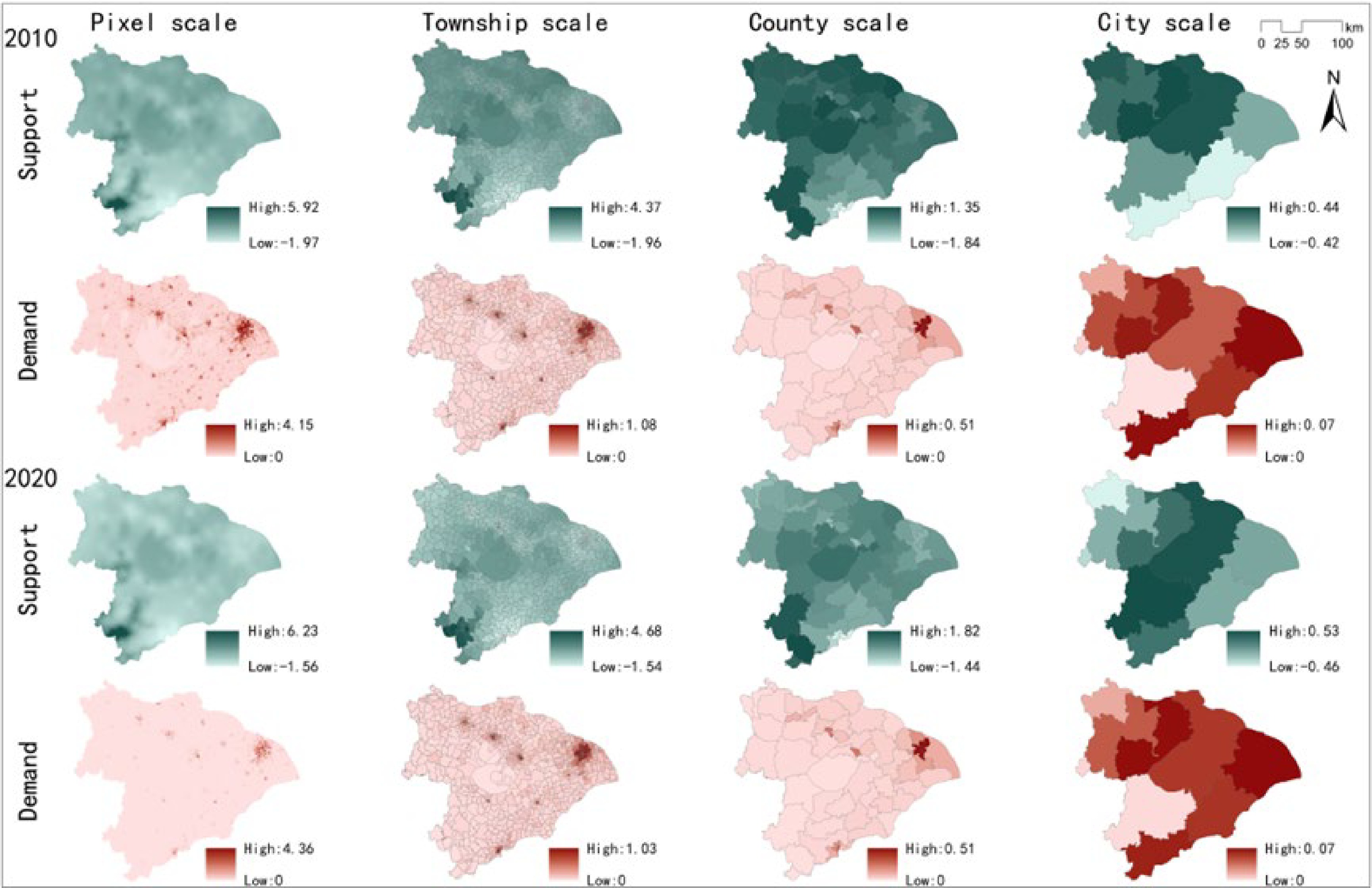
Figure 10. 

Spatial distribution of supply and demand of heat regulation service.

As shown in Fig. 11, except for the pixel and city scales in 2010, the median value of the supply service of heat regulation is positive and less than 0.1 at all other scales. In addition to the pixel scale, the median amount of heat regulation increases with the increase in scale. The demand for heat regulation decreases slightly with an increase in scale, but the median demand changes little as a whole. Only the pixel scale and township scale, pixel scale, and county scale correspond strongly, but the association between demand service scales is substantial at all levels.

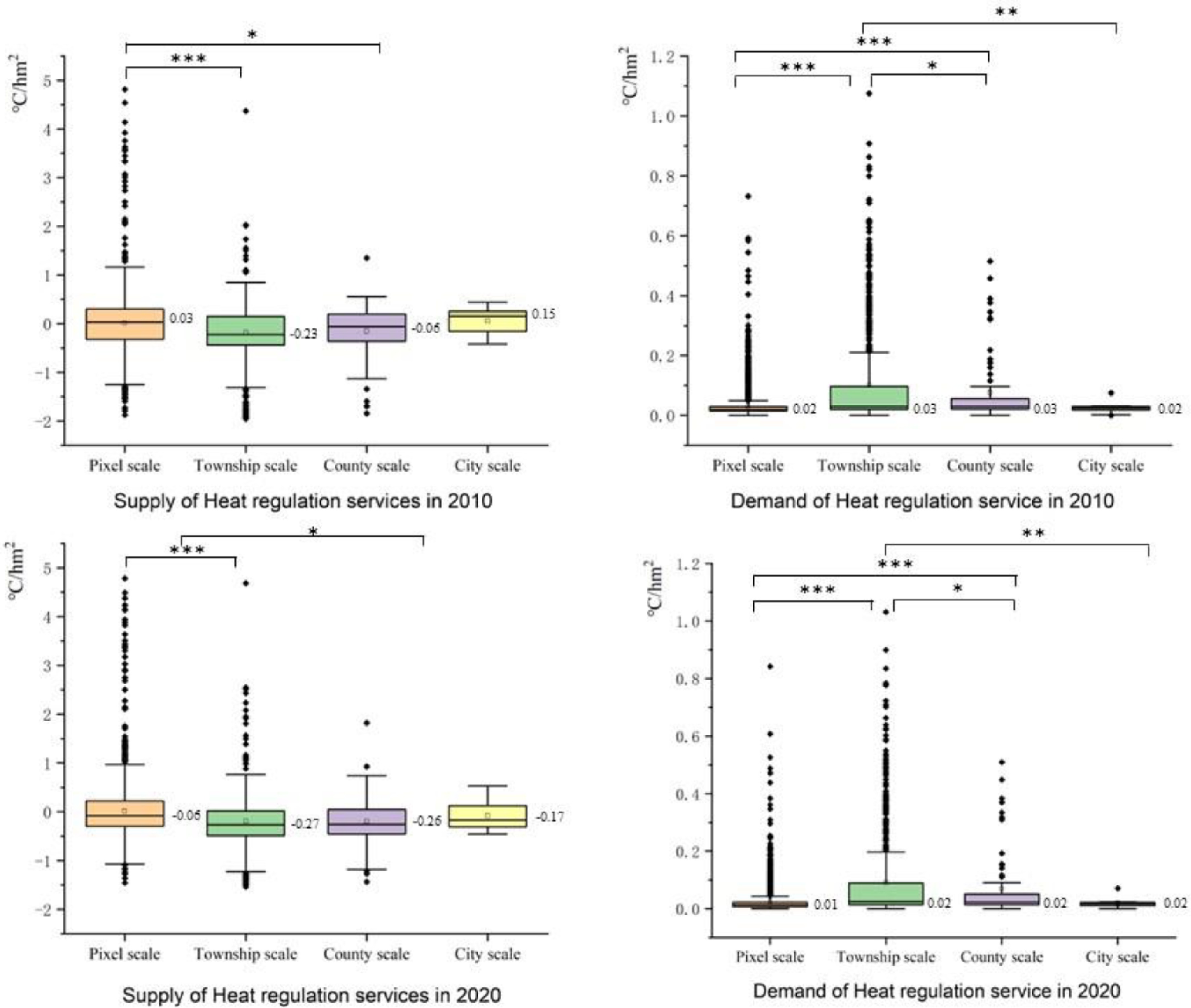
Figure 11. 

Maps showing heat regulation supply, demand, and correlation analysis. (When p < 0.05, it is marked with '*'. When p < 0.01, it is marked with '**'. When p < 0.001, and it is marked with '***') in TLB in 2010 and 2020.

Spatial distribution, quantity difference, scale feature and matching characteristics of ESDR

(1) Water yield service

From 2010 to 2020, the high deficit areas of water yield services are mainly located in the eastern and central urban areas. In contrast, the high surplus areas are mainly found in forest land in the southwest. Although the water yield services of villages and towns in TLB's eastern, northern, and central regions are decreasing, the spatial pattern of high surplus and the high deficiency remains unchanged.

As shown in Fig. 12, in 2010, the average ESDR of water yield services in TLB was 0.05, but by 2020, it had increased to 0.11, indicating that the water yield services in TLB were slightly surplus, and the surplus was increasing. The median of each scale is greater than 0. Except for the pixel scale, the scale of towns, counties, and cities increased progressively between 2010 and 2020, and there was a correlation between all scales.

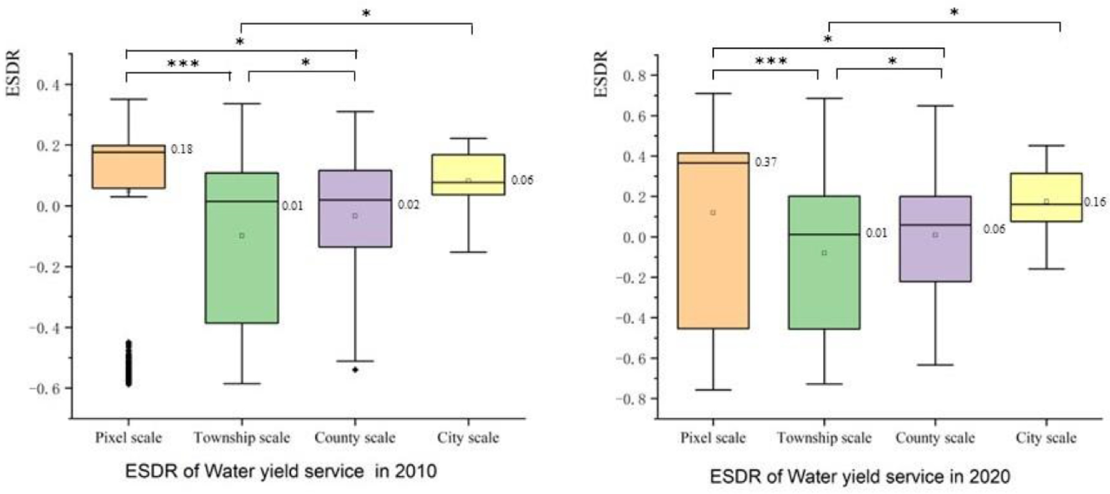
Figure 12. 

ESDR of water yield service under different scales and correlation analysis. (When p < 0.05, it is marked with '*'. When p < 0.01, it is marked with '**'. When p < 0.001, and it is marked with '***') in TLB in 2010 and 2020.

(2) Carbon sequestration service

From 2010 to 2020, the highest deficit areas for carbon sequestration services were mainly in densely populated and economically developed areas in the east and middle. The largest surplus areas were mainly located in woodland in the southwest. Carbon sequestration services in some towns and villages in the eastern region changed from balance to deficit or high deficit. However, in some areas in the eastern and southern regions, from balance to surplus.

As shown in Fig. 13, the ESDR for carbon sequestration services in 2010 and 2020 were −0.33 and −0.47, respectively, and the carbon sequestration services revealed a slight deficit that was still deepening. The median of the pixel scale is greater than 0, rapidly decreasing to a negative number on the township scale, and the median of township, county, and city scales is less than 0, and all of them show a gradual upward trend.

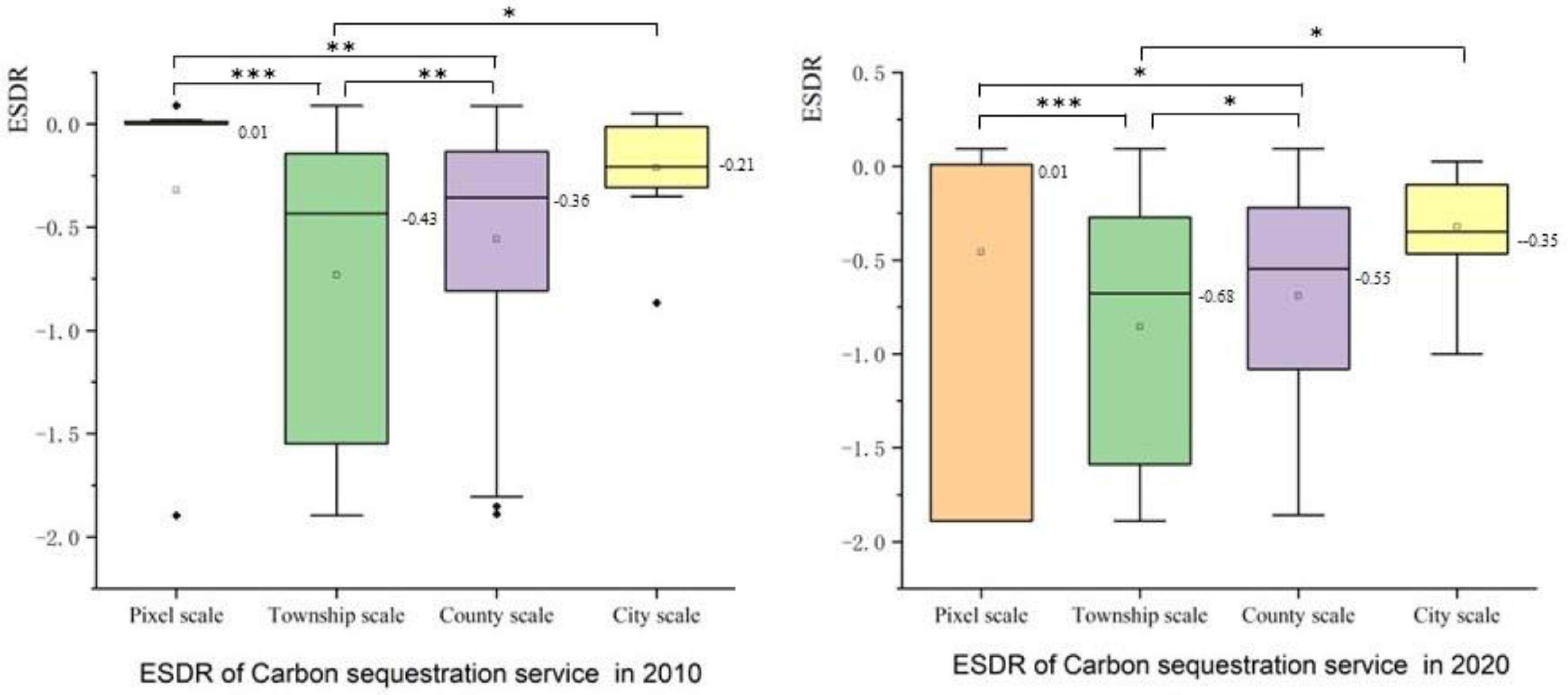
Figure 13. 

ESDR of carbon sequestration service under different scales and correlation analysis. (When p < 0.05, it is marked with '*'. When p < 0.01, it is marked with '**'. When p < 0.001, it is marked with '***') in TLB in 2010 and 2020.

(3) Recreation service

In 2010 and 2020, the high surplus of recreation services was mainly in the central region around TLB, while the high deficit region was mainly in the eastern region. Towns with large surplus and recreation services deficits remain unchanged, but some surplus areas become balanced. There is no change in the spatial pattern of supply and demand at the county and city scales.

As shown in Fig. 14, ESDR of recreation services in 2010 and 2020 are 0.09 and 0.06. Although recreation services are still in surplus, the surplus is decreasing. In addition to the pixel scale, the median of township, county, and city scales all showed an increasing trend, but the numerical increase was small.

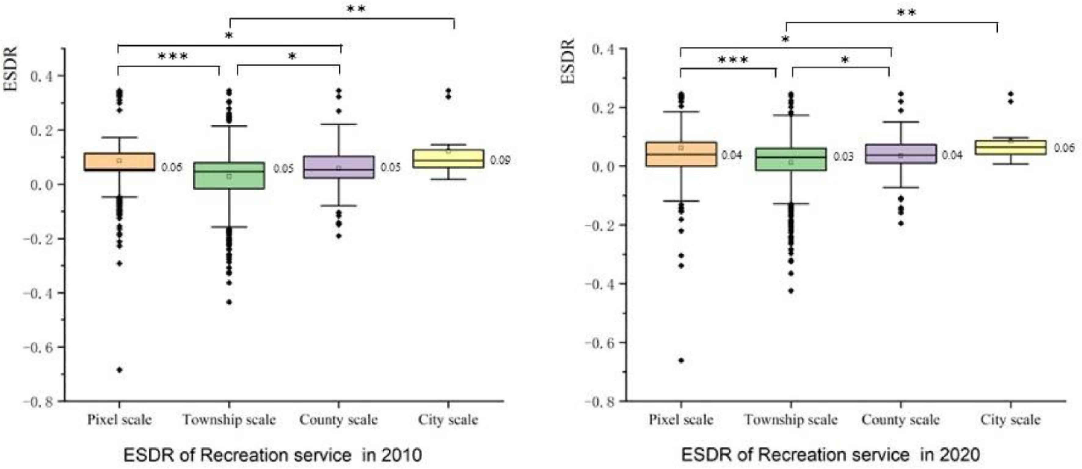
Figure 14. 

ESDR of recreation service under different scales and correlation analysis. (When p < 0.05, it is marked with '*'. When p < 0.01, it is marked with '**'. When p < 0.001, and it is marked with '***') in TLB in 2010 and 2020.

(4) Food production service

From 2010 to 2020, most of the areas with a high food production service deficit were in the east, with a large population and a strong economy. The areas with increased food production and service surplus are mainly located on cultivated land in the northwest and south. Overall, the spatial pattern of food production service has not changed much.

As shown in Fig. 15, the food production service changed from 0.01 to −0.01 and from a slight surplus to a slight deficit. The median values on all scales are close to 0. Except for the pixel scale, the median values on township, county, and city scales have increased, but the numerical increase is very small.

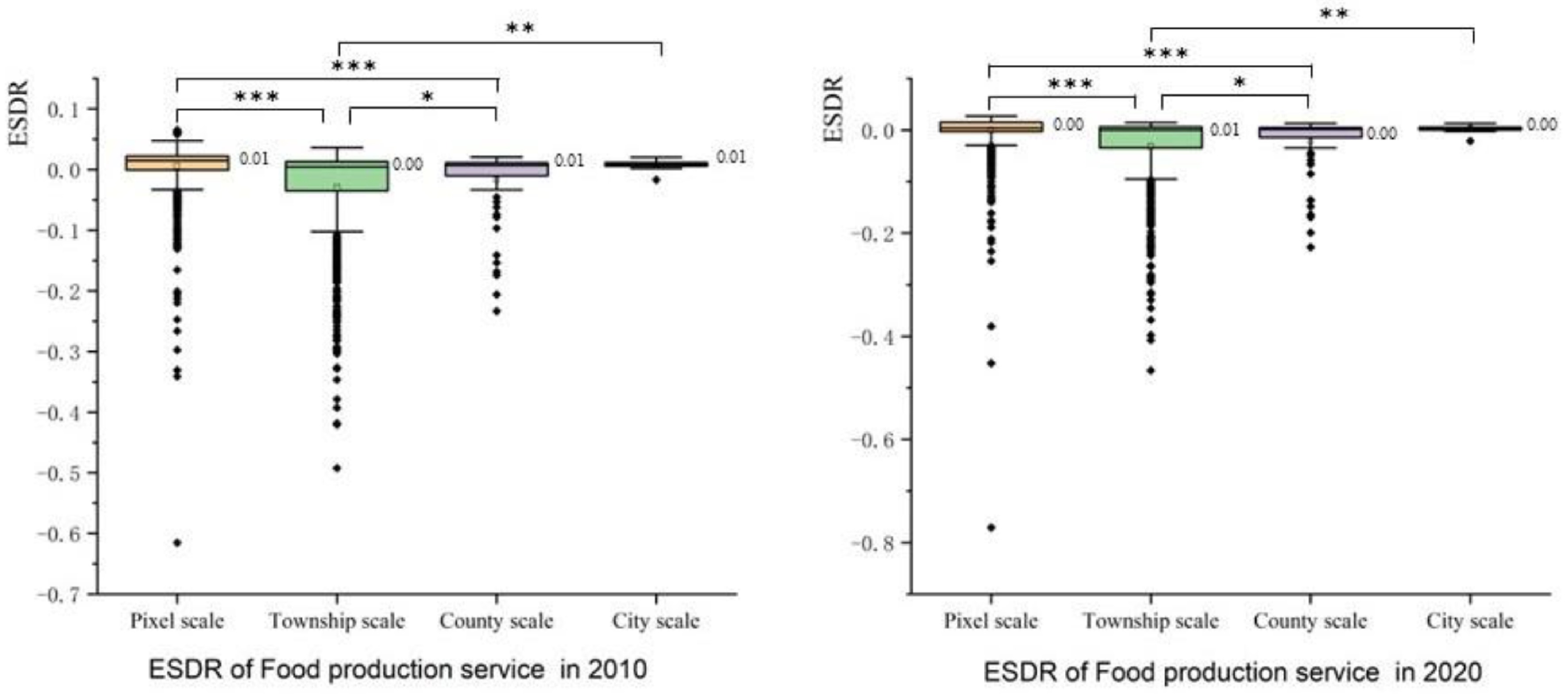
Figure 15. 

ESDR of food production service under different scales and correlation analysis. (When p < 0.05, it is marked with '*'. When p < 0.01, it is marked with '**'. When p < 0.001, and it is marked with '***') in TLB in 2010 and 2020.

(5) Heat regulation service

In 2010, the high deficit area of heat regulation service was mainly in the central and southern regions. In 2020, the increased deficit area was mainly in the northwest. High surplus areas are distributed in a small number of woodlands in the southwest.

As shown in Fig. 16, the heat regulation service has changed from −0.006 to −0.005, and the overall heat regulation service is still in a deficit state, and the deficit degree is slightly reduced. Except for the median values of pixel scale and city scale in 2010, the median values of other scales and years are less than 0. Except for the pixel scale, the median of the heat regulation service ESDR increases with scale. The ESDR of heat regulation service has a strong correlation only between pixel scale and county scale, pixel scale and city scale, and other scales are not strong. Spatial distribution of ESDR at different scales as shown in Figs. 17 and 18.

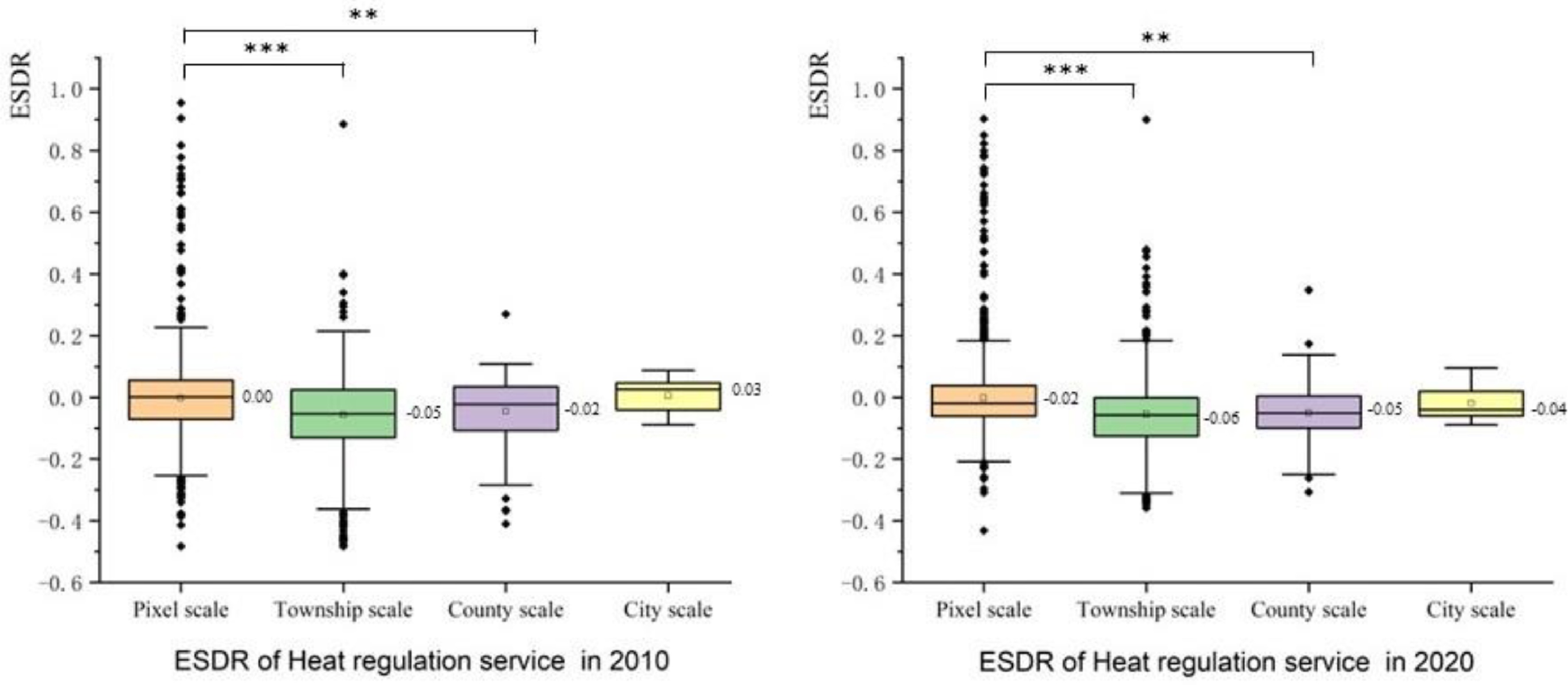
Figure 16. 

ESDR of heat regulation service under different scales and correlation analysis. (When p < 0.05, it is marked with '*'. When p < 0.01, it is marked with '**'. When p < 0.001, and it is marked with '***') in TLB in 2010 and 2020.

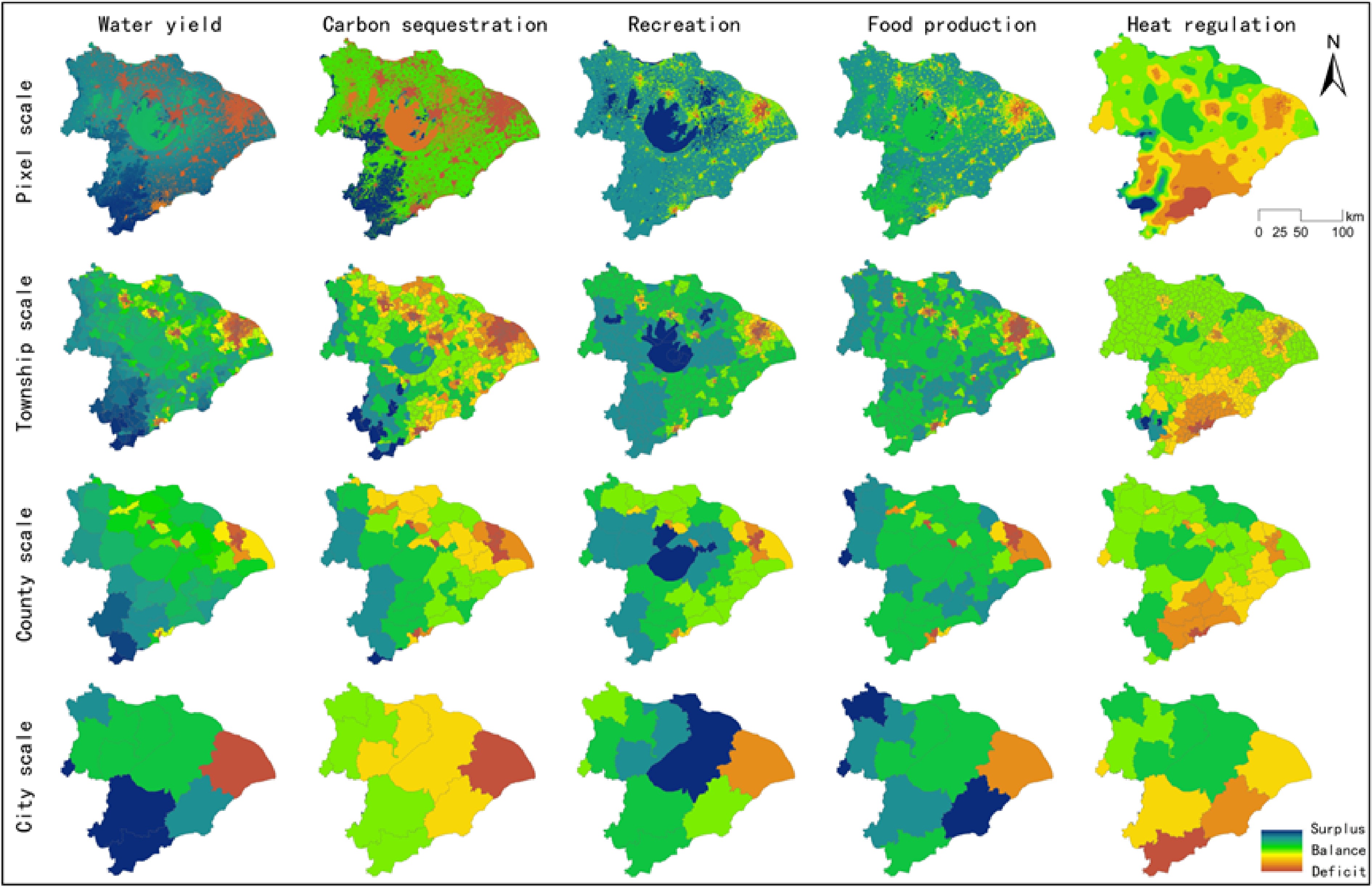
Figure 17. 

Spatial distribution of ESDR at different scales in 2010.

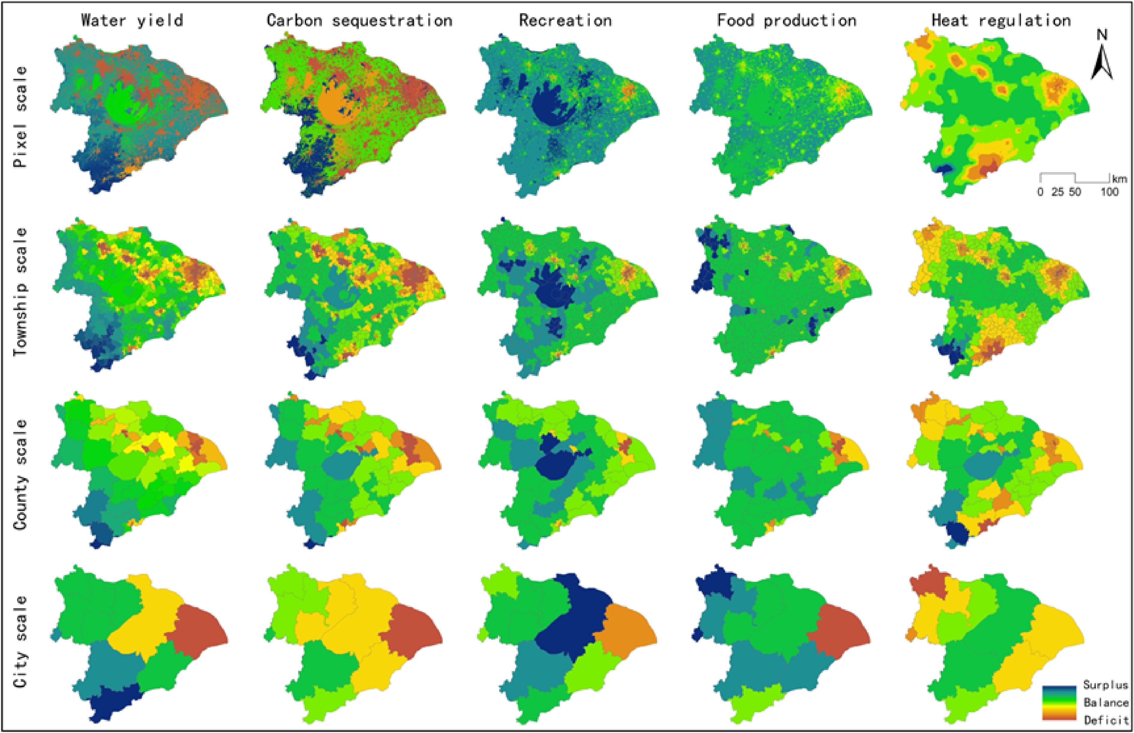
Figure 18. 

Spatial distribution of ESDR at different scales in 2020.

Spatial distribution, quantitative characteristics, and matching of the CESDR

As shown in Figs. 19 and 20, in 2010, the average value of CESDR in TLB was −0.03; in 2020, it was −0.05, and the overall value of CESDR showed a downward trend. In addition to the pixel scale, the median increases as the research scale increases. Among them, the median number on the pixel scale is greater than 0, while the median values on other scales are less than 0. In 2010, the correlation between each scale was strong, but the correlation between the county and city scales was not strong in 2020.

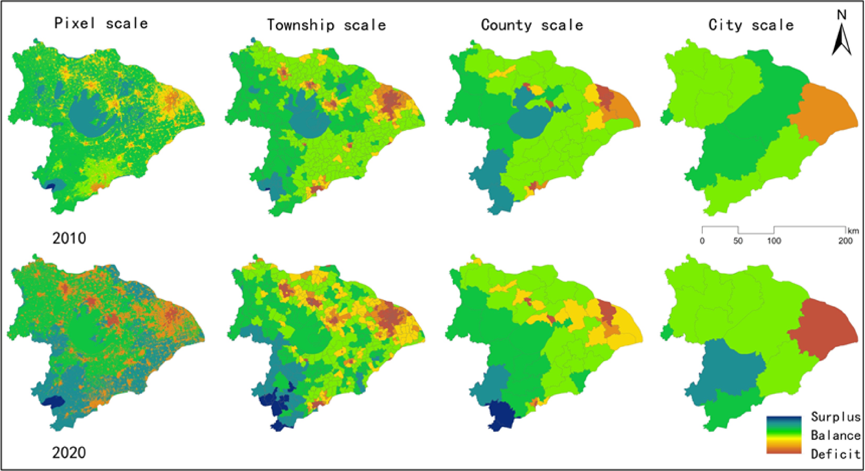
Figure 19. 

Spatial distribution of CESDR at different scales.

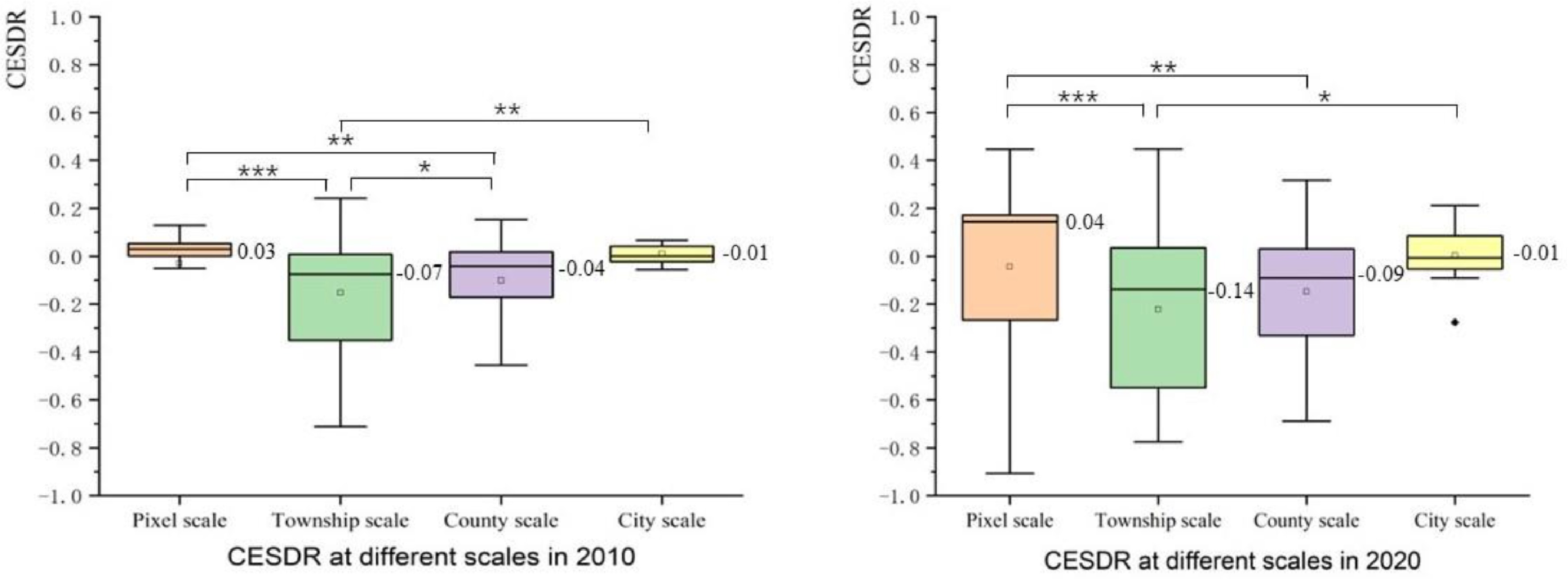
Figure 20. 

CESDR under different scales and correlation analysis. (When p < 0.05, it is marked with '*'. When p < 0.01, it is marked with '**'. When p < 0.001, it is marked with '***') in TLB in 2010 and 2020.

As shown in Fig. 19, the southern and western regions of TLB provide more resources and services than their own needs, resulting in surpluses. Moreover, the surpluses generated by each administrative region vary, and there are certain spatial differences. The southwest region has the largest surplus and is classified as a high surplus region. The urbanized areas in the east, middle, and south are severely underserved. The area in the east that requires replenishment by supply services is increasing. In addition, the number of deficits is also increasing, which aggravates the problem of resource shortages. The main areas of the imbalance between the supply and demand of ESs in TLB, according to the scale of urban management, are concentrated in the main districts and counties of Shanghai, Suzhou, Wuxi, and other big cities spreading from the core towns to the outside.

As shown in Table 2, we conducted variance tests on CESDR at different scales in TLB in 2010 and 2020. The results of the variance test show that in 2010, except for pixel scale and city scale, county scale, and urban scale, the other scales in the TLB are p > 0.05, meeting the standard requirements. In 2020, except that the pixel scale and urban scale, county scale and township scale, and county scale and urban scale are not significant, other scales were p > 0.05, meeting the standard requirements.

As ESs include both supply and demand, it is necessary to combine the two aspects of analysis and consider supply and demand synthetically when making policy suggestions to improve the deficits of different ESs^[17]. From the quantitative perspective, the overall supply of TLB ESs showed a slight decline from 2010 to 2020. The demand for TLB is increasing rapidly, especially in urban centers and surrounding towns in the eastern and central areas of the basin. From the perspective of spatial pattern, the distribution pattern of supply and demand services in 2010 and 2020 has not changed significantly. The high supply area of water yield and carbon sequestration services is mainly located in the forest land in the southwest of the TLB, and the high supply area of recreation and heat regulation services is mainly located in the central water body and wetland area of the TLB, and the high supply area of food production services is mainly located in the northern and southern arable land. The high demand areas for the five service types are mainly located in urban areas in the eastern and central regions. These areas generally have high energy consuming industries and urban construction activities with enormous demands.

ESDR and CESDR of different types of TLB ESs in 2010 and 2020 are both less than 0, indicating that TLB ESs have deficits. From the analysis of the matching results of supply and demand for ESs, it can be seen that the TLB area has been rapidly urbanized over the past decade and that the quantity and spatial differences between supply and demand for ESs have been increasing, with the contradiction between supply and demand for carbon sequestration services and heat regulation services being the most prominent, which has become a significant factor that severely limits the development of ESs. At the same time, there is a certain demand gap for water yield services and food production services. Although recreation services were still in surplus in 2020, their ESDR rapidly declined. The research results of this part of the supply and demand pattern are the same as those of previous studies on the supply and demand pattern of TLB and its surrounding areas^[41]. Compared with previous research on ecosystem services in the TLB^{[9, 41, 43, 50]}, the spatial pattern of water yield, carbon sequestration, recreation, and food production services at the pixel scale is the same as that of previous research, and heat regulation services are greatly affected by climate change. Because the flow of supply and demand on different time and space scales is very complicated, it is relatively difficult to find clear and definite indicators to describe this relationship^[27]. The pixel scale is analyzed by extracting data from random points. No matter the overall spatial pattern of TLB in 2010 or 2020, the surplus area is larger than the deficit area. This results in a higher median pixel scale and more random points in the surplus area. This shows that although the serious deficit area only occupies a small area, it plays an imperative role in the overall ecosystem service of TLB. It also has a significant impact. The supply of water yield, carbon sequestration, and heat regulation services is mainly affected by the natural environment. Therefore, the supply of these three services is less affected by the administrative scale, and the correlation between the scales is not strong. However, the demand is primarily influenced by the social economy, and the demand in densely populated and economically developed regions is substantial. Thus it is also greatly influenced by the administrative scale, with a strong correlation between the scales.

The existing research findings show that with the continuous increase in spatial scale, the spatial matching of ESs has gradually changed^[37]. Through CESDR's evaluation of the matching degree of supply and demand of ESs of different scales in 2010 and 2020, we found that in the two years, the cities and towns with serious supply and demand mismatches were the areas where people gathered. Because of the developed economy, these towns attract a large number of people to gather, which makes the urban built-up area expand continuously and encroaches on a large amount of original ecological land area. However, these seriously mismatched areas cannot achieve effective ecological control, so the supply and demand of ESs in the surrounding areas are out of alignment. This leads to mismatches on a larger district and county scale, where ESs continue to deteriorate, and mismatches on a city scale, eventually lead to ESs mismatch in the whole region. With the increase in research scale, the median value of TLB in 2010 and 2020 gradually decreased. This is mainly due to the allocation of ESs resources that are allocated at different scales, alleviating the mismatch between supply and demand in areas with serious deficits. The study of supply and demand at the scale of cities and counties cannot sufficiently express the quantitative relationship However, it can intuitively show the spatial pattern of the whole ESs.

Management implications

This paper attempts to analyze the quantitative characteristics and spatial-temporal pattern of the relationship between the supply and demand of ESs in TLB at different scales. Furthermore, it reveals the matching characteristics and spatial distribution law of different services. Afterward, it integrates the research results at the pixel scale with administrative divisions to determine the benefits range and flow of services so that decision-makers can better manage resources. In this regard, we make the following suggestions.

Firstly, we suggested that scale characteristics should be incorporated into ecosystem management decisions. Multi-scale analysis can not only reflect the fine situation of small scale^[38] but also reflect the spatial pattern of large scale. It can better help the decision-making and management of ESs^[51]. No matter whether in 2010 or 2020, most ESs indicators increase with the increase of spatial scope, but their scale relationship is different^{[27, 28]}. The data collection and analysis process is restricted by government statistical information and spatial resolution. In the process of scale aggregation and decomposition, the results of small scales, such as pixel scale and township scale, can be well aggregated into large scale data, while the effects of urban scale data are not accurate when decomposed into small scale^[52]. Therefore, government departments should be encouraged to collect as much information as possible in order to better analyze at different scales^[30].

Secondly, we suggested that the balance between supply and demand can be achieved through reasonable ecological protection and restoration. The southwest region with high forest coverage and a good natural environment provides high services, while the eastern and central regions with dense populations and rapid urban expansion have a large demand for ESs. Therefore, ecological protection and development of ecological resources should be continuously strengthened in areas with high supply in the southwest of the TLB, and ecological construction and restoration should be emphasized in areas with high demand in the east^{[41, 53]}. The supply and demand mismatch in the eastern, central, and other local areas will affect the overall supply and demand balance in the TLB. Therefore, it is necessary to alleviate the supply and demand contradiction in local areas. It is necessary to coordinate the spatial management and control of land use in river basins, better carry out land planning and management, optimize the spatial structure, realize the spatial synergy between spatial land development and ecological environment constraints, and further alleviate or offset the ESs mismatch^[54]. Especially for carbon sequestration services and heat regulation services, the contradiction between supply and demand is prominent. It is necessary to adjust industrial structures, reduce carbon emissions, improve vegetation coverage in densely populated areas, and pay attention to climate change.

Thirdly, we suggest strengthening the analysis of ESs flows and stakeholders. Policy formulation and management should be considered comprehensively and should conform to the actual situation of the ecosystem managed at each administrative level. Considering the different spatial development differences in the basin, different regions can explore comprehensive development models suitable for their own coordinated economic, social, and natural development^[2]. Multi-regional, and multi-scale linkage makes the carrying capacity of resources and environment in the region coordinate with the development level. The actual influence scope of most ESs is beyond the administrative boundary. Therefore, policymakers should incorporate the actual scope of ESs into sustainable development planning, not just rely on the administrative boundary^{[55, 56]}.

Limitations and prospects for future perspectives

Although our method evaluates the supply and demand for ESs at different scales, it has some limitations. Data collection and analysis are constrained by statistical information and spatial resolution. Multi-temporal dynamic ecosystem supply and demand changes may be more beneficial to policymakers or understanding regional supply and demand adjustment^[54]. However, this study did not fully consider this point because it only selected two years to compare supply and demand changes. During this research, we only considered the TLB and did not assess the larger area. However, both the providers and beneficiaries of ESs differ in time and space. For example, the supply of carbon sequestration and heat regulation services is in the TLB, but its beneficiaries are outside the basin. This convenient development of transportation and market oriented transactions has also increased the difficulty of evaluating services^[57]. For recreation services, we compare the supply and demand of green space as a service. However, other facilities can also provide recreation services, which we have not fully considered. Although the supply and demand of all services can be considered comprehensively by introducing CESDR, each service type is different. It is impossible to confirm which service type has the most significant influence by a comprehensive consideration of the ratio.

In this research, only the types of land use that can provide services to people are calculated. Land characteristics of different land use types, such as biomass, species richness, landscape size, and shape, are not considered, which could affect ESs. On the demand side, different land landscapes, income levels, education levels, customs, etc., will also affect the demand for services, and these influencing factors are not taken into account. The analysis of the supply and demand drivers in the TLB can be more helpful to understand ESs, and the analysis of the drivers can be increased in the future. At the same time, since the frequency of human arrival decreases as the distance increases, and the assessment of ESs does not take into account the distance between residents and areas with high value of service supply, it is more accurate to explain the service decline pattern by applying marginal effects to describe the distance of residents to ecological land. The research on the source flow sink of ESs will also help us to realize cross regional resource allocation and alleviate the contradiction of supply and demand being at conflict.

Taking TLB as an example, this study quantified the supply and demand of five ESs, namely water yield, carbon sequestration, recreation, food production, and heat regulation services, at pixel scale, township scale, county scale, and city scale in 2010 and 2020. Then it investigated the mismatch between the supply and demand of ESs at different scales. According to the supply and demand balance characteristics, the quantitative relationship characteristics and spatial distribution patterns at different scales were graphically expressed. We found that the CESDR of TLB decreased from −0.03 to −0.05 from 2010 to 2020. The majority of high deficit areas were concentrated in densely populated urban centers and urbanized towns in the eastern and middle of TLB. In the meantime, the high surplus areas were mainly concentrated in the woodlands southwest of TLB. The deficit range of urban areas in the eastern and central regions is expanding, while the high surplus range in the southwest is decreasing. At the same time, the balance between supply and demand in 2010 is shifting towards deficit.

For different types of ESs, the scale of ESs is constantly changing. Fine scale research helps demonstrate spatial relationships and quantitative differences, whereas large scale research makes it easier to comprehend the spatial pattern of regional ESs, which is more accurate and makes the quantification and visualization of ESs easier to understand. The serious mismatch between supply and demand on a small scale will seriously affect the relationship between supply and demand on a larger scale. An increase in scale can also alleviate the contradiction between supply and demand on a small scale. We recommend that decision makers and managers incorporate scale analysis into ecosystem management decisions. Government departments should be encouraged to collect as much information as possible in order to better analyze at different scales. Realize the balance between supply and demand through reasonable ecological protection and ecological restoration. Strengthen the analysis of ESs flow and stakeholders. Therefore, research on the scale helps policymakers and managers select the appropriate scale effect. In addition, it helps them with convergence and coordination between scales in order to achieve a more efficient flow of ESs.