An improved particle swarm optimization algorithm based urban rail passenger flow prediction model: a case study in Beijing, China

Recently, unprecedented data availability and rapid development of machine learning techniques have led to tremendous progress in the intelligent transportation systems field^[1]. Accurate rail transit passenger flow prediction, as a prerequisite for real-time traffic signal control, traffic allocation, path guidance, automatic navigation, and determination of residential travel connection schemes in intelligent transportation systems, is currently a research hotspot in the transportation field^[2]. With the continuous development of urban rail transit systems in China, the diversification of passenger flow data sources and the massive scale of data, such as Automatic Fare Collection (AFC) system data, smart card data, and mobile phone signaling data, provide a data foundation for precise passenger flow prediction in rail transit. However, the passenger flow in urban rail transit is characterized by non-linearity, non-stationarity, and randomness, and is influenced by various internal and external factors, making accurate prediction challenging. Therefore, with the wide application of big data, artificial intelligence, cloud computing, and other emerging technologies in the field of rail transit, it is of great significance to improve the operation organization efficiency and service level of urban rail transit by using intelligent algorithms to carry out the short-term forecast of rail transit travel demand.

The current research on urban rail transit passenger flow prediction has achieved significant results in aspects such as influencing factors and prediction methods. In terms of influencing factors, Hui et al.^[3] analyzed the coupled spatio-temporal characteristics of subway passenger flow using Xi'an Metro Line 1 (Xi'an, China) as a case study. They identified five influencing factors: holidays, non-holidays, time periods, stations, and weather, and then analyzed their correlation coefficients with passenger flow. Pereira et al.^[4] examined the different impacts of various types of activity days on public transport passenger flow, classifying 59 special events and analyzing the passenger flow of surrounding subway and bus services in 30-min intervals. Liu et al.^[5] established three LSTM models to extract the hourly, daily, and weekly characteristics of subway passenger flow. By incorporating factors like weather, workdays, precipitation, subway operating times, and inter-station travel duration, they predicted passenger flow at transfer stations and regular stations. Wu et al.^[6] used the Pearson correlation coefficient to analyze the short-term influences on rail transit passenger flow, such as weather conditions, historical passenger volumes, peak periods, and workdays, thus forecasting short-term urban rail transit passenger flow. Hao et al.^[7] comprehensively analyzed the impact of external factors like weather, events, workdays, and time periods on urban rail transit passenger flow. Incorporating both weekday and daily external factors into the LSTM model, they demonstrated that these factors significantly enhance the model's predictive performance. Zhang et al.^[8] identified weather conditions, historical passenger flow, peak periods or not, and weekdays or not, as the factors influencing the short-time passenger flow of rail transit, then proposed a short-time passenger flow prediction method for urban rail transit based on long and short-time memory neural networks. It is evident that urban rail transit passenger flow varies with time and space and is influenced by various external factors such as weather conditions, holiday schedules, and major events. Xue et al.^[9] adopted the Pearson correlation coefficient to determine the influencing factors of short-term passenger flow of rail transit, such as the weather conditions, historical passenger flow, whether it is a peak time period, whether it is a working day, etc. However, too many influencing factors as input variables can lead to model overfitting, while too few may not fully reflect the relationship between passenger flow changes and influences.

Regarding prediction methods, some studies have used traditional methods like weighted regression models^[10], exponential smoothing, and autoregressive integrated moving average (ARIMA) models^[11] for passenger flow analysis. However, due to the non-linear, non-stationary, and random nature of urban rail transit passenger flow, traditional methods and models often struggle to capture the changing patterns and intrinsic relationships of passenger flow, leading to low prediction accuracy. Wang et al.^[12] proposed a short-term rail transit passenger flow prediction model that integrates attention mechanisms and spatiotemporal graph convolutional gated recurrent units, based on travel time and OD volume to construct adjacency matrices. The model's prediction accuracy surpassed that of ARIMA and Support Vector Regression models. Chen et al.^[13] combined GCN with LSTM/GRU to establish a road traffic speed/volume prediction model, finding that this hybrid model was more effective and performed better than standalone LSTM or GRU models. Du et al.^[14] embedded a 'time-feature' attention mechanism into an LSTM time series prediction model and compared its superiority against existing representative methods such as SVM, BPNN, ARIMA, and standard LSTM. Qi et al.^[15] uses analytic hierarchy processes (AHP) analysis to scientifically select the factor of time characteristics, then BILSTM based model considering the hourly travel characteristics factors is proposed to predict the inbound rail transit passenger flow. Lu et al.^[16] analyzed the passenger flow-land use mapping relationship between new stations and existing stations by the clustering algorithm, and established a real-time station passenger flow prediction model for the early stage of new station opening by an improved nonparametric regression algorithm. Zhang et al.^[17] developed a short-time prediction model of rail passenger flow based on the Light Gradient Boosting Machine Model, and the accuracy of the proposed algorithm is compared with algorithms such as support vector machine and BP neural network models. Weng et al.^[18] used the density peak clustering algorithm to identify the associated road chain set with strong spatial and temporal correlation of traffic flow, and developed a short-term traffic flow prediction method based on the long short-term memory neural network of the road chain groups division (RCGD-LSTMNN). Qi et al.^[19] proposed a deep learning approach based on a spatiotemporal graph convolutional network for long-term traffic flow prediction with multiple factors. However, the analysis and adjustment of the structure and parameters of the prediction model in many studies are not deep enough in the above-related studies, and the accuracy of the algorithm needs to be improved.

In general, this paper addresses the issue of urban rail passenger flow prediction by collecting and analyzing the characteristics of urban rail AFC card data, as well as information on time periods, types of workdays, and weather as influencing factors. Utilizing an improved Particle Swarm Optimization algorithm (IPSO) to optimize the Support Vector Regression (SVR) algorithm, this study proposes an IPSO-SVR-based urban rail passenger flow prediction model, achieving precise prediction of passenger flow. This research provides technical support for improving the passenger flow organization and operational dispatch of urban rail transit systems.

Rail transit transaction data is primarily maintained and updated daily by rail transit operators and traffic management departments. This data comprehensively records each passenger's entry and exit transactions, including fields like smart card number, card type, transaction time, station, and route information. Currently, all rail transit stations in Beijing are equipped with an Automatic Fare Collection (AFC) system that supports intelligent card reading and QR code recognition. This system automates processes such as ticket sales, settlement, and data management. Taking the Beijing urban rail AFC data as an example, key field contents are shown in Table 1.

The information on passengers' entry and exit stations, times, and transaction dates provides a vast data foundation for understanding the scale and distribution patterns of rail network passenger flow, passenger travel characteristics, and short-term passenger flow prediction.

By acquiring valid urban rail passenger flow data, the spatial and temporal distribution characteristics of passenger flow at different time granularities and station levels can be distinctively analyzed. For instance, time granularities such as minute, hour, day, and month can be used to observe passenger flow changes from the time dimension. Similarly, station-specific analyses can depict passenger flow variations at different stations along a rail line.

Generally, the hourly distribution of rail transit passenger flow on weekends/holidays and workdays exhibits different distribution characteristics, while monthly rail transit passenger volumes vary with seasonal changes and tourism peaks. The details are depicted in Figs 1 & 2. In addition, it is evident that rail stations near urban centers, adjacent to transport hubs, or commercial centers typically experience higher passenger volumes.

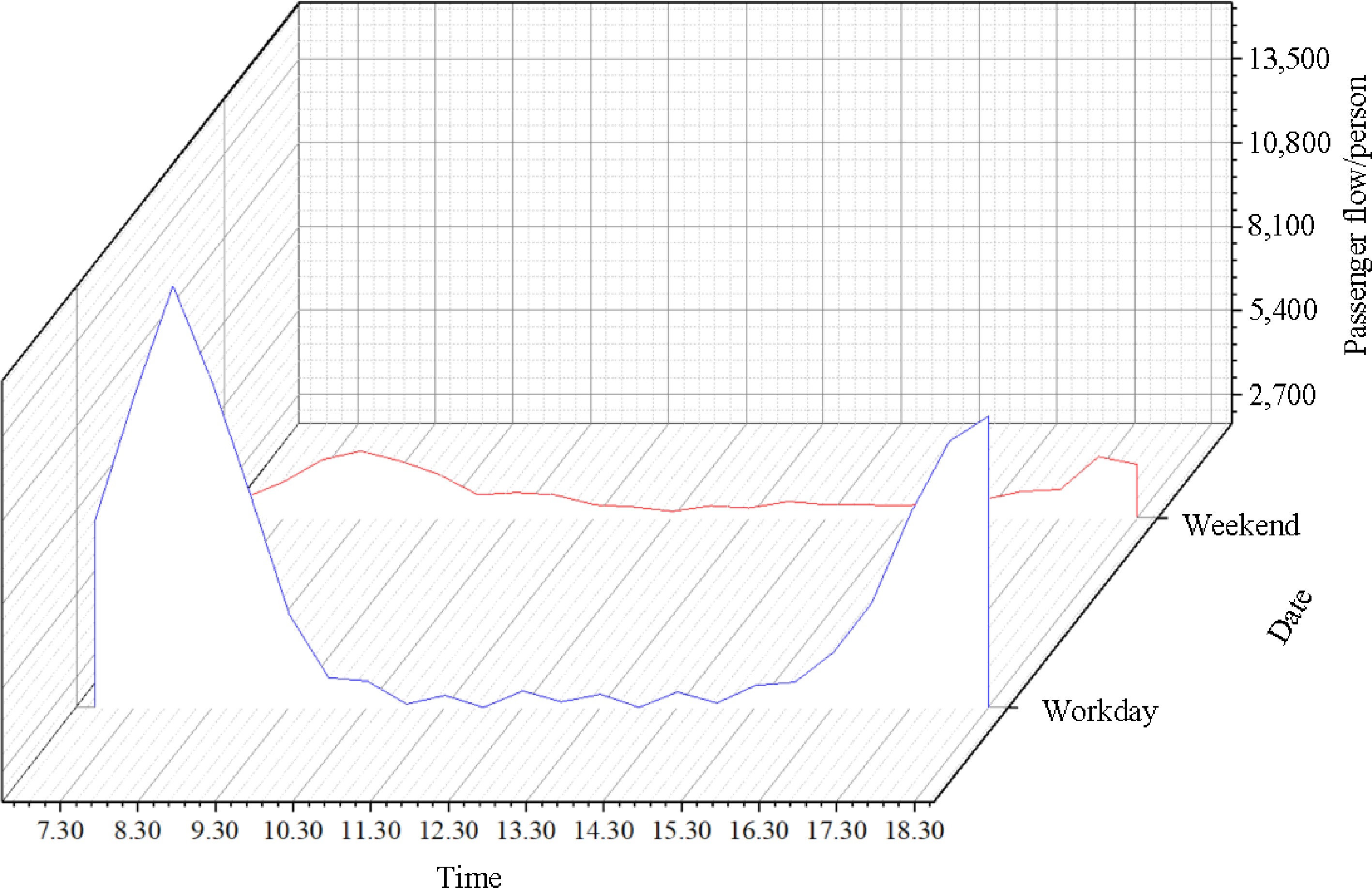
Figure 1. 

Distribution characteristics of hourly passenger flow at different periods.

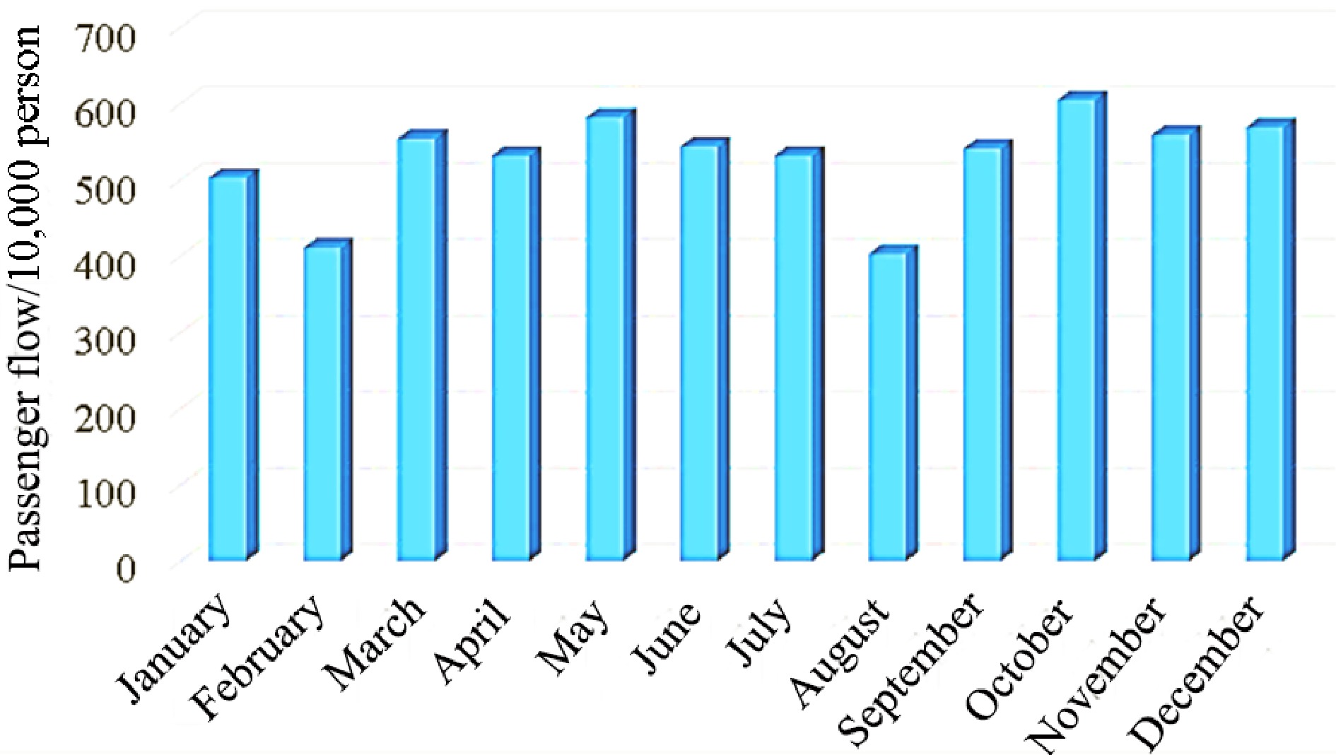
Figure 2. 

Monthly passenger flow distribution characteristics of rail transit.

Influencing factor data

Previous studies have shown that objective factors such as time segments (per hour), types of workdays, and weather have a significant impact on rail transit passenger flow. Therefore, data on these influencing factors during the study period is also essential. The data of weather, sourced from the National Meteorological Information Center - China Meteorological Data Network, is collected every 10 min and includes fields such as station number, date, 1-h precipitation, relative temperature, and humidity, and 10-min wind speed. Specific data fields and examples are shown in Table 2.

Based on the data collection and analysis, urban rail AFC card data can effectively reflect historical passenger flow characteristics under different spatial and temporal scenarios. Furthermore, the condition of influencing factor data provides a solid data foundation for our data-driven study of short-term urban rail transit passenger flow prediction.

Support Vector Regression (SVR) is an important extension of the Support Vector Machine (SVM) algorithm. Different from the SVM algorithm, which seeks to find the maximum-margin hyperplane to separate training samples of different categories, the SVR model aims to find a regression plane that minimizes the distance of all sample data from the plane. This approach incorporates slack variables to reduce the fluctuation range of passenger flow prediction results. The mathematical expression is as follows:

where, w represents the normal vector determining the direction of the hyperplane; b is the offset of the hyperplane from the origin; l is the total number of samples; x_i denotes the urban rail passenger flow input data; y_i signifies the passenger flow division output data. The core idea of the SVR model is to find a regression plane that makes all sample data close to it and to introduce a relaxation variable ξ to reduce the fluctuation range of the predicted urban rail passenger flow results. The mathematical expression is as follows:

where, the penalty factor C reflects the degree of penalty for sample data in the short-term passenger flow prediction model. The kernel function, |y − f(x)| > ε, is employed in the formula. By introducing the Lagrange function, the equation is transformed into its dual form, allowing for the solution of nonlinear regression problems. The SVR fitting function is mapped from low-dimensional to high-dimensional space as follows:

where, $ {\alpha _i} $ and $ \alpha' _{i} $ are Lagrange multipliers. Additionally, the model integrates the Gaussian Radial Basis Function (RBF) kernel, which is known for its good universality and noise resistance, changing the inner product space $ ({x}_{i}^{*},{x}_{j} $) into linear space. The expression for the short-term prediction SVR model of urban rail passenger flow using the Gaussian RBF kernel is as follows:

where, K(x_i,x) represents the power exponent of the Gaussian RBF kernel, and g denotes the bandwidth of the Gaussian kernel, where g > 0.

Improved Particle Swarm Optimization (IPSO) algorithm

Recent studies have indicated that the penalty coefficient $ C $ and the bandwidth parameter $ \text{g} $ of the kernel function in the Support Vector Regression (SVR) model significantly impact the accuracy and generalizability of the model's prediction results^[20]. While many studies used the manual parameter selection method or enumeration method to select parameter combinations, it is easy to miss the optimal parameter combinations and lead to low efficiency. Due to the inefficiency and low reliability of manual methods, it is considered more effective to use an intelligent optimization algorithm to optimize key parameters of the SVR model. The Particle Swarm Optimization (PSO) algorithm is fast, simple, and suitable for various optimization problems, it is sensitive to the initialization of the population. The rapid disappearance of its' particle diversity could lead to premature convergence, and the population has a single character, which makes the algorithm easy to fall into the local optimal solution. Besides, the PSO algorithm may converge to the local optimal solution when there is a large discrepancy in the initial population distribution. Therefore, this study proposed an improved the PSO algorithm to form an optimization algorithm for SVR model parameters.

Initially, the principle of the PSO algorithm is introduced. Derived from the study of bird flocking behaviour, each potential solution in the problem is considered a 'particle', and the particle's position represents the parameters (C,g). Each particle flies through the feasible solution space of the problem, updating its velocity and position based on its individual best position and the global best position. The fitness value of the objective function is used to evaluate whether the updated position of a particle is optimal. Through multiple iterations, the swarm of particles gradually approaches the problem's optimal solution. The principles for updating the particle's velocity and position are as follows:

where, $ {V}_{id}^{k} $, $ {V}_{id}^{k+1} $ are the moving velocities of particle i after the k^th and (k+1)^th iteration, i = 1, 2, ..., n. $ {X}_{id}^{k} $, $ {X}_{id}^{k+1} $ are the spatial positions of particle i after different iterations, representing a feasible solution of (C,g). $ {P}_{id}^{k} $ , $ {P}_{gd}^{k} $ are the optimal positions of particle i with respect to the whole particle population after the k^th iteration. c₁ and c₂ are the acceleration factors, representing the PSO's local and global seeking ability, typically set to 2. r₁, r₂ are random numbers, r₁, r₂ $ \in $ [0,1]. ω is the inertia weight, ω $ \in $ [0,1.4].

By comparing the fitness values of all particles, the optimal position update rule strategy for the entire particle swarm is obtained:

where, g(X) is the fitness function.

To further enhance the search efficiency and computational accuracy of the PSO algorithm, an Improved Particle Swarm Optimization algorithm (IPSO) is proposed, which incorporates a population selection strategy. The strategy involves dividing a population of N particles into dominant and inferior groups based on fitness values. The dominant group undergoes genetic crossover, while the inferior group undergoes mutation. Thus, we sorted and screened the fitness of particle swarm, selected the top 40% of particles to be iteratively updated directly, and the last 60% of particles were mutated first and then iteratively calculated. The expressions for these operations are as follows:

where $ {\underline{x}'_{i} }$ represents the generation of a new superior population; x denotes the particles in the dominant group sorted by fitness values. λ is the ratio for dividing the population into dominant and inferior groups ranges between 0 and 1. index1 and index2 are arrays arranged randomly with values ranging from [1, N'], where N', the number of particles in the superior solution group, equals half of the total population size, N/2.

The inferior group generates superior genes through mutation operations, thoroughly exploiting the information of each particle. The mutation calculation is as the following formula:

where $ \underline x'' _{i} $signifies the new population generated from the inferior group; $ {\underline x _i} $ is the i^th particle in the inferior group sorted by fitness values; f(t) = r₃(1 − t/G_max)², x_min and x_max represent the lower and upper bounds of the particle values; r and r₃ are random numbers between 0 and 1; t is the number of iterations; and G_max is the maximum number of iterations.

Subsequently, the processed population and the initial population at each iteration step are sorted by fitness values, and the top 30% of the particles are selected for the iterative update. As the number of iterations increases, the population size entering crossover and mutation operations gradually decreases, significantly accelerating the convergence speed in the later stages of iteration and enhancing the efficiency of the algorithm's solution.

The proposed IPSO algorithm is used to optimize key parameters in the SVR model. To quickly search the optimal values of SVR parameters [X_Cmin, X_Cmax] and [X_gmin, X_gmax] based on the PSO optimization algorithm, the search space position thresholds are set within specific limits. Thus, the urban rail passenger flow prediction model based on IPSO-SVR can be constructed. The calculation flow chart of the urban rail passenger flow prediction model based on the proposed IPSO-SVR algorithm is shown in Fig. 3.

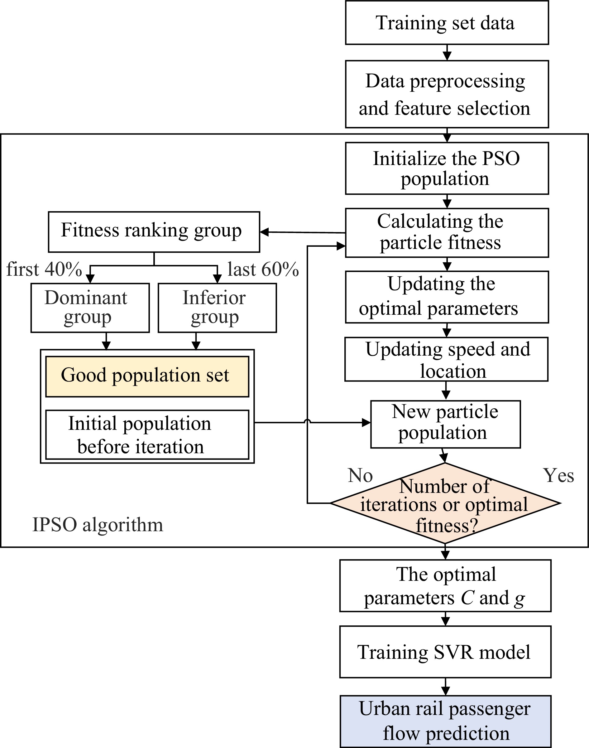
Figure 3. 

IPSO-SVR algorithm iterative calculation flow chart.

Model evaluation metrics

To measure the performance of the proposed passenger flow prediction model, mean squared error and relative accuracy metrics are used for comprehensive evaluation. Assuming the actual passenger flow value is y_i and the predicted value is $ {y'_{i}} $, with a sample size of n, the formulas for the evaluation metrics are as follows:

where, r represents the range threshold of absolute percentage error, which is set to 10%.

This study takes the Beijing Metro Line 4 as a typical urban rail line, selecting the 'Caishikou' station, which experiences high passenger traffic, as the subject of analysis. The research used rail AFC transaction data and influencing factor data from September 11^th to September 21^st, 2019, from 07:00 to 19:00, dividing the data into 30-min intervals for passenger flow analysis. The data was split into a training set and a test set at a ratio of 10:1.

Based on literature analysis and prior experience, PSO model parameters were set as follows: maxgen = 200, sizepop = 25, c₁ = 1.3, c₂ = 1.5, ω = 1, r₁ = r₂ = 1, eps = 0.0001, X_Cmin = 0.1, X_Cmax =100, X_gmin = 0.01, X_gmax = 1,000, θ = 0.6. The IPSO-SVR initial prediction model was optimized using passenger flow training set data and corresponding influencing factors. The fitness variation curve of the 'Caishikou' passenger flow is shown in Fig. 4. The results show that the optimal penalty coefficient C = 4.58 and kernel function parameter g = 0.87 for the urban rail passenger flow prediction model, with a global fitness value (MSE) of 0.0122.

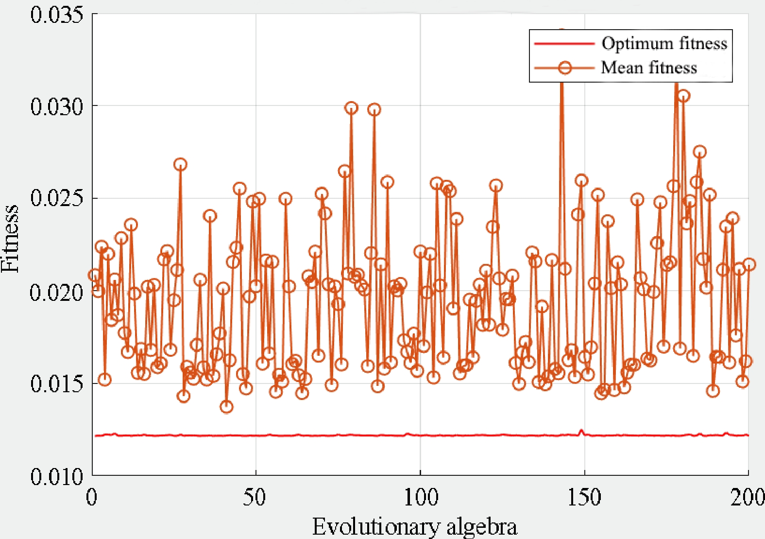
Figure 4. 

Change curve of model parameter population fitness value.

Results analysis

The IPSO-SVR passenger flow prediction model, trained with test set data and three influencing factors, was used to predict passenger flow for the 'Caishikou' rail station. The prediction results are reflected in Fig. 5.

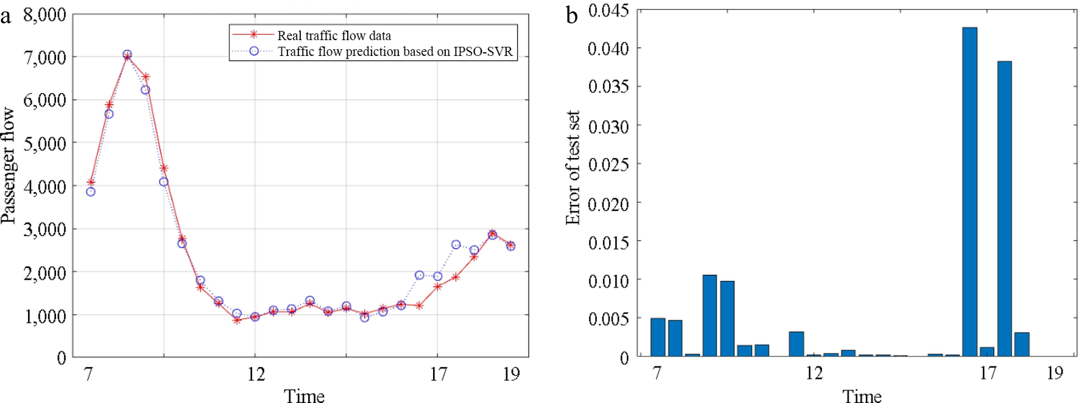
Figure 5. 

Results of IPSO-SVR passenger flow prediction model. (a) Passenger flow prediction results. (b) Mean square error.

It can be seen from Fig. 5 that the model prediction results are largely consistent with the actual data, exhibiting low volatility and deviation, effectively predicting the distribution characteristics and patterns of urban rail transit passenger flow. The prediction errors are generally low, suggesting that considering multiple influencing factors leads to predictions closer to real passenger flow data. However, there is a significant positive correlation between the model prediction errors and the scale of urban rail transit passenger flow. The higher prediction errors of urban rail passenger flow usually are produced in periods with higher passenger traffic intensity, such as during urban rush hours. Besides, the acceptable prediction results also show that the selected three influencing factors are effective.

To evaluate the effectiveness of the proposed IPSO optimization algorithm for the SVR model, the parameters of the SVR prediction model are optimized by the IPSO algorithm and the traditional grid method based on the passenger flow data from the training set of the 'Caishikou' station. The parameter search process of the SVR prediction model with the grid method is shown in Fig. 6. The optimal penalty coefficient C of the prediction model is 512, kernel function parameter g = 0.0625. Wherein, the initial values of the key parameters C and g are [2⁻¹⁰, 2⁻⁹, ..., 2¹⁰].

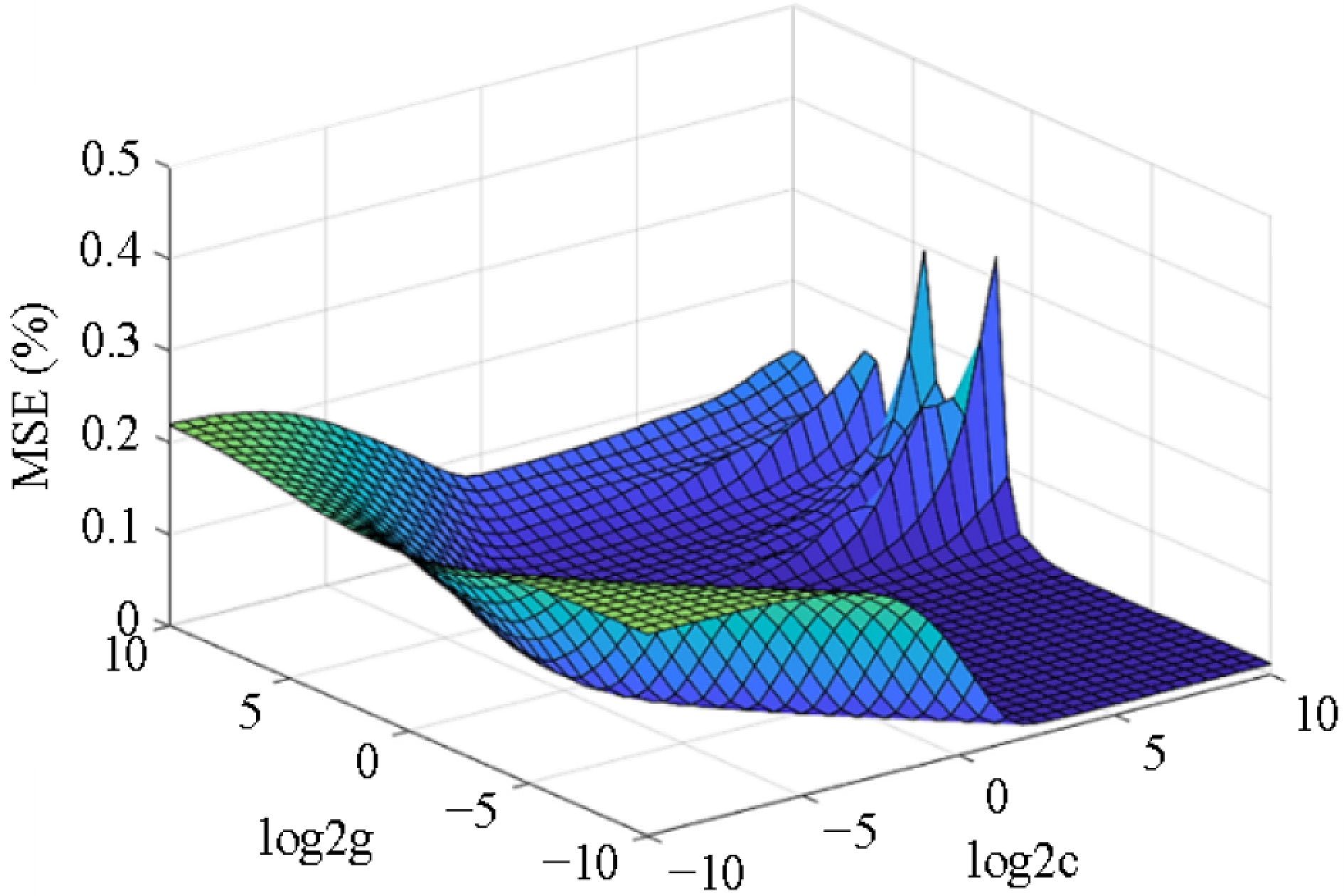
Figure 6. 

MSE curve of the SVR prediction model with the grid method.

According to the results in Fig. 4, the population best-fit value (MSE) of the IPSO algorithm for the optimal SVR model parameters is [0.013, 0.034]. The MSE of the SVR prediction model with grid method for the urban rail passenger flow in Fig. 6 is [0, 0.32]. Therefore, the fluctuation range of the grid method is significantly larger than that of the PSO algorithm, indicating that the parameters selection of the SVR prediction model optimized by the IPSO algorithm are more stable and applicable.

Further, to compare the performance of the proposed passenger flow prediction model, SVR and long short-term memory networks (LSTM) models were selected as comparative models. After training and predicting with relevant data, the passenger flow prediction values and model evaluation metrics of different models are shown in Fig. 7 and Table 3.

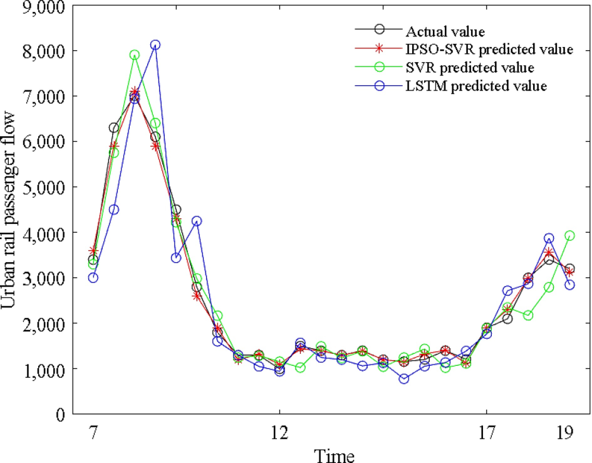
Figure 7. 

Results of passenger flow prediction based on different models.

The results, based on the model evaluation metrics in Table 3, indicate that the performance of the SVR model is inferior to the LSTM model, and the proposed IPSO-SVR model. This could be though the SVR model can mine the nonlinear influence of multidimensional features on passenger flow partially, but it is difficult to precisely capture the sequential correlations of multiple input variable features^[12]. Although the LSTM model can learn the sequential influence of multiple features on rail passenger flow, its accuracy in multi-factor coupled passenger flow prediction still needs improvement. The proposed IPSO-SVR model, by efficiently finding global optimal parameters and fully capturing multi-input variable data characteristics, shows higher mean squared error (1.54%) and relative accuracy (92.37%) than the other two comparative models.

In addition, to verify the predicting performance of the proposed IPSO-SVR model further, latsicNet, Bayesian Ridge, and linear regression in the previous study^[21] with a similar traffic environment are selected for the model performance comparison. Weng et al.^[21] used the XGBoost model to predict the urban road traffic performance index (TPI) of Beijing for four weeks from August 26^th to September 29^th, 2019. Traffic restrictions were implemented during the forecasting period, 4 d of rain, and the Mid-Autumn Festival holiday, which can reflect the prediction performance of the model under different factors. The MAE, MSE, and R² are selected as the model evaluation indicators of the prediction models. Though we use different models to predict different traffic indicies, the traffic index in the study by Wang et al.^[21] makes it easier to obtain higher prediction accuracy due to the smaller index value. We also used the traffic data in September 2019, Beijing (China), the same period and city indicates the background conditions of data of these two studies are consistent. Besides, the MSE is also adopted as our model evaluation indicator, which provides an optional index for comparative analysis of our research results.

The accuracy of the above three models is verified by the evaluation indicators, MSE of the compared models are 3.11%, 4.12%, and 3.56%, respectively, while the proposed IPSO-SVR model has the lowest value of MSE 1.54%. Model comparison results further confirmed and indicated the advantages of the proposed IPSO-SVR model in modelling the complex relationship between rail passenger flow and different influencing factors of rail network operation quality.

The study collected and analyzed the urban rail passenger flow AFC card data and related influencing factor data, then optimized the key parameters of the SVR prediction model using an improved Particle Swarm Optimization algorithm and proposed an IPSO-SVR-based urban rail passenger flow prediction method. The superiority of the proposed method was validated against evaluation metrics and compared with SVR and LSTM models. The research is conducive to further optimizing the line operation, vehicle scheduling, and passenger guidance of the traffic management enterprises.

The results show that the IPSO algorithm effectively optimizes the key parameters of the SVR model. The proposed IPSO-SVR model demonstrates higher accuracy in urban rail passenger flow prediction than conventional SVR and LSTM models, with a relative accuracy of 92.37%. Historical passenger flow data, combined with objective factors such as time segment information, types of workdays, and weather, can jointly depict the multi-dimensional factors and coupled characteristics of urban rail passenger flow, thereby improving prediction accuracy. The results reflect that the selected influencing variables and constructed short-time passenger flow prediction model are effective for predicting urban rail passenger flow.

However, this study also has some limitations, we just focused solely on algorithm design for accuracy evaluation and did not consider the impact of data scale and input variables on passenger flow prediction results. Also, we did not quantitatively analyze the reduction of the computation efficiency of the model after improving the PSO optimization algorithm, and the importance of different influencing factors to the model prediction results. Future research will further expand these aspects. Overall, this study provides support for the planning, operational organization, and dispatch optimization of urban rail transit.