Enhanced retrieval of forest parameters for vegetated areas in Guangxi province of China through synergistic integration of GEDI and Landsat 8

Forests are essential components of terrestrial ecosystems and play a crucial role in the global carbon cycle. Consequently, accurate assessment of forest resources is fundamental for a wide range of environmental studies, particularly those related to ecology and climate change^[1,2]. Mean forest canopy height (FCH), maximum FCH and aboveground biomass density (AGBD) are among the key variables used to describe forest growth and structure. These parameters are widely incorporated into ecological and climate-related models, and their accurate estimation can effectively reduce uncertainties in related studies^[3].

It is time-consuming and inefficient to conduct forest ground surveys in large areas. Remote sensing technology provides a timely, accurate, and efficient method for forest resource monitoring^[3−5]. Over the past two decades, LiDAR has substantially advanced forest resource monitoring by enabling direct observation of three-dimensional forest structure. In contrast, traditional optical and microwave remote sensing mainly provide surface information of ground objects^[6−8].

Airborne Laser Scanning (ALS) and Unmanned Aerial Vehicle (UAV) systems are often cost-prohibitive and impractical for large-scale applications. Satellite-based forest parameter data has primarily relied on instruments like NASA's GLAS (ICESat) and ATLAS (ICESat-2) LiDAR. While these instruments have been valuable, they are not specifically optimized for vegetation mapping^[9−11]. The introduction of the NASA Global Ecosystem Dynamics Investigation (GEDI) has been a significant development in this field. GEDI, a spaceborne LiDAR instrument mounted on the International Space Station (ISS), has been operational since April 2019. It provides global coverage (51.6° N–51.6° S) for vegetation structure measurements, offering a wealth of data for various scientific objectives, including biomass estimation and carbon budget modeling^[6]. The footprint-level products provided by GEDI cannot be directly applied to regional studies^[11]. Establishing regression relationships between LiDAR and optical or microwave information involves the integration of various modeling approaches, including data-driven models or physical models^[12]. Approaches can be classified as either parameter-reliant or parameter-independent.

Parametric methods typically include statistical regression methods. A multiple regression model was used to integrate GLAS LiDAR, spectral information, field survey data, and land classification data to create a AGB map (R² = 0.43–0.67) in China^[13]. MODIS data was utilized to extrapolate GLAS-derived vegetation heights (R² = 0.67)^[9]. Non-parametric approaches, such as Random Forest (RF), have become common methods for obtaining spatially-exhaustive estimates due to the inability of parametric approaches to meet the assumptions and prior knowledge of certain parameters. These approaches are suitable for datasets where predictors include both categorical and continuous variables^[10,14,15]. GEDI products based on Landsat spectral information were extrapolated to generate a global FCH map (RMSE = 9.07 m; R² = 0.61)^[16].

Despite these advancements, several key challenges remain for large-scale forest parameter estimation: (1) Signal Saturation and Feature Extraction: in dense, high-coverage forests, both LiDAR penetration capability and optical spectral signals face saturation, making accurate feature extraction difficult, especially for complex vertical and horizontal structures. (2) Model Suitability and Optimization: non-parametric methods like Random Forest (RF) are common but require careful assessment of model suitability, considering computational speed, parameter complexity, and accuracy^[17,18]. Every machine learning model involves hyperparameters that demand extensive expert tuning. (3) Scalability and Generalization: extrapolating relationships from sparse LiDAR footprints (e.g., GEDI) to continuous maps over complex and varied terrain introduces significant uncertainty, and current methods often struggle to balance accuracy with computational efficiency for regional applications.

Recently, automated machine learning (AutoML) has emerged as a promising strategy for improving model development efficiency. By integrating algorithm selection, hyperparameter optimization, and model evaluation into a unified workflow, AutoML can identify competitive solutions under limited time and computational budgets^[19]. This is particularly valuable in remote sensing applications, where model performance often depends strongly on manual hyperparameter tuning and model selection. This approach ensures fairness in model comparisons while enhancing research efficiency and reproducibility^[20]. Conversely, the existing applications of AutoML in remote sensing has often relied on limited feature sets without systematically integrating multi-scale or multi-sensor inputs, while also inadequately addressing spatial heterogeneity and scale effects in complex forest environments. Moreover, there has been limited exploration of advanced feature types—such as Fourier-based texture descriptors—within fully automated modeling workflows.

In this study, we propose an AutoML-based framework for large-scale retrieval of forest structural parameters in dense and topographically complex regions. The framework integrates spaceborne LiDAR observations with multi-source remote sensing predictors, including FOTO-derived texture features. We further evaluate its performance in Guangxi, China, across mean FCH, maximum FCH, and AGBD.

This study established relationships between GEDI-derived response variables and satellite-based predictor variables using an AutoML framework, and then produced large-area maps of mean FCH, maximum FCH, and AGBD. The workflow is illustrated in Fig. 1. First, high-quality GEDI footprints were screened. Highly correlated variables were removed, mainly among spectral features, vegetation indices, and GLCM texture metrics. Mean and maximum FCH were calibrated using selected RH metrics from GEDI L2A, while AGBD was obtained from GEDI L4A. We then constructed a multi-dimensional predictor set for each GEDI footprint, including spectral features, vegetation indices, GLCM texture metrics, FOTO-derived texture features, and ancillary topographic data. Finally, the trained models were applied to the full study area, and the resulting maps were further evaluated in terms of model performance, feature importance, and spatial distribution patterns.

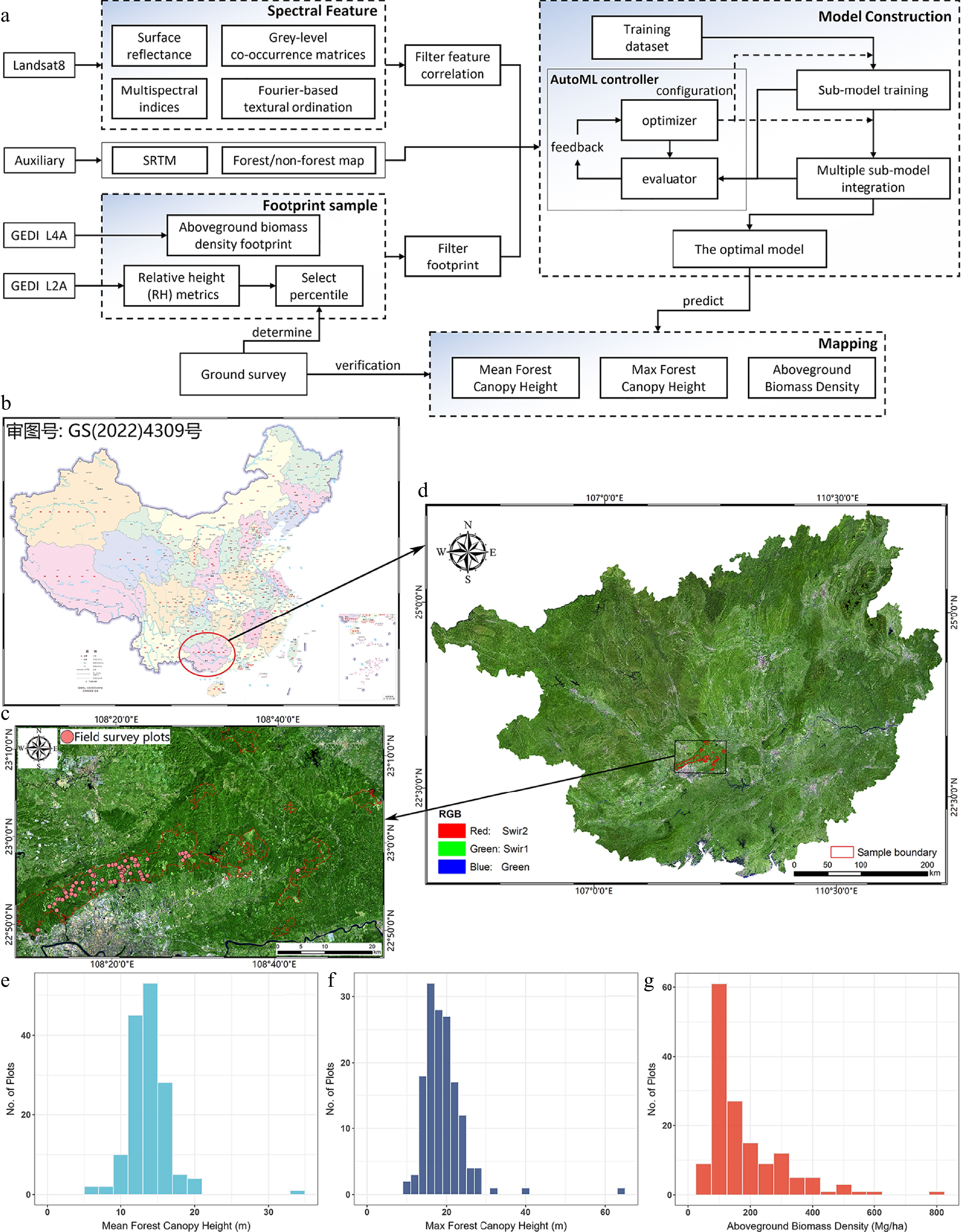
Figure 1. 

(a) Flowchart of proposed methods. The study area is located in Guangxi Province in China. The ground survey area is located in (b) Gaofeng forestry, with (c) red boundary and pink field survey plots. (d) The overview of the study area. The distribution of (e) mean FCH, (f) max FCH, and (g) AGBD.

Study area

Guangxi Zhuang Autonomous Region (shown in Fig. 1d, referred as Guangxi) is located in southern China (104°26'–112°04' E, 20°54'–26°24' N) and is characterized by complex terrain, high forest cover (over 60%), and diverse vegetation types. The terrain of Guangxi is sloping from northwest to southeast, with low terrain in the southeast and high terrain in the northwest. The land area of the province is about 236,700 km² with an average altitude of 1,000–1,500 m, an average annual rainfall of 1,835 mm, and an average annual temperature of 21.1 °C. Major vegetation types include monsoon rain forest, evergreen broad-leaved forest, coniferous forest, deciduous broad-leaved forest, mixed evergreen deciduous broad-leaved forest, bamboo forest, scrub, etc. In addition, there are large areas of plantation forests, mainly of horsetail pine, eucalyptus (Eucalyptu ssp), fir, and moso bamboo (Phyllostachys pubescens). The region spans tropical to subtropical climatic zones from south to north, providing a representative setting for large-scale forest parameter estimation.

The field survey area is located at the Gaofeng State Forest Farm (referred to as Gaofeng forestry), with over 40,000 hm² of forest area and approximately 87% forest coverage. The sample boundary of Fig. 1c shows the extent of the forest survey area. The surveyed stands are dominated by plantation forests, including China fir (Cunninghamia lanceolate), Masson pine (Pinus massoniana), and Slash pine (Pinus elliottii). Broad-leaved forests are mainly Eucalypt hybrid urograndis (Eucalyptus grandis × urophylla), Ampupu (Eucalyptus urophylla), Spingbract Chinkapin (Castanopsis hystrix), Oil tea (Camellia oleifera), and so on^[21]. To provide a basis for model development and testing, 150 field survey plots, each 20 m × 30 m, were investigated from October to November, 2022. Based on a survey of 1,797 trees, the study area predominantly features Cunninghamia lanceolata, Eucalyptus grandis × urophylla, and Eucalyptus urophylla, mostly in pure stands. The approximate distribution (Fig. 1e−g) is within 6 to 34 m, 10 to 64 m, and 57 to 788 Mg/ha, respectively. The median plot values are 14 m, 18 m, and 132 Mg/ha, respectively.

Earth observation data

The GEDI data collected between January 1 and December 31, 2022, provide waveform return metrics (from https://search.earthdata.nasa.gov/). The GEDI Level 2A (L2A) Version 2 Elevation and Height Metrics products are available from the NASA/USGS Land Processes Distributed Active Archive Center^[22]. Each footprint provided a series of relative height (RH) metrics, indicating percentiles of energy return height relative to the ground. The GEDI Level 4A (L4A) Version 2 provides predictions of AGBD and estimates of prediction standard error within each geolocated laser footprint. Data for each of the eight beams includes uncertainty metrics, quality flags, model inputs, and other information related to the GEDI Level 2A waveform for the selected algorithm setting group^[22].

Landsat 8 OLI/TIRS Collection 2 surface reflectance data were used as the primary optical predictor dataset. This dataset contains atmospherically corrected surface reflectance and land surface temperature derived from the data produced by the Landsat 8 OLI/TIRS sensors. Cloud masking and image preprocessing were conducted on the Google Earth Engine (GEE) platform (https://earthengine.google.com) using images acquired between March 3 and October 31, 2022.

Additional ancillary datasets included SRTM-derived elevation, slope, and aspect, as well as a forest/non-forest map. Elevation data was obtained from the NASA SRTM product (https://search.earthdata.nasa.gov/), while slope and aspect were derived from the DEM within GEE. The forest/non-forest product was obtained from the CASEarth dataset (https://data.casearth.cn).

AutoML and model selection

AutoML frameworks utilize ensemble methods such as stacking, and weighted combinations^[23]. In shallow stack ensembling (Table 1), individual base models are trained separately in parallel on the same instance, and their aggregated predictions serve as features for a stack ensembling model. To optimize performance, AutoML employs K-fold ensemble bagging across all model layers, dividing data into K disjoint chunks for training and validation. Each model iteration produces out-of-fold predictions, which are averaged over N random partitions to fit time constraints. Multi-layer stacking integrates stacker model predictions as inputs for higher-level stackers, culminating in an ensemble selection to aggregate predictions^[24].

We utilized the H2O platform, an open-source, distributed, and scalable machine learning and predictive analytics platform. H2O enables machine learning model development on large datasets, featuring widely used algorithms, model interpretation capabilities for regression, and interactive user interfaces. H2O's AutoML was selected for its scalability, ensemble stacking capability, and efficient runtime performance compared to alternatives like Auto-Sklearn and TPOT, which aligned with the study's need for both predictive accuracy and explanatory insight. Six typical machine learning models were selected for experimentation: (1) Deep Learning (DeepL); (2) Distributed Random Forest (DRF); (3) Gradient Boosting Machine (GBM); (4) Generalized Linear Models (GLM); (5) Stacked Ensembles (SE); (6) Extremely randomized trees (XRT). Our AutoML setup involved 5-layer stacking (T = 5) with repeated 5-fold bagging (K = 5), and 3 repeats (N = 3) to make full use of the available computational budget. We controlled model training saturation by setting the maximum number of models to 20, using root mean square error (RMSE) as the stopping metric (stopping_rounds = 3 and stopping_tolerance = 0.01).

Fourier-based textural ordination

Fourier-based textural ordination (FOTO) quantifies texture variation gradients by analyzing the two-dimensional Fourier spectra of canopy scene images^[25,26]. The method consists of the following key steps: first, a window size is defined and the image is divided into unit windows, each represented by a matrix of pixel spectral radiance values. Subsequently, two-dimensional Fast Fourier Transform (FFT) is applied to decompose the spatial information of the image, capturing variations in canopy structure across different spatial frequencies. The squared amplitudes are computed to generate a two-dimensional periodogram, which allocates radiance variance across frequency bins. Next, the FFT amplitudes are squared and averaged to produce a radial spectrum (r-spectrum), extracting scale information, where each radial spectrum reflects the wavenumber frequency distribution, characterizing the repetition of sine/cosine patterns in canopy texture. Finally, standardized Principal Component Analysis (PCA) is performed on the radial spectra, with the first three principal components (R, G, B) serving as texture indices to order windows along texture gradients and describe canopy texture features^[27].

In practical implementation, this study follows established methodologies and introduces optimizations. Given the superior performance of the near-infrared (NIR) band in biomass mapping^[26], a window size of 100 × 100 pixels was selected for FOTO feature extraction on NIR band images. The process included dividing the image into windows, generating periodograms, converting them to radial spectra, and extracting the first three principal components via PCA as foundational texture indices. To further mitigate windowing effects and enhance spatial continuity, a multi-scale strategy was adopted, repeating the same procedure with additional window sizes of 30 × 30, 50 × 50, and 80 × 80 pixels. The selected scale gradient aims to capture texture features of forest canopies in the study area, ranging from fine to coarse, thereby generating a comprehensive set of texture features that characterize canopy structures across multiple spatial scales.

Selection of samples and features

Selecting high-quality GEDI footprints effectively reduces uncertainty in model inputs. For filtering valid samples, both GEDI Level 2A and Level 4A data were subjected to the following common criteria. Only footprints acquired in full-power laser mode during nighttime were retained, requiring the best geolocation quality (degrade_flag = 0)^[16] and a beam sensitivity no less than 0.9^[28]; footprints located on slopes greater than 30° were also excluded to ensure the accuracy of terrain and canopy height retrieval^[29]. This threshold was applied as a conservative quality-control criterion for GEDI reference samples, because waveform signals over steep terrain are more susceptible to terrain-induced broadening and mixing, which may increase the uncertainty in ground-canopy separation and consequently affect the reliability of canopy height and biomass retrieval. Additionally, Level 4A data were further filtered using specific criteria. Only observations with a predicted AGBD of no less than 0 Mg/ha were selected, requiring sufficient waveform fidelity (algorithm_run_flag = 1), and unreliable measurements with a relative standard error of AGBD exceeding 50% were removed^[30]. The filtered data exhibited varying distributions, ranging from 3,100 to 42,000 samples per 50 km × 50 km Landsat tile. For fewer than 10,000 footprints available, this was supplemented with footprint samples of the same track from neighboring tiles. This filtering yielded a dataset of at least 2 million GEDI samples.

We constructed a set of predictor variables (Table 2) that included spectral features, vegetation indices, topographic variables, and texture metrics. Spectral predictors were derived from Landsat 8 bands 2–7, while topographic variables included elevation, slope, and aspect derived from the SRTM DEM. Texture-related predictors included both GLCM metrics and FOTO features. GLCM-based texture measures, associated with a 9 × 9 window size, and six Landsat 8 bands were applied in experiments.

In total, 86 predictor variables were generated. After correlation analysis, the GEDI samples were randomly divided into training (70%) and validation (30%) sets. To establish local relationships between LiDAR-derived responses and predictor variables, the study area was partitioned into 50 km × 50 km tiles, each containing an average of approximately 23,000 footprints. The entire Guangxi region was divided into 145 tiles.

We first conducted experiments in the field survey area (Fig. 1c) before this approach was extended on a large scale (Fig. 1d). We systematically applied a suite of standard statistical metrics to quantify model performance. The primary evaluation was based on the Root Mean Square Error (RMSE), which provides a comprehensive measure of the average magnitude of prediction errors. To complement this, we calculated the Mean Absolute Error (MAE) to assess the typical absolute deviation between predicted and observed values, thereby offering a more intuitive measure of error magnitude. Lastly, we incorporated the Bias metric to quantify the average direction of prediction errors, specifically identifying systematic overestimation (positive bias) or underestimation (negative bias). The mean FCH, max FCH, and AGBD per quadrat were recorded in the sample plot. The average estimates of Landsat 8 pixel center coordinates falling within the sample plots were compared with the field survey values. We used a comparison of the field survey mean and max FCH, within the Landsat pixel, with GEDI waveform return metrics to select the best GEDI metric as training data for the Landsat-based mean FCH and max FCH model. We analyzed 13 GEDI relative height (RH) metrics, RH45–RH100 (Table 3). We found that the RH55 and RH95 metrics were in the best agreement with the field survey data. The modeling results for other metrics deviate further from the validation data. Therefore, the RH55 and RH95 metrics were selected as the training variables to calibrate the mean and max FCH models.

In addition to FCH, we tested the accuracy of the estimated AGBD. We summarize the validation results of forest parameters mapping in Gaofeng forestry in Table 4. The validation results indicate considerable uncertainty in forest parameter estimation, particularly for AGBD. Nevertheless, the predicted values remained broadly consistent with the field observations, suggesting that the models were able to capture the general magnitude and variation of the target variables. For mean FCH, the model yielded an RMSE of 5.63 m and a bias of −2.67 m. For maximum FCH, the RMSE and bias were 7.21 m and −2.99 m, respectively. AGBD showed larger uncertainty, with an RMSE of 81.0 Mg/ha and a bias of −36.50 Mg/ha. We extended the experimental approach in the Gaofeng forest to a larger area for further experimental analysis.

Modeling results of forest parameters

We established the relationship between LiDAR response and Earth observation features, and extended the experiment of forest parameter estimation to Guangxi province.

Spatial distribution of forest parameters

Spatially, anomalously high LiDAR-response footprints remain visible in the mapped products, particularly in areas with very high forest parameter values (Fig. 2a−c). The models tended to underestimate extremely high values, whereas low- to medium-value areas showed relatively smoother and more coherent spatial patterns. In intermediate-value regions, the inclusion of FOTO features helped enhance local structural discrimination, although this improvement was accompanied by reduced spatial smoothness in some areas. In high-value regions, spectral and structural saturation likely limited the ability of the models to preserve spatial continuity while maintaining footprint-level accuracy.

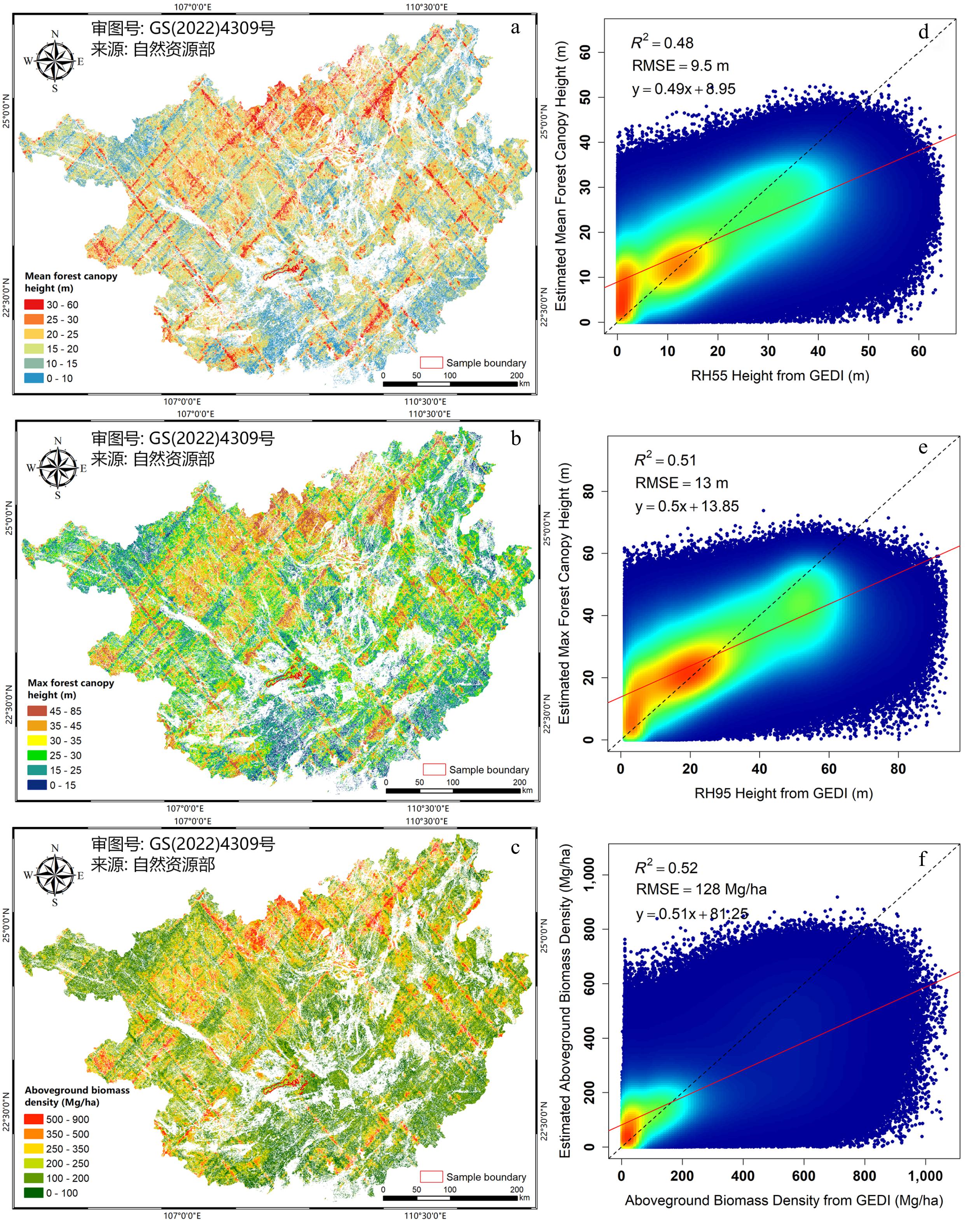
Figure 2. 

The mapping results of the (a) mean FCH, (b) max FCH, and (c) AGBD. (d)–(f) The scatter plots of the corresponding results of test sets, respectively.

Analysis of model performance

We performed a total of 145 model training rounds in Guangxi Province. The GEDI samples with features were randomly separated into training (70%) and validation (30%) datasets. The R² for mean FCH validation (Fig. 2d) was 0.48 (RMSE = 9.5 m). The mean FCH ranging from 5 to 30 m exhibited moderate errors (RMSE = 5.8 m), whereas heights between 0 and 5 m are significantly overestimated (RMSE = 7.0 m), and heights greater than 30 m are markedly underestimated (RMSE = 11.3 m). The R² for max FCH validation (Fig. 2e) was 0.51 (RMSE = 13.0 m). The max FCH ranging from 15 to 45 m exhibit moderate errors (RMSE = 7.6 m), whereas heights between 0 and 15 m are significantly overestimated (RMSE = 10.0 m), and heights greater than 45 m are markedly underestimated (RMSE = 14.4 m). The R² for AGBD validation (Fig. 2f) was 0.52 (RMSE = 128 Mg/ha). The AGBD ranging from 50 to 200 Mg/ha exhibit moderate errors (RMSE = 62.8 Mg/ha), whereas values between 0 and 50 Mg/ha are significantly overestimated (RMSE = 66.9 Mg/ha), and values greater than 200 Mg/ha are markedly underestimated (RMSE = 156.9 Mg/ha).

Figure 3 summarizes the RMSE distributions of the candidate models across all training runs. Model performance was jointly influenced by predictive accuracy, stability across runs, and the effective search space explored during AutoML optimization. For mean FCH (Fig. 3a), DRF, GBM, and SE (mean RMSE = 9.84, 9.73, and 9.26 m) showed the strongest overall performance, with SE achieving the lowest mean RMSE. The difference between the upper quartile and the lower quartile, measured by the interquartile range (IQR), reflects the stability of the model's performance across runs. The corresponding IQR values for DeepL, DRF, GBM, GLM, SE, and XRT are 1.15, 0.82, 1.12, 0.86, 0.79, and 0.99 m, respectively. The frequency percentage (Fig. 3a) of DeepL, DRF, GBM, GLM, and XRT models integrated into the SE model was 20%, 6%, 63%, 6%, and 6%, respectively. Similar patterns were observed for maximum FCH (Fig. 3b) and AGBD (Fig. 3c), where SE consistently outperformed the single-model approaches.

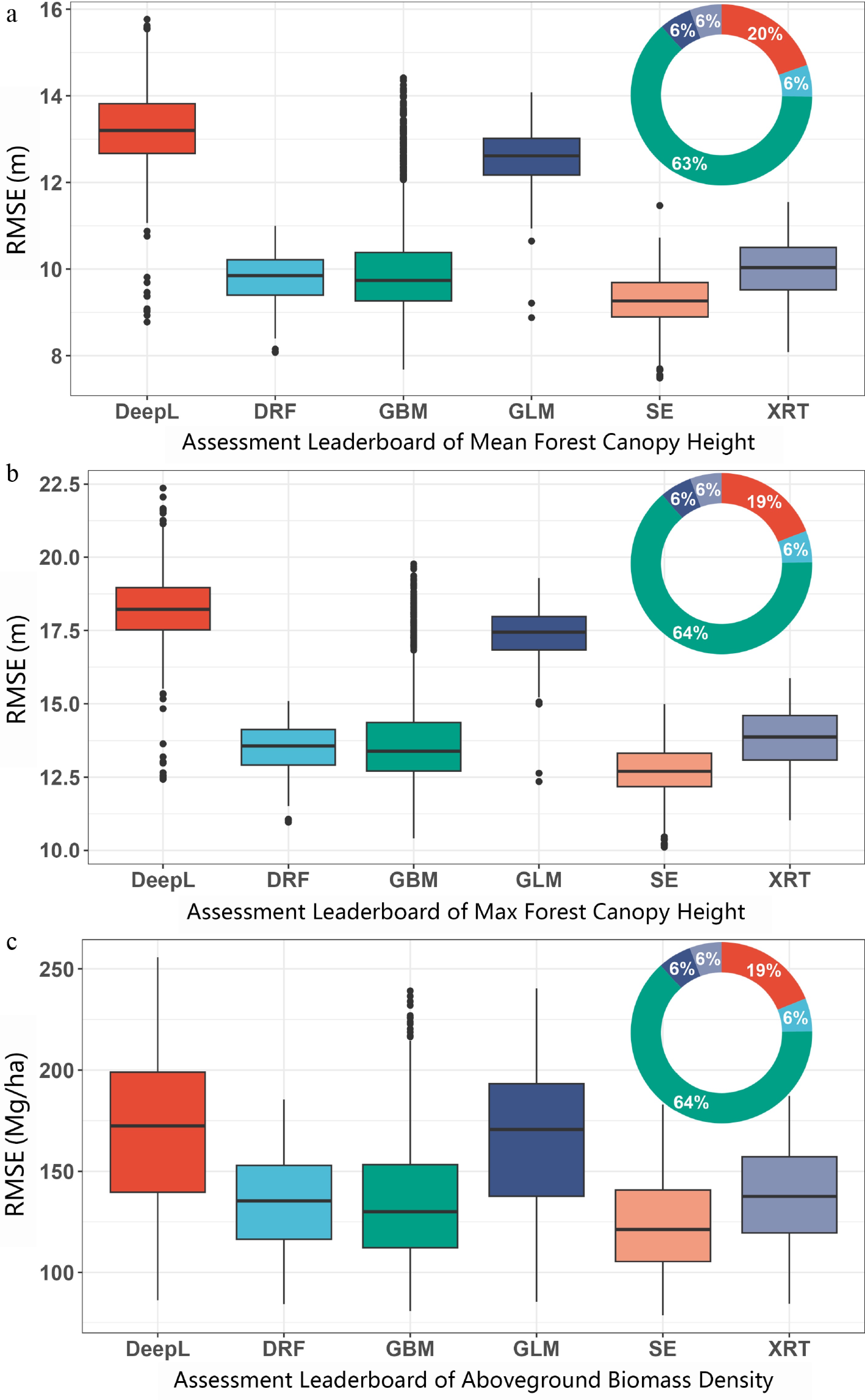
Figure 3. 

The RMSE of models trained by AutoML in (a) mean FCH, (b) max FCH, and (c) AGBD mapping. The frequency percentage in the pie chart is of the best performing SE model in sub-model combination from the model building process.

The SE models were constructed from multiple base learners, with GBM and Deep Learning contributing most frequently to the final ensembles. This indicates that AutoML consistently favored models that balanced strong predictive accuracy with sufficient model flexibility. The stable behavior of SE across the three target variables suggests that the ensemble strategy provided robust performance for large-area mapping.

We defined an initial set of 86 features. Many of these features are highly correlated, especially some spectral indices. Features that have high a correlation with multiple features were removed first. Through the Pearson correlation analysis in Guangxi area (approximately 400 million points), we removed all highly correlated features (correlation $ \geq $ 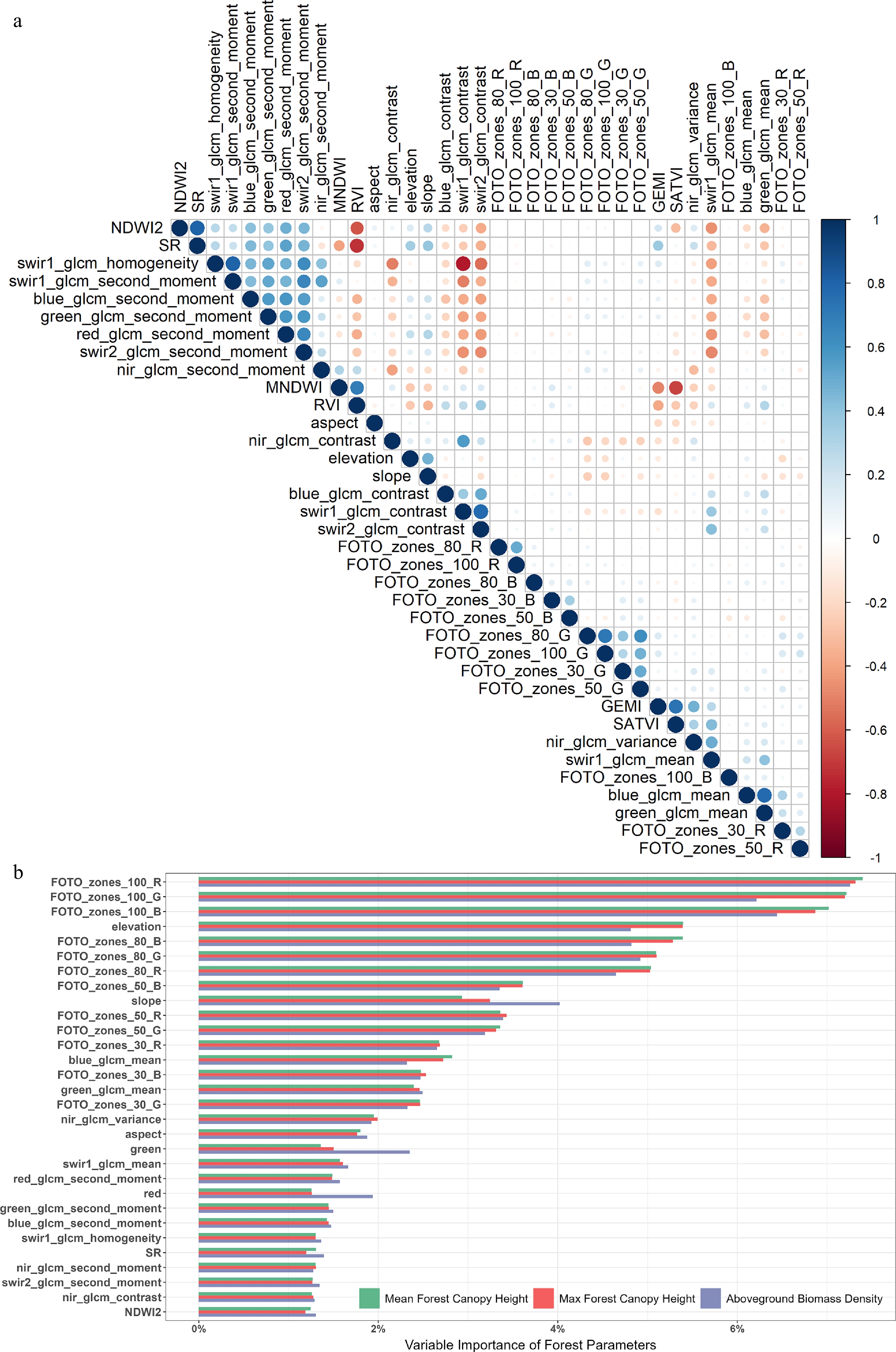0.8), leaving only 46 features to participate in subsequent experiments. Figure 4a shows only the filtered features to enhance the readability of the content. It is worth noting that both FOTO features of any size window have very little correlation with other features. As the window size increases, the correlation between FOTO and other features gradually tends to be uncorrelated.

Figure 4. 

(a) Linear relationship plot between each feature. Only the results of the filtered features are shown here. (b) The variable importance of regression models was calculated in mean FCH, max FCH, and AGBD mappings within the whole Guangxi province. Variables have been sorted according to their importance, and each variable was defined in Table 2. Only the top 30 features are shown here.

In the process of establishing regression relationships between forest parameters and features, the effects of some features are negligible. We remove these features through variable importance experiments, which can improve modeling efficiency while affecting only a small amount of modeling accuracy. Variable importance is calculated by the relative influence of each feature: whether that feature was selected during the model-building process, and how much the squared error improved (decreased). Then, the squared error was normalized to be between 0 and 1. Figure 4b presents the average variable importance of the top 30 features used in training models for three forest parameters (mean FCH, max FCH, and AGBD). The first 30 variables explain 88.6%, 88.7%, and 87.6% of the model components, respectively. The remaining 16 variables have only approximately 10% of the explanatory ability and could be discarded at the cost of an acceptable reduction in R² of 0.01 or less. It could be considered that the whole model could be roughly explained. The abandoned features are mainly spectral information, spectral indices, and the GLCM contrast features. We focus on the properties of the first 30 variables. For the three forest parameters, the feature importance does not differ largely, with only some minor variations. Modeling forest parameters is very difficult, and the top-ranked variable only explains less than 10% of the model components.

The top three variables are FOTO_zones_100 (R, G, B). These three variables could explain 21.6%, 21.4%, and 19.9% of the components of the models, respectively. The feature of nir combined with a window of 100 size plays the most critical role. If there is a panchromatic band added to the operation, maybe it is also an important variable^[26]. The top ten variables (mainly features, FOTO_zones_100, and FOTO_zones_80) provided 52.8%, 52.5%, and 49.9% of the explanation of the model components. As the number of variables increases, the explanatory ability of the variables decreases gradually. While the number of variables is up to 20 (mainly features, FOTO_zones_100, FOTO_zones_80, FOTO_zones_50, and surface elevation), the explanatory model ability reaches about 75.4%, 75.5%, and 73.4%, respectively. The FOTO features provide 55.1%, 54.8%, 51.7% of the explanatory ability, respectively. FOTO features contributed substantially to model performance, indicating that canopy texture provided structurally meaningful information beyond spectral variables alone^[53,54]. The three principal axes (R, G, B) can correlate the stand parameters and biomass dynamics of the different land-use types^[27]. Topographic variables also played an important role, likely because elevation-related gradients in temperature, moisture, and vegetation composition influence forest growth and structure. Finally, we selected only the top 30 features for the experiment. Although FOTO variables contributed strongly to the model, this does not mean that the regression relied on texture information without constraint. To reduce redundancy and overfitting risk, the original 86 variables were first reduced to 46 using Pearson correlation analysis, and only the top 30 variables were retained for the subsequent experiments. Moreover, FOTO features were incorporated together with spectral, topographic, and other texture-related predictors, rather than being used alone. In preliminary tests, larger FOTO scales could further improve apparent fitting accuracy, but also produce more obvious scale dependence and overfitting tendency. Therefore, the adopted multi-scale FOTO setting was chosen as a balance between explanatory ability and generalization performance. This suggests that the high importance of FOTO reflects its strong structural relevance to forest parameters, while the selected configuration helps maintain model robustness.

Comparative experiments of FOTO

The variable importance analysis indicated that FOTO was a major contributor to model performance. To further evaluate its effect, we compared the regression results before, and after including FOTO features in three representative sample areas (Fig. 2b). The results showed that incorporating FOTO substantially improved the estimation of mean FCH, maximum FCH, and AGBD, particularly in areas with relatively high parameter values (Fig. 5), where establishing stable regression relationships is more challenging. Across the three target variables, the inclusion of FOTO increased R² by 0.31, 0.29, and 0.32, respectively, while reducing RMSE by 2 m, 3 m, and 33 Mg/ha. By contrast, the models without FOTO showed only weak correlations (R² ≈ 0.1−0.3), indicating that texture information provided substantial additional structural information.

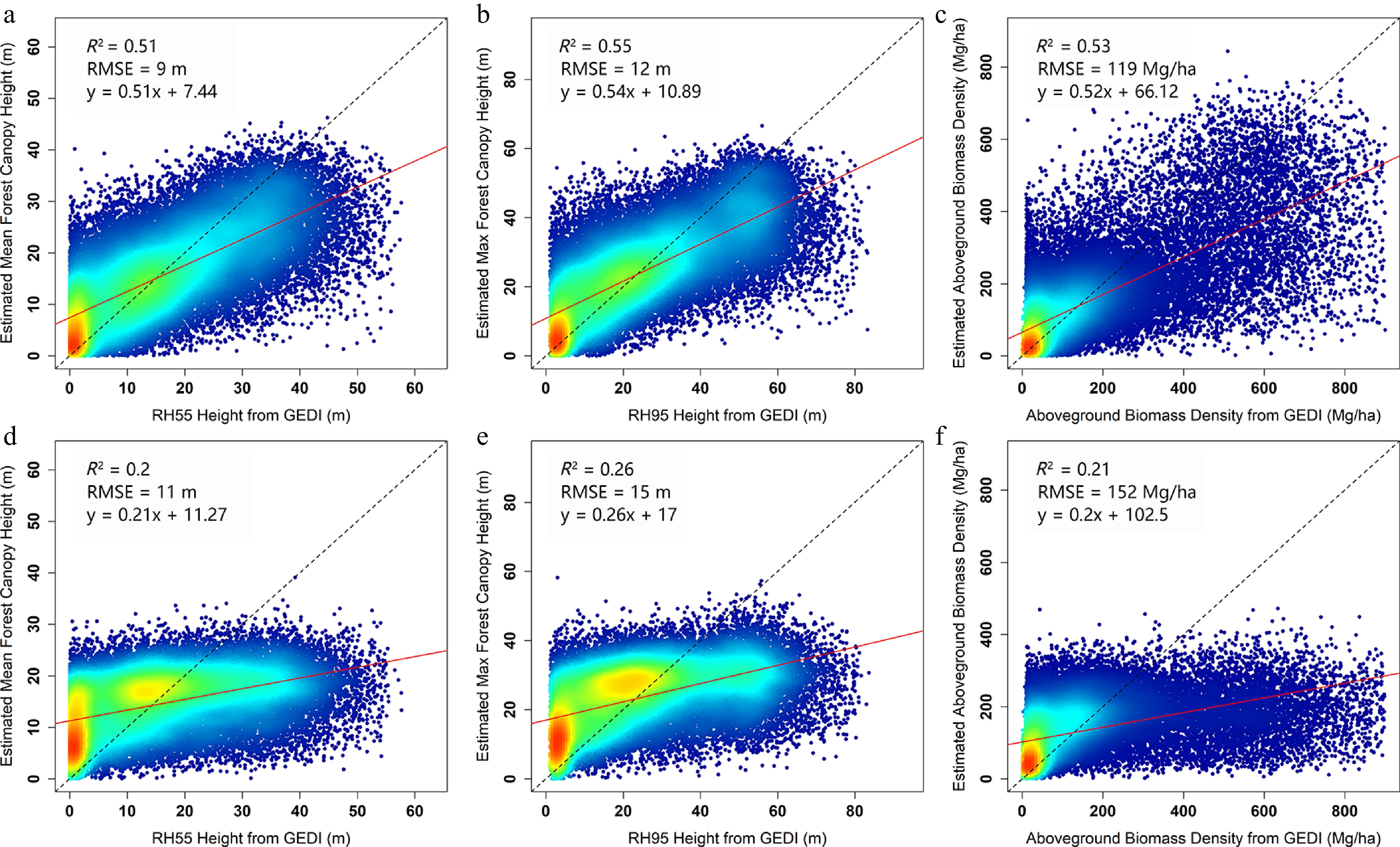
Figure 5. 

Scatter plots measuring the enhancement of FOTO features on the regression ability of model training. (a) and (d) show the scatter plots of mean FCH regression model training after adding FOTO features for sample areas respectively. (b) and (e) show the scatter plots of max FCH regression model training after adding FOTO features for sample areas respectively. (c) and (f) show the scatter plots of AGBD regression model training after adding FOTO features for sample areas.

At Landsat 30-m resolution, FOTO should not be interpreted as resolving individual tree crowns. Instead, each 30-m pixel contains a mixed canopy signal from multiple crowns, gaps, shadows, understory vegetation, and background components. Therefore, the FOTO features derived in this study represent the spatial-frequency organization of canopy reflectance among neighboring 30-m pixels, rather than single-tree geometry. Because the adopted window sizes correspond to spatial extents of approximately 0.9–3.0 km, the derived texture gradients are better interpreted as stand- to patch-scale descriptors of canopy continuity, gap distribution, and forest fragmentation. In this sense, FOTO captures whether neighboring forest pixels form smooth and continuous canopy neighborhoods or irregular and fragmented patterns. High-biomass forests usually exhibit more continuous canopy cover, lower gap fraction, and stronger structural organization at the stand and patch scales, whereas low-biomass or disturbed forests tend to show greater discontinuity, fragmentation, and local heterogeneity. As a result, FOTO provides structurally meaningful information beyond spectral indices alone, which is particularly valuable in dense forests where spectral responses are more prone to saturation. This scale-dependent interpretation explains why FOTO remained strongly correlated with forest height and biomass in our experiments.

Furthermore, the multi-scale implementation of FOTO enables the simultaneous detection of fine-scale canopy grain and broader landscape patterns, enhancing its ability to discern structural variability in multi-layered, dense canopies where conventional single-scale approaches fall short. Thus, FOTO provides a complementary and a structurally informative dimension to biomass estimation, particularly in high-biomass, structurally complex forest ecosystems.

Estimating uncertainty

Figure 6 summarizes RMSE and RAE across different value intervals for both the training and test sets. The major axis depicts the box plot of RMSE against forest parameter values, and the secondary axis depicts the curve of RAE against forest parameter values. For the training process (Fig. 6a–c), the RAE of the mean FCH and AGBD stabilizes at around 20%, while the RAE of the max FCH is close to 30%. Figure 6d−f show the results on the test sets. The results follow a similar pattern as for the training sets, but with generally higher RMSE. High values (30–60 m, 45–85 m and 500–900 Mg/ha intervals) are underestimated to a greater extent than low values (0–10 m, 0–15 m, and 0–100 Mg/ha intervals) are overestimated. As the AGBD increases (> 250 Mg/ha), the estimation error increases at an accelerating rate. Overall, the test results followed patterns similar to those of the training data, but with consistently higher RMSE. Low-value intervals tended to be overestimated, whereas high-value intervals were more strongly underestimated.

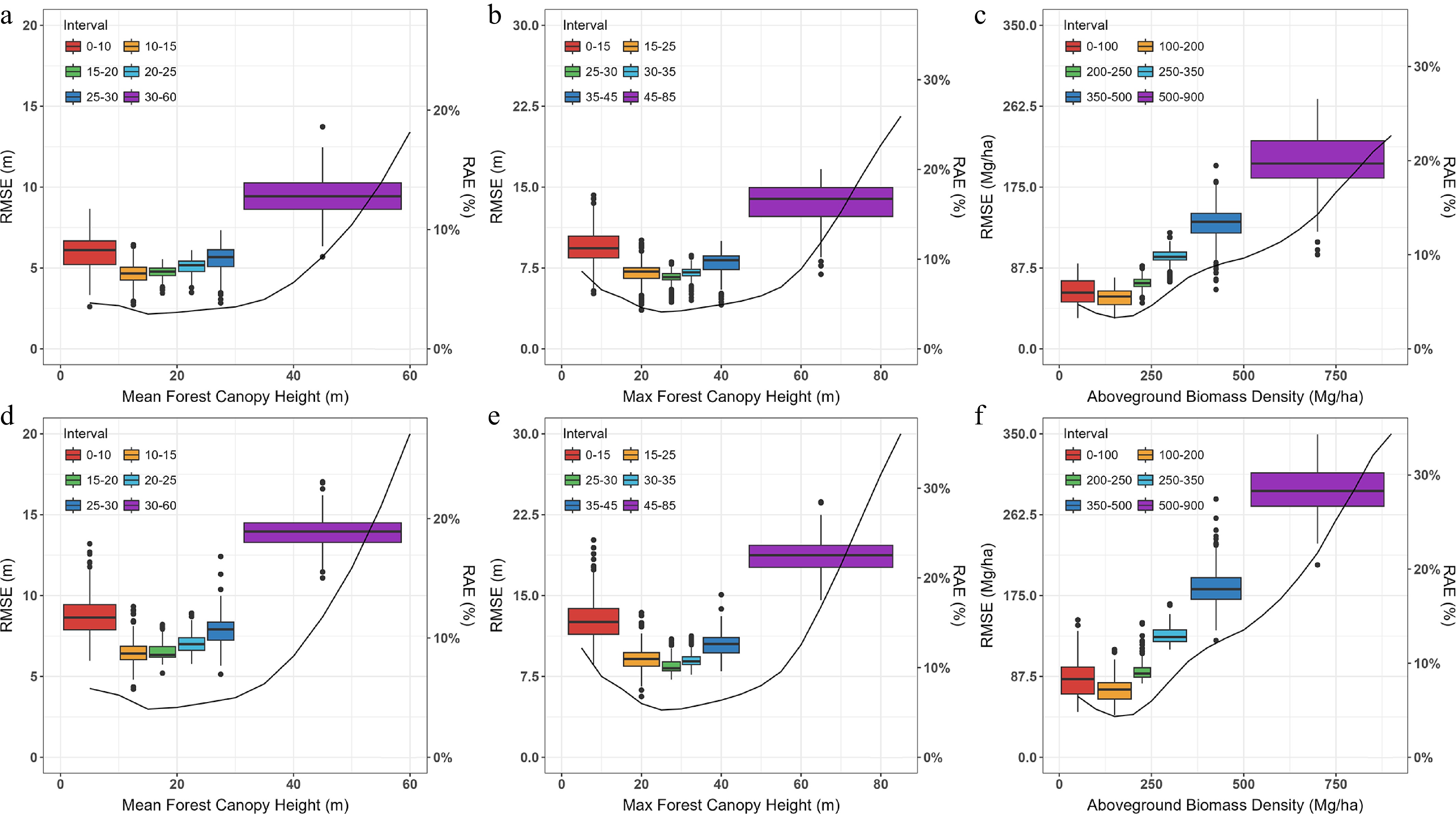
Figure 6. 

Uncertainty within, and between estimation intervals for three forest parameters ([a] and [d] for mean FCH, [b] and [e] for max FCH, [c] and [f] for AGBD). (a)–(c), and (d)–(f) show the estimation accuracy of the training sets and test sets in each interval, respectively.

Model transfer from the training set to the test set remained relatively stable for mean FCH, particularly within the middle value range. In contrast, AGBD showed substantially larger uncertainty, with errors increasing rapidly toward higher biomass levels. This reflects the greater difficulty of establishing robust regression relationships for AGBD, partly because the available samples were concentrated within a limited value range, and partly because biomass variation is more weakly expressed in the predictor space than canopy height.

Product comparison

To assess the effectiveness of forest parameter estimation, we compared with existing forest parameter maps resulting from research in China or on a global scale. Table 5 presents information on the different forest parameter products. Current researchers have only focused on estimating max FCH and AGBD. However, this study also explored the ability to estimate mean FCH, further expanding the potential of LiDAR to express vertical information about forests, which has received less attention than maximum height or biomass. Therefore, this section only compares products for max FCH and AGBD. Existing products (Table 5) were developed using different strategies, including microwave-based semi-empirical modeling and machine-learning approaches, combining field measurements with multisource predictors such as canopy height, spectral indices, topographic variables, climate, and soil properties. These differences in data sources and modeling strategies provide an important context for evaluating the relative strengths of the proposed products. Regardless of the modeling or characterization used in these studies, the core issue is to regress forest structural characteristics on Earth observation data. These methods showed good performance throughout China, and globally; (AGBD R² = 0.49~0.67, RMSE = 56.28~70.71 Mg/ha; max FCH R² = 0.55~0.62, RMSE = 5.3~7.3 m). Nevertheless, different methods showed significant variations in high forest coverage regions.

Aboveground biomass density

Compared to the proposed map, other maps (Fig. 7a–c) were underestimated to varying degrees (μ > 100 Mg/ha). We used the 99^th quantile of AGBD as the saturation points. Other maps cannot provide a complete expression of AGBD interval distribution with lower saturation points (634.6 Mg/ha in the proposed map, 191.4 Mg/ha in the Santoro map, 160.1 Mg/ha in the Zhang map, and 131.4 Mg/ha in the Yang map). Based on GEDI measurements (Fig. 8a−d), compared to the proposed map (R = 0.78, RMSE = 136.18 Mg/ha, Bias = –41.22 Mg/ha), other maps have a strong saturation effect, which leads to essentially no linear relationship with GEDI L4A products (R < 0.1, RMSE > 200 Mg/ha, Bias < –150 Mg/ha). Based on survey data, other maps (RMSE > 99.96 Mg/ha, RAE > 65.3%, Bias < –75.59 Mg/ha) show greater uncertainty than proposed map (RMSE = 81.00 Mg/ha, RAE = 52.8%, Bias = –36.50 Mg/ha) in Table 6. The proposed method has been greatly improved compared to other results.

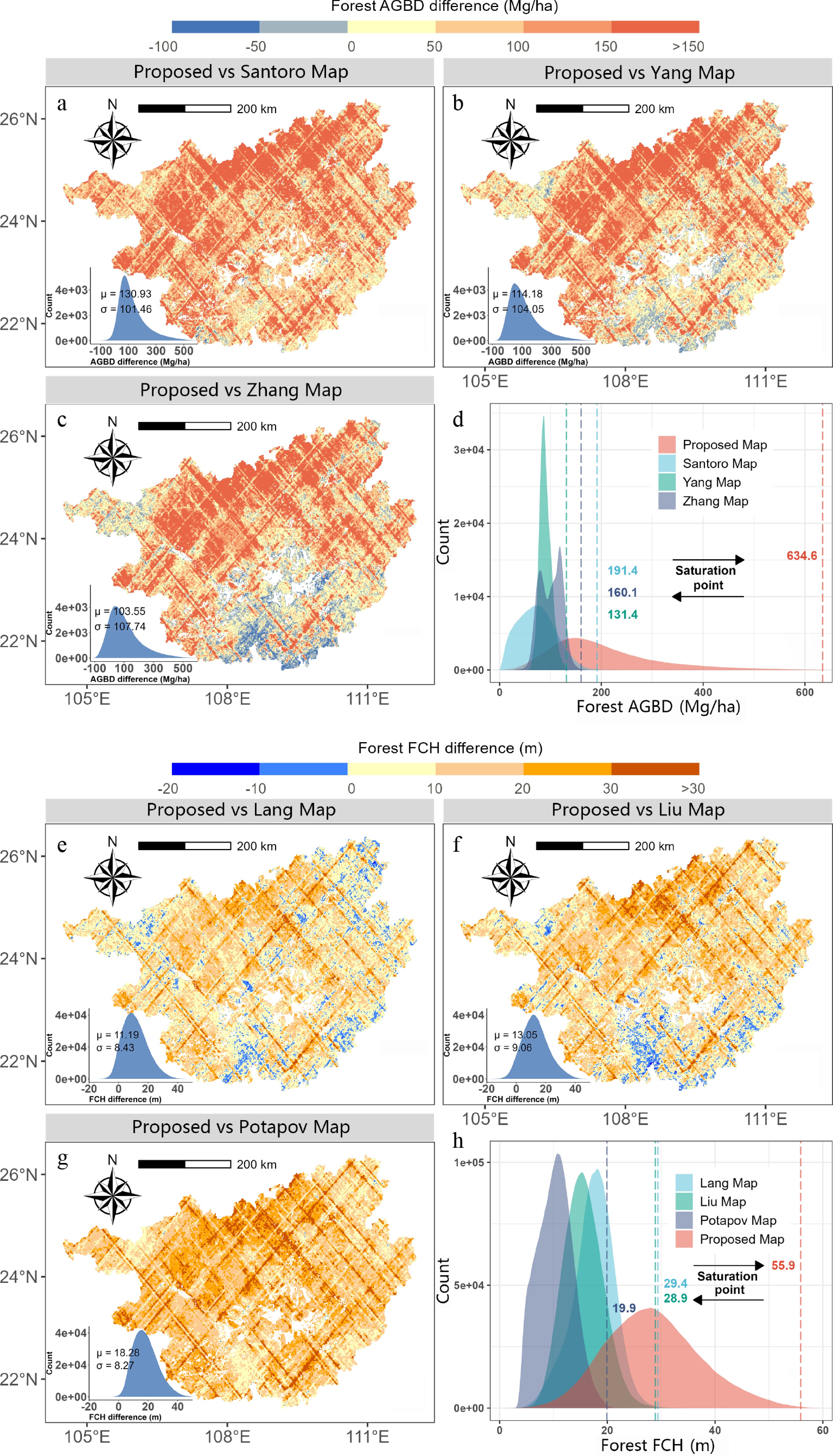
Figure 7. 

(a)–(c) Differences between the proposed AGBD mapping result and other products. (d) The AGBD distribution of each product. (e)–(g) Differences between proposed max FCH mapping result and other products. (h) Max FCH distribution of each product.

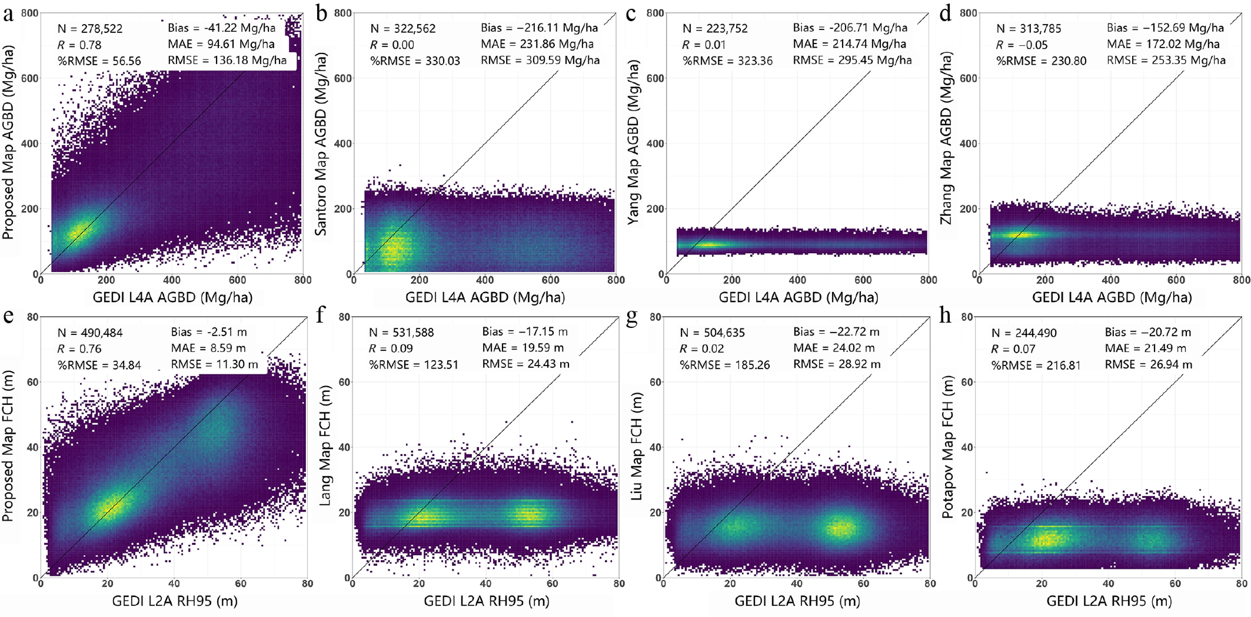
Figure 8. 

(a)–(d) Scatter plots between the GEDI L4A footprint product and the four AGBD map types. (e)–(h) Scatter plots between the GEDI L2A RH95 height footprint products and the four max FCH maps.

Max forest canopy height

Other maps (Fig. 7e–g) showed underestimation (μ > 10 m) compared to our product. Other maps cannot provide a complete expression of the max FCH interval distribution with lower saturation points (55.9 m in the proposed map, 29.4 m in the Lang map, 28.9 m in the Liu map, and 19.9 m in the Potapov map). GEDI L2A RH95 samples greater than 30 are numerous. Based on GEDI measurements (Fig. 8e−h), compared to the proposed map (R = 0.76, RMSE = 11.30 m, Bias = –2.51 m), other maps have a strong saturation effect, which leads to essentially no linear relationship with GEDI L4A products (R < 0.1, RMSE > 20 m, Bias < –15 m). Based on survey data, other maps (RMSE > 9.27 m, RAE > 49.2%, Bias < –4.45 m) show greater uncertainty than proposed map (RMSE = 7.21 m, RAE = 38.2%, Bias = −2.99 m) in Table 6. The proposed method has been greatly improved compared to other results. Max FCH estimation (RMSE = 34.84) shows a more robust regression than AGBD (RMSE = 56.56).

As the results of this study have shown, the method of training machine learning models using GEDI forest parameters based on spectral information directly produces a strong banding response^[58]. While the use of other interpolation methods may reduce this problem, this would not fundamentally solve the saturation effect. The observed systematic underestimation in existing biomass/height maps is particularly pronounced in high-value regions. Primarily, widespread reliance on optical vegetation indices leads to signal saturation in dense, multi-layered canopies. Furthermore, coarser spatial resolutions in some products smooth over fine-scale structural heterogeneity, resulting in generalized, lowered averages where local variability is high.

This study built relationships between GEDI products and Landsat8 features based on the AutoML method, and implemented forest parameters (including mean FCH, max FCH, and AGBD) mapping over a large region. Firstly, we found that RH55 (RMSE = 5.63 m) and RH95 (RMSE = 7.21 m) are the most suitable for modeling the mean and max FCH models, while the estimation RMSE of AGBD was 81.0 Mg/ha in the survey area. Then, the relationships between LiDAR response and forest parameters are extended to the entire Guangxi region. Compared with other methods (such as DeepL), AutoML can improve the accuracy by at most 3.93 m, 5.53 m, and 51.18 Mg/ha for mean FCH, max FCH, and AGBD parameters, respectively. One notable finding is the significant contribution (over 50%) of the FOTO feature among numerous features in the modeling process. The inclusion of the FOTO feature noticeably enhances the linear trend (R² improved by approximately 0.28 in mean FCH, 0.26 in max FCH, and 0.34 in AGBD) observed in the model.

Compared to other maps, the proposed map reduced the spectral saturation problem, showing greater correlation with GEDI estimates, especially at high values of height and biomass. For AGBD, correlation with GEDI showed R = 0.78 and RMSE 136 Mg/ha for the proposed map, compared to typical values of R < 0.1 and RMSE in the range 253–309 Mg/ha for the three others compared. Based on survey data, the proposed map (RMSE = 81.00 Mg/ha, RAE = 52.8%, Bias = –36.50 Mg/ha) showed less uncertainty than other maps (RMSE > 99.96 Mg/ha, RAE > 65.3%, Bias < –75.59 Mg/ha).

This framework integrates globally available GEDI LiDAR, multi-sensor satellite imagery, an automated, data-driven modeling workflow—it is inherently designed for transferability. The methodology does not rely on region-specific empirical adjustments. Its reliance on physically interpretable, multi-scale features and an adaptive AutoML engine suggests strong potential for application across other forest biomes and geographic regions. Future work will focus on testing this scalability across diverse continental and global forest ecosystems.