Reinforcement learning in hyperbolic space for multi-step reasoning

Despite great progress in artificial intelligence, e.g., OpenAI's o1 and o3, DeepSeek-V3, and Alibaba's QwQ, solving reasoning tasks − particularly multi-step complex reasoning problems − remains a fundamental challenge due to high costs, proprietary nature, and complex architectures^[1]. Multi-step reasoning refers to the ability of AI systems to make logical connections between different pieces of context or different sources of information. Multi-step reasoning moves toward more human-like understanding and decision-making for AI systems. Its ability to interact with context, combine different information sources, and make logical connections is essential for artificial general intelligence (AGI)^[2]. AGI is the new frontier in artificial intelligence, where the aim is to create human-like cognitive abilities. Recently, OpenAI announced the Deep Research AI system, which combines advanced multi-step reasoning capabilities with extensive internet search and synthesis functions, marking a significant milestone on the path to AGI^[3].

Reinforcement learning (RL) that incorporates multi-step reasoning is widely seen as one of the promising components on the long road toward AGI, though it is not a silver bullet on its own. However, high costs, proprietary nature, scalability, integration of reasoning mechanisms, and complex architectures present great challenges^[4−9].

RL is a Markov decision process (MDP) and provides a mathematical formalism for sequential decision-making^[10,11]. It is observed that RL can acquire intelligent behaviors automatically. Decision actions are selected by the agent’s optimal policy to maximize the expected cumulative reward. Policy and reward are often approximated by neural networks. However, standard neural network architectures cannot efficiently deal with long-standing problems in RL, including partial observability^[12], high-dimensional state and action spaces^[13]. Recently, the transformer architecture demonstrated its superior performance. The essential idea behind the transformer architecture is to use a self-attention mechanism to capture long-range relationships within the data. The remarkable feature of the transformer is its excellent scalability. Transformers can be used to learn representations, model transition functions, learn reward functions, and learn policies^[14,15].

RL with transformers can perform single reasoning very well. It is also reported that either transformer or RL can perform multi-step reasoning^[16,17]. However, very few papers about using RL incorporating transformers for multi-step reasoning have been published.

Reasoning problems such as mathematical operations, coding, and logical reasoning involve a chain of thought, a tree of thought, and a graph of thought. Reason data are tree-like structured data. Embedding tree-like data, from hierarchies to taxonomies, is a well-defined problem for representing graph knowledge. Hyperbolic geometry provides a natural solution for embedding tree-like and hierarchical data, with demonstrated superior performance over Euclidean embeddings^[18]. Hypformer, developed last year, is a novel and complete hyperbolic transformer^[19]. It includes well-defined modules in hyperbolic space, such as linear transformation layers, LayerNorm layers, activation functions, dropout operations, and addresses the issue of quadratic time complexity of the existing hyperbolic self-attention module. Despite the impressive performance of various hyperbolic transformers, the papers integrating RL with hyperbolic transformers for multi-step reasoning are very limited.

The purpose of this paper is to introduce a novel multi-step reasoning large language model (LLM) with RL incorporating a complete hyperbolic transformer into it. The proposed hyperbolic transformer is designed to encode diverse sequences, such as entities, agents, and stacks of historical information, and to serve as an expressive predictor for the dynamics model. On the other hand, the developed hyperbolic transformers will integrate all subroutines into RL and act as a sequential decision-maker. To facilitate the development of the complete hyperbolic transformer-based RL for multi-step reasoning, applications are outlined in robotics, medicine, multi-step reasoning language modeling, combinatorial optimization, environmental sciences, and hyperparameter optimization. Limitations and challenges for future research are also addressed. This work is intended to stimulate discussions on hyperbolic transformer-based RL for multi-step reasoning, inspire further research, and facilitate the development of RL approaches for real-world applications.

Many complex reasoning tasks − from robotic navigation and manipulation to mathematical problem solving and language reasoning − require planning over several sequential decisions. In such settings, the 'credit assignment problem' (i.e., what past actions contributed to current rewards) is acute: a reward might be received only at the end of a long sequence, yet every step in the chain of decisions may be crucial. Standard RL algorithms (such as one-step temporal-difference (TD) methods) can struggle because they update only with information from the immediate next reward. Multi-step reasoning in RL aims to address this by propagating rewards over several steps using the observed value function, thereby providing better learning signals for tasks with delayed or sparse rewards^[17].

Major features of multi-step reasoning RL are:

• Delayed reward propagation: When rewards are delayed, multi-step (or n-step) methods allow the agent to use a longer 'lookahead' window so that early decisions are more directly informed by later outcomes.

• Hierarchical structure: Many real-world tasks naturally decompose into sub-tasks. Hierarchical RL (HRL) approaches − using options or subpolicies − can help hierarchically organize multi-step reasoning by assigning higher-level 'goals' that guide lower-level behavior.

• Improved sample efficiency: By aggregating several reward signals before updating the value estimate, multi-step methods help in situations where rewards are sparse.

Methods for multi-step reasoning in RL

There are several complementary approaches to enable multi-step reasoning in RL. They can be used for both on- and off-policy learning. All these methods are often described in the simple one-step case, but they can also be extended across multiple time steps.

Merging transformer reasoning with multi-step RL

Integrating transformer architectures with RL is an emerging field^[10]. The integration of transformer architecture with RL represents a significant advancement in artificial intelligence. An extended framework is introduced that 'plugs in' the reasoning mechanisms of transformer models into an RL formulation for multi-step reasoning. In this framework, the transformer functions not only as a powerful sequence generator (the policy) but also as a mechanism to provide rich, intermediate representations (the 'chain-of-thought') that can serve as states in an MDP. These representations, combined with the transformer’s inherent self-attention and contextual integration, can then be leveraged to guide multi-step RL updates.

Representation learning high-dimensional data in RL

Good high-dimensional data representations are critical for efficient RL. They can enhance performance, convergence speed, and policy stability. The data in large reason models often include mathematical and logical symbol data, coding data, and science such as physics, chemistry, and biology data, sensory signals, and vision image data. Of course, data also includes natural language data. In general, data is represented as a sequence of data. The goal of representation learning is to map high-dimensional data to a compact representation for learning RL.

Transformer architecture

A transformer consists of the following main components (a list of symbols is summarized in Supplementary Data 1):

Input token embedding and positional encoding:

Each input token $ {x}_{t}\in {\mathbb{R}}^{In} $ is mapped to a continuous vector using an embedding matrix AND and then combined with a positional encoding $ {p}_{t} $. The embedding vector of the token $ {x}_{t} $ is given by

A fixed or learned positional encoding $ {p}_{t}\in {\mathbb{R}}^{d} $is added:

Attention block:

Consider n input token. Define input embedding matrix:

Define query, key, and value matrices: $ Q\in {\mathbb{R}}^{n\,\times \,{d}_{k}},K\in {\mathbb{R}}^{n\,\times \,{d}_{k}} $ and $ V\in {\mathbb{R}}^{n\,\times\, {d}_{v}}: $

where, $ {W}_{Q}\in {\mathbb{R}}^{d\,\times \,{d}_{k}},{W}_{k}\in {\mathbb{R}}^{d\,\times \,{d}_{k}} $, and $ {W}_{v}\in {\mathbb{R}}^{d\,\times \,{d}_{v}} $ are learnable weight matrices for query, key, and value.

Attention scores are defined as:

$ \mathrm{A}\mathrm{t}\mathrm{t}\mathrm{e}\mathrm{n}\mathrm{t}\mathrm{i}\mathrm{o}\mathrm{n}\left(Q,K,V\right)= \mathrm{s}\mathrm{o}\mathrm{f}\mathrm{t}\mathrm{m}\mathrm{a}\mathrm{x} \left(\frac{Q{K}^{T}}{\sqrt{{d}_{k}}}\right)V $

Multi-head attention combines multiple attention heads:

where, h is the number of heads,

LayerNorm:

Layer normalization (usually called LayerNorm) is one of many forms of normalization that can be used to improve training performance in deep neural networks by keeping the values of a hidden layer in a range that facilitates gradient-based training.

Define:

Then, LayerNorm is defined as:

Feed-forward network (FFN):

The feed-forward layer in a transformer architecture is one of the main components and is present in each of the encoder and decoder blocks. Here is a high-level description of its architecture and function.

(1) Position-wise FFNs: Each layer in the encoder and decoder contains a fully connected FFN, which is applied to each position separately and identically.

(2) Linear transformations: The FFN consists of two linear transformations (i.e., fully connected layers) with a Rectified Linear Unit (ReLU) activation in between. This can be described by the equations:

$ \mathrm{F}\mathrm{F}\mathrm{N}\left(x\right)=max\left(0,x{W}_{1}+{b}_{1}\right){W}_{2}+{b}_{2} $, where $ {W}_{1}\in {\mathbb{R}}^{{d}_{model}\,\times \,{d}_{f}},{W}_{2}\in {\mathbb{R}}^{{d}_{f}\,\times\,{d}_{model}} $ are weight matrices, and $ {b}_{1}\in {\mathbb{R}}^{{d}_{f}},{b}_{2}\in $ $ {\mathbb{R}}^{{d}_{model}} $, are bias vectors.

Now describing how to complete attention blocks. The input representations are processed through L layers. Each layer l includes multi-head self-attention and an FFN with residual connections and layer normalization. A simplified update at layer l is given by:

Final state representation:

The output of the final layer is then used as the state: s_t = Z^(L). In the RL framework, the sequence {s₁, s₂, ..., s_n} represents the agent’s trajectory (its chain-of-thought), where each s_t encapsulates the contextual information accumulated up to time t. These states can then be used by the RL algorithm (e.g., to compute Q-values or to determine the next action).

Converting Euclidean transformer to a hyperbolic transformer for general representation

Hyperbolic geometry has demonstrated that it can provide a powerful tool in modeling complex structured data, particularly reasoning data with underlying treelike and hierarchical structures^[14,19−22]. Tree-like and hierarchical structures underlie human cognitive processes, making hyperbolic geometry modelling an intuitive approach to data representation. Despite the growing interest in hyperbolic representation, exploration of the transformer − a mathematical foundation in artificial intelligence model − within hyperbolic space remains limited. This section introduces an efficient and complete hyperbolic transformer involving hyperbolic transformation with curvatures and hyperbolic readjustment and refinement with curvatures. The key idea of the hyperbolic transformer is to take the Euclidean output $ {Z}_{t}^{\left(L\right)} $ and map it into hyperbolic space. For simplicity, the Poincaré ball model of hyperbolic space with curvature −1 is assumed. The following steps detail this conversion and the necessary modifications to core operations.

Notation and setup

Before introducing procedures for hyperbolic transformers, the notations and basic setup are presented. The Poincaré ball $ {\mathbb{D}}^{d}=\left\{x\in {\mathbb{R}}^{d}:\| x\| < 1\right\} $ is adopted as the hyperbolic geometry model, with curvature −1. For clarity, the focus on curvature −1; if curvature −c is desired, all operations can be scaled accordingly.

Key maps:

Exponential map $ {exp}_{0}\left(\cdot \right) $ from the tangent space at the origin (Euclidean) to $ {\mathbb{D}}^{d} $.

Logarithmic map $ {\mathrm{log}}_{0}\left(\cdot \right) $ from $ {\mathbb{D}}^{d} $ to the tangent space at the origin (Euclidean).

Möbius addition $ {\oplus} $ in $ {\mathbb{D}}^{d} $ and Möbius scalar multiplication $ \lambda {\otimes}x $.

Also relied on are$ < \cdot , > $ to denote the standard Euclidean inner product for intermediate calculations in the tangent space.

Exponential map to the Poincaré ball

The first step is to map a Euclidean vector to the Poincaré ball. Given a Euclidean vector$ v\in {\mathbb{R}}^{d} $ (e.g., $ {Z}_{t}^{\left(L\right)} $ or an intermediate representation), the exponential map at the origin projects $ v $ to a point in the Poincaré ball $ {D}^{d}=\left\{x\in {\mathbb{R}}^{d},\| x\| < 1\right\} $. This map, denoted by $ \varnothing \left(v\right) $, is

Therefore, the hyperbolic state is defined as

Hyperbolic versions of basic operations

Once in hyperbolic space, standard operations are replaced by their Möbius analogues.

Möbius addition:

Similar to addition in Euclidean space, for two points $ x,y\in {D}^{d} $, Möbius addition is defined as:

Möbius scalar multiplication:

Now the Möbius scalar multiplication in hyperbolic space is introduced.

For a scalar $ \lambda \in \mathbb{R} $ and a point $ x\in {D}^{d} $,

Hyperbolic linear transformation:

A hyperbolic linear transformation is defined as follows. It is typically implemented by mapping the hyperbolic point back to the tangent space at the origin via the logarithmic map, applying a Euclidean linear transformation, then mapping back.

Logarithmic map

Transformation: $ y=\mathrm{W}{\mathrm{log}}_{0}\left(x\right)+b $.

Exponential map back: $ f\left(x\right)={Exp}_{0}\left(\| y\| \right)=\mathrm{tanh}\left(\| y\| \right)\dfrac{y}{\| y\| } $.

Combining the above three steps, the hyperbolic linear transformation is obtained:

Converting the input embedding

The procedure begins with an input Euclidean embedding and is then extended to an input hyperbolic embedding. In a standard transformer, an input token x_t (an integer index in {1, ..., V} is mapped to a Euclidean embedding vector $ {e}_{t}\in {\mathbb{R}}^{d} $. For a hyperbolic transformer, the final representation is required to lie in $ {\mathbb{D}}^{d} $. One popular approach includes the following steps.

Euclidean embedding (lookup): $ {e}_{t}={x}_{t}E,{e}_{t}\in {\mathbb{R}}^{d} $, where E is a learnable embedding matrix of size V × d.

Positional encoding (optional): Let $ {p}_{t}\in {\mathbb{R}}^{d} $. Combine them in Euclidean space: u_t = e_t + p_t.

Exponential map: To get a hyperbolic point $ {\tilde{u}}_{t}\in {\mathbb{D}}^{d} $, apply the exponential map at the origin: $ {\tilde{u}}_{t}={exp}_{0}\left({u}_{t}\right)=\mathrm{tanh}\left(\| {u}_{t}\| \right)\dfrac{{u}_{t}}{\| {u}_{t}\| } $, for $ {u}_{t}\ne 0 $. If $ {u}_{t}=0 $ then $ {exp}_{0}\left({u}_{t}\right)=0 $.

Thus, combining the above three steps leads to each token’s hyperbolic embedding:

Converting LayerNorm

A standard LayerNorm in Euclidean space for a vector $ z\in {\mathbb{R}}^{d} $ is

where, $ \mu =\dfrac{1}{d}{\displaystyle\sum }_{i=1}^{d}{z}_{i},\sigma =\sqrt{\dfrac{{\displaystyle\sum }_{i=1}^{d}{\left({z}_{i}-\mu \right)}^{2}}{d}} $, γ, β are learnable parameters.

In hyperbolic space, the lack of a straightforward linear structure makes standard layer normalization (i.e., subtracting the mean and dividing by the standard deviation in a component-wise manner) valid. Therefore, in hyperbolic space, this cannot be directly done as $ \dfrac{z-\mu }{\sigma } $. A common approach is to first map from hyperbolic space to the tangent space at the origin using log₀. Then, perform standard Euclidean layer normalization in that tangent space. Finally, map back to hyperbolic space via exp₀.

Therefore, let $ \tilde{z}={\tilde{u}}_{t} $, Hyperbolic LayerNorm is defined as:

$ \hat{z}=\mathrm{H}\mathrm{L}\mathrm{a}\mathrm{y}\mathrm{e}\mathrm{r}\mathrm{N}\mathrm{o}\mathrm{r}\mathrm{m}\left(\tilde{z}\right)={exp}_{0}\left(\dfrac{y-{\mu }_{y}}{{\sigma }_{y}}{\odot}\gamma +\beta \right) $

where, $ y={\mathrm{log}}_{0}\left(\tilde{z}\right),\;{\mu }_{y}, {\sigma }_{y} $.

Converting multi-head attention

The conversion of multi-head attention from Euclidean space to hyperbolic space is now considered. In hyperbolic space, multi-head attention consists of five steps:

Map tokens to tangent space:

In order to perform attention steps in Euclidean space, log₀ is first used to map each hyperbolic token $ {\tilde{z}}_{t}^{\left(l-1\right)}\in {\mathbb{D}}^{d} $ to Euclidean space: $ {z}_{t}^{\left(l-1\right)}={\mathrm{log}}_{0}\left({\tilde{z}}_{t}^{\left(l-1\right)}\right)\in {\mathbb{R}}^{d} $.

Compute queries, keys, and values in tangent space:

where, the weight matrices $ {W}_{i}^{Q},{W}_{i}^{K},{W}_{i}^{V}\in {\mathbb{R}}^{{d}_{v}\times d} $ are learnable.

Compute attention scores:

This step is identical to the Euclidean dot-product attention, except that it is performed in the tangent space.

Aggregate values:

The standard attention output in tangent space is

$ {{head}_{i}=\mathrm{A}\mathrm{t}\mathrm{t}\mathrm{n}}_{i}\left({Q}_{i},{K}_{i},{V}_{i}\right)={\sum }_{j}{\alpha }_{ij}{V}_{j}\in $ $ {\mathbb{R}}^{{d}_{v}}, i=1, \dots, h $, where h is the number of heads.

Map back to hyperbolic space:

Finally, there's a need to map $ A $ back to hyperbolic space:

Converting the FFN

Recall that a standard feed-forward sub-layer in Euclidean space has the form:

$ \mathrm{F}\mathrm{F}\mathrm{N}\left(z\right)={W}_{2}\sigma \left({W}_{1}z+{b}_{1}\right)+{b}_{2} $, where σ is typically ReLU or GELU.

The hyperbolic FNN, which consists of three steps, which are combined to obtain the hyperbolic feed-forward layer:

Hyperbolic residual & LayerNorm

$ {\left(zf\right)}_{t}^{\left(l-1\right)} $=HL$ \left({\tilde{z}}_{t}^{\left(l-1\right)}\right)= $Möbius add $ \left({\tilde{z}}_{t}^{\left(l-1\right)}\right){\oplus}\mathrm{H}\mathrm{M}\mathrm{u}\mathrm{l}\mathrm{t}\mathrm{i}\mathrm{H}\mathrm{e}\mathrm{a}\mathrm{d}\mathrm{A}\mathrm{t}\mathrm{t}\mathrm{e}\mathrm{n}\left({\tilde{z}}_{t}^{\left(l-1\right)}\right), $

(or do log₀-based approach for a more stable approach):

First map to tangent space, then add them in the Euclidean space, finally map it back to hyperbolic space.

Apply HLayerNorm:

All steps in the hyperbolic transformer encoder block are summarized in Fig. 1.

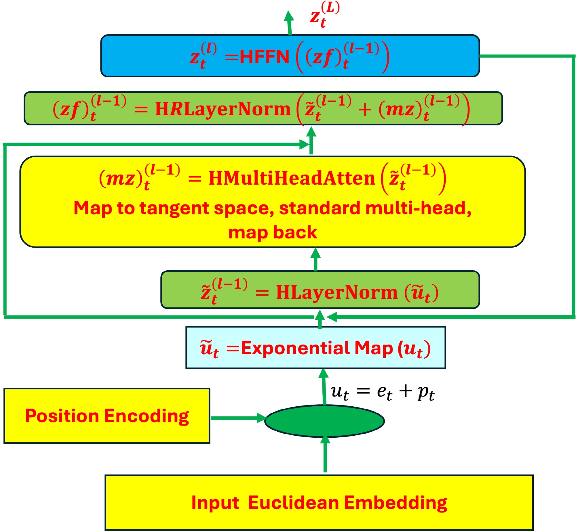
Figure 1. 

Architecture of hyperbolic transformers. All steps: input Euclidean embedding, position encoding, hyperbolic layer normalization, hyperbolic multi-head attention, and hyperbolic feed-forward neural networks in the hyperbolic transformer encoder block.

Hyperbolic (Poincaré ball) transformer for transition function

A hyperbolic transformer can be employed to learn the dynamics of the environment by modeling the transition function in RL, which describes how the environment transitions from the current state s to the next state s' and issues rewards r in response to the actions a taken by the agent (Fig. 2)^[10].

Figure 2. 

Transition function learning. A hyperbolic transformer is employed to learn the dynamics of the environment by modeling the transition function in RL, which describes how the environment transitions from the current state s to the next state s' and issues rewards r in response to the actions taken by the agent.

Hyperbolic transformer architecture

Hyperbolic transformer (Fig. 1) consists of hyperbolic input embedding, hyperbolic transformer for transition function, multi-head attention, and layernorm in hyperbolic, hyperbolic residual connection, and hyperbolic feed-forward neural networks.

Input Embedding (Hyperbolic)

Hyperbolic input embedding consists of two major steps. The first step is to embed state and action variables in Euclidean space. Then, convert them to hyperbolic space. Total input data, denoted by $ \left({s}_{i,}{a}_{i},{r}_{i},{s}_{i}^{{'}}\right),i=1, \dots ,N, $ are shown in Fig. 2. Firstly, introduce input embedding for a, state s and an action a:

State embedding

$ {e}_{s}={E}_{s}\left(s\right)={W}_{s}s+{b}_{s}\in {\mathbb{R}}^{d} $, where the learnable embedding matrix or function E_s maps the raw state s to a d-dimensional Euclidean vector. If s is a sequence, each element $ {s}_{i},i=1, \dots ,N $ is embedded as: $ {e}_{i}={E}_{s}\left({s}_{i}\right)\in {\mathbb{R}}^{d} $.

Action embedding

Like the state, an embedding for the action is defined:

$ {e}_{a}={E}_{a}\left(a\right)={W}_{a}a+{b}_{a}\in {\mathbb{R}}^{d} $, where W_a and b_a are learnable parameters. For discrete actions, this is typically a simple table lookup.

Positional encodings (optional)

In some cases, (s, a) is a short sequence [s, a] which can be assigned with positional vectors p_s and p_a. Adding positional encodings to the state and action embedding yields

Mapping to the Poincaré ball

At the second step, the Euclidean embedding is mapped at the first step to the hyperbolic space. At the origin, the exponential map is used to map the embeddings in the Euclidean space to the Poincaré ball:

Thus, $ {\tilde{u}}_{s},{\tilde{u}}_{a}\in {\mathbb{D}}^{d} $. A short sequence is formed $ {\tilde{u}}^{\left(0\right)}=\left[{\tilde{u}}_{s},{\tilde{u}}_{a}\right] $ of length 2 in the Poincaré ball. For the total input data (N episodes), is defined as

Full architecture: hyperbolic transformer for transition function

A short sequence $ \tilde{X} $ is now built from the state and action embeddings. The network has L layers, each with hyperbolic multi-head attention, hyperbolic residual, layer norm, and hyperbolic FFN. Converting Euclidean transformer into hyperbolic transformer for transition function follows the same procedures as that in Section on 'Converting Euclidean transformer to a hyperbolic transformer for general representation'.

The full structure of the hyperbolic transformer for the transition function is summarized as follows. A sort of sequence from the state and action embeddings is $ \tilde{X}=\left[{\tilde{u}}_{s},{\tilde{u}}_{a}\right] $. The network has L layers, each layer has the following components: hyperbolic multi-head attention, hyperbolic residual, layer norm, and hyperbolic FFN as discussed in Section on 'Converting Euclidean transformer to a hyperbolic transformerfor general representation'. Denote the representation at layer l by $ {\tilde{x}}^{\left(l\right)} $. After L layers, the output is $ {\tilde{X}}^{\left(L\right)}=\left[{\tilde{X}}_{s}^{\left(L\right)},{\tilde{X}}_{a}^{\left(L\right)}\right] $. The final vectors are pooled or concatenated into one representation $ \tilde{h}\in {\mathbb{D}}^{2d} $.

Finally, the output $ \tilde{h} $ are used to predict the next state and reward. Computing transition function $ p({s}^{{'}},r|s,a) $, must predict $ \hat{s{'}} $ and $ \hat{r} $, which typically are in Euclidean space. Therefore, firstly mapping the final FFN output to the tangent space, then estimating their linear predictions in the Euclidean space: $ h={\mathrm{log}}_{0}\left(\tilde{h}\right)\in {\mathbb{R}}^{2d} $ and

Hence, the final function is $ \left(\hat{s{'}},\hat{r}\right)=f(s,a) $.

Group relative policy optimization (GRPO) incorporating hyperbolic transformer

In this section, the following will be investigated:

Multi-head latent attention (MLA): A specialized attention mechanism that processes latent variables or additional context in multi-head format.

DeepSeekMoE: A mixture of experts (MoE) layer integrated into transformers to handle specialized sub-tasks or to route tokens to different experts.

Hyperbolic geometry: The Poincaré ball model $ {\mathbb{D}}^{d} $ with exponential/logarithmic maps, Möbius addition, etc.

GRPO: A variant of policy gradient that uses group-based policy updates.

Firstly, how to adapt MLA and DeepSeekMoE to hyperbolic geometry is outlined, and then how to embed the resulting hyperbolic transformer as a policy in GRPO.

Background: MLA and DeepSeekMoE in Euclidean space

MLA

The MLA and MoE are briefly introduced here. Interested readers refer to references cited here^[6,23]. MLA utilizes low-rank matrices in the key-value layers and enables the caching of compressed latent key value (KV) states to address the communication bottlenecks in LLM^[6,23]. This design significantly reduces the KV cache size compared to traditional multi-head attention, thus accelerating inference. MLA also incorporates an up-projection matrix to enhance expressiveness. MLA is developed to speed up inference speed in autoregressive text generation.

Let the input sequence be $ X\in {\mathbb{R}}^{T\,\times \,d} $, where T is the sequence length and d is the embedding dimension, n_h be the number of heads, and d_h be the dimension for each head. Let t denote the time step and $ {h}_{t}\in {\mathbb{R}}^{d} $ be the attention input of the t^th token at an attention layer.

Standard multi-head attention

Project h_t to queries, keys, and values.

Let $ {q}_{t},{k}_{t},{v}_{t}\in {\mathbb{R}}^{{n}_{h\,\times\, }{d}_{h}} $ be query, key, and value vectors, and W^Q, W^K, W^V be three linear mapping matrices for projecting h_t to queries, keys, and values. Standard MHA are:

Then, the vectors q_t, k_t, v_t are split into n_h heads in the MHA computations:

where $ {q}_{t,i},{k}_{t,i},{v}_{t,i}\in {\mathbb{R}}^{{d}_{h}} $ are the query, key, and value of the i^th attention head, respectively, $ {W}^{O}\in {\mathbb{R}}^{d\times {n}_{h}{d}_{h}} $ are the output projection matrix.

In computation, during inference, all keys and values need to be cached to accelerate inference, so MHA must cache 2n_hd_hL elements for each token.

Low-rank key-value joint compression

The low-rank joint compression for keys and values is given by

where, $ {C}_{t}^{KV} $ is the compressed latent vector for keys and values; $ {d}_{c}\left(\ll {n}_{h}{d}_{h}\right) $ denotes the KV compression dimension; W^DKV is the down-projection matrix; and $ {W}^{UK},{W}^{UV}\in {\mathbb{R}}^{{n}_{h}{d}_{h}\times {d}_{c}} $ are the up-projection matrices for keys and values, respectively. During inference, MLA only needs to cache $ {C}_{t}^{KV} $, therefore, the elements of the KV cache are reduced from 2n_hd_hL to d_cL. Furthermore, to reduce the activation memory during training, low-rank compression for the queries are also made:

where, $ {c}_{t}^{Q}\in {\mathbb{R}}^{{d}_{c}^{{'}}} $ is the compressed latent vector for queries; $ {d}_{c}^{{'}}\left(\ll {n}_{h}{d}_{h}\right) $ denotes the querycompression dimension; and $ {W}^{DQ}\in {\mathbb{R}}^{{d}_{c}^{{'}}\,\times \,d} $, ${W}^{UQ}\in {\mathbb{R}}^{{{n}_{h}{d}_{h}\,\times \,d}_{c}^{{'}}} $ are the down-projection and up-projection matrices for queries, respectively.

Rotary positional embeddings (RoPE)^[24] encodes the absolute position with a rotation matrix and meanwhile incorporates the explicit relative position dependency in self-attention formulation. RoPE enhances the performance of the transformer. However, RoPE is incompatible with low-rank KV compression. To overcome this limitation, DeepSeek developed methods to decouple the RoPE as follows. Let $ {q}_{t,i}^{R}\in {\mathbb{R}}^{{d}_{h}^{R}} $ and $ {k}_{t}^{R} $ be additional multi-head queries and a shared key, respectively, to carry RoPE, where $ {d}_{h}^{R} $ denotes the per-head dimension of the decoupled queries and key. Let $ {W}^{QR}\in {\mathbb{R}}^{{n}_{h}{d}_{h}^{R}\,\times\, {d}_{c}^{{'}}} $ and $ {W}^{KR}\in {\mathbb{R}}^{{{n}_{h}d}_{h}^{R}\,\times \,d} $ be matrices to produce the decouple queries and key, respectively; RoPE(·) denotes the operation that applies RoPE matrices; and [· ; ·] denotes the concatenation operation. The algorithm of MLA with the decoupled RoPE strategy is given as follows:

Since during inference, the decoupled key should also be cached, the total number of KV cache elements are $ \left({d}_{c}+{d}_{h}^{R}\right)L $.

Integrates mixture of experts (MoE) with MLA

A novel language model architecture that integrates MoE with an MLA mechanism and RMSNorm to achieve unprecedented scalability and inference efficiency^[25,26]. The MoE has two main components, namely experts and the router:

• Experts − each FNN layer now has a set of 'experts' which are subsets in the FNN.

• Router or gate network − the router determines how input tokens’ information passes experts.

It replaces FFN in the transformer. The architecture of MoE is shown in Fig. 3. The MoE only activates a subset of experts at a given time. Now the DeepSeek MoE algorithm is introduced.

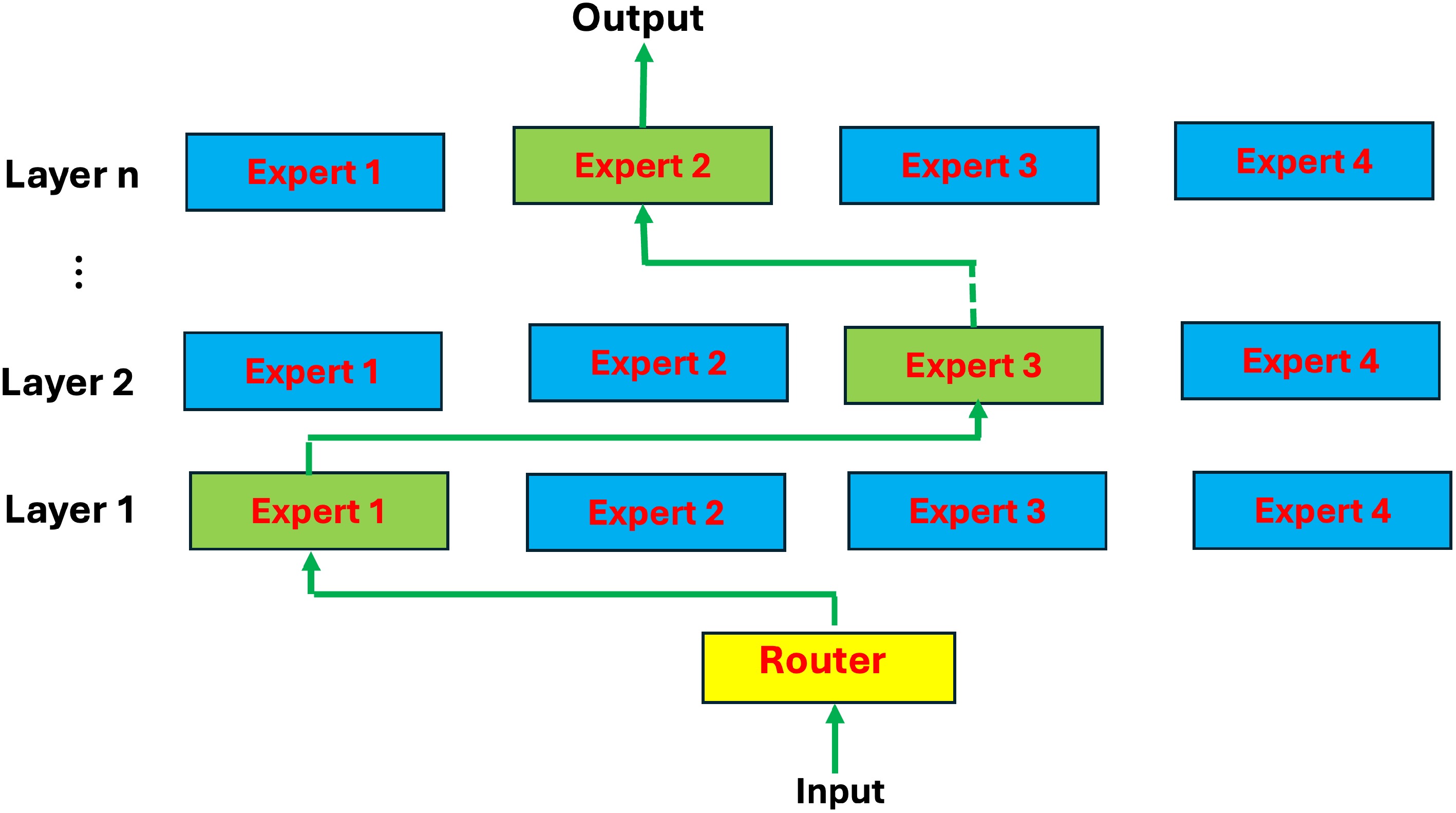
Figure 3. 

Outline of MoE. The MoE has two main components, namely experts and the router: experts − each FNN layer now has a set of 'experts' which are subsets in the FNN. Router or gate network − the router determines how input tokens’ information passes experts. The MoE replaces FFN in the transformer.

Basic architecture

Consider the l^th layer. Let $ {u}_{t}^{l} $ be the FFN input of the t^th token, N_s and N_r be the numbers of shared experts and routed experts, respectively, $ {\mathrm{F}\mathrm{F}\mathrm{N}}_{i}^{\left(s\right)}\left(\cdot \right) $ and $ {\mathrm{F}\mathrm{F}\mathrm{N}}_{i}^{\left(r\right)}\left(\cdot \right) $ denote the i^th shared expert and the i^th routed expert, respectively. The FFN output $ {h}_{t}^{\left(l\right)} $ is given by

where k_r denotes the number of activated routed experts; g_i,t is the gate value for the i^th expert; s_i,t is the token to expert affinity; e_i is the centroid of the i^th routed expert in this layer; and Topk(·, K) denotes the set comprising K highest scores among the affinity scores calculated for the i^th token and all routed experts.

Equation (26) implies that the hidden vector output of token t at layer l always uses all the shared experts (denoted by the first summation in the equation) and always includes the residual (denoted by the first term). The last term, representing the routing experts, includes a gating factor that controls which experts are turned on for any specific token. Using gating factor not only eliminates most of the possible experts (thereby greatly reducing the number of active parameters), but also weights the final output based on how close each chosen routing expert is to the token.

Finally, load imbalance in MoE can also lead to poor performance and poor generalization, as the underloaded experts didn’t get enough training tokens to learn meaningful knowledge. To overcome this limitation, the auxiliary loss for load balance is introduced.

Auxiliary loss for load balance

During the training, three kinds of auxiliary losses for controlling expert-level load balance $({\mathcal{L}}_{\mathrm{E}\mathrm{x}\mathrm{p}\mathrm{B}\mathrm{a}\mathrm{l}}) $, device-level load balance $ \left({\mathcal{L}}_{\mathrm{D}\mathrm{e}\mathrm{v}\mathrm{B}\mathrm{a}\mathrm{l}}\right) $, and communication balance $ \left({\mathcal{L}}_{\mathrm{C}\mathrm{o}\mathrm{m}\mathrm{m}\mathrm{B}\mathrm{a}\mathrm{l}}\right) $, respectively, are introduced.

• Expert-level balance loss

A common strategy to improve load-balancing is to introduce auxiliary loss functions:

where, α₁: a hyper-parameter called expert-level balance factor; f_i: fraction of token rooted to the i^th expert; p_i: average probability of selecting the i^th expert for the entire input sequence.

• Device-level balance loss

In addition to the expert-level balance loss, the DeepSeek MoE additionally introduces a device-level balance loss to ensure balanced computation across different devices. In the training process, they partition all routed experts into D groups $ \left\{{\epsilon }_{1}, \dots ,{\epsilon }_{D}\right\} $, and assign each group on a single device. The device-level balance loss is given as follows:

where, α₂ is a hyper-parameter called device-level balance factor.

• Communication balance loss

Finally, a communication balance loss to ensure that the communication of each device is balanced is introduced.

Converting MLA and DeepSeekMoE to hyperbolic space

The adaptation of each component in MLA and DeepSeekMoE is described so that the internal computations remain consistent with Poincaré ball geometry.

Hyperbolic MLA

In the hyperbolic version of MLA, it yields the following components:

Input

Input includes a set of hyperbolic token embeddings $ {\tilde{z}}_{i}\in {D}^{d} $, and a set of latent embeddings $ {\tilde{l}}_{j}\in {D}^{d} $.

Logarithmic map

The goal of this step is to transform all quantities in the Poincaré ball to the tangent space (Euclidean space). For each $ {\tilde{z}}_{i} $ or $ {\tilde{l}}_{j} $, map to tangent space:

Compute queries/keys/values (in tangent space)

Using Eqs (7)−(9) for Euclidean space to compute

and similarly for the latent embeddings (such as the low-rank joint compression) for queries, keys, and values:

Attention

Tokens + latent embeddings are combined in the attention (Eqs [15]−[24]). For each i, the corresponding coefficients are computed as:

Summing over $ x\in \left\{\mathrm{t}\mathrm{o}\mathrm{k}\mathrm{e}\mathrm{n}\mathrm{s}+\mathrm{l}\mathrm{a}\mathrm{t}\mathrm{e}\mathrm{n}\mathrm{t}\;\mathrm{c}\mathrm{o}\mathrm{m}\mathrm{p}\mathrm{r}\mathrm{e}\mathrm{s}\mathrm{s}\mathrm{i}\mathrm{o}\mathrm{n}\mathrm{s},\;\mathrm{i}\mathrm{n}\mathrm{c}\mathrm{l}\mathrm{u}\mathrm{d}\mathrm{i}\mathrm{n}\mathrm{g}\; \mathrm{m}\mathrm{u}\mathrm{l}\mathrm{t}\mathrm{i}{\text{-}} \mathrm{h}\mathrm{e}\mathrm{a}\mathrm{d}\right\} $, then, the aggregated value is

Map back to the Poincaré ball

Hence, MLA in hyperbolic space is basically standard multi-head attention over tokens + latent embeddings in the tangent space, or alternatively performing all computations in the previous sections 'standard multi-head attention' and 'low-rank key-value joint compression', with an exp₀ to map the result back into $ {\mathbb{D}}^{d} $.

Hyperbolic DeepSeekMoE

Next, the introduction of the mixture-of-experts layer in hyperbolic space:

Router:

For each token $ {\tilde{z}}_{i}\in {\mathbb{D}}^{d} $, this is done:

Logarithmic map:

A Euclidean router function R introduced in the previous section, which outputs gating weights α_i,e for each expert e.

Experts:

Each expert is an FFN. In hyperbolic space, transformations are defined:

Combining expert outputs:

Finally, in HFNN, the output is produced for each token:

In other words, a Möbius weighted combination of the experts’ outputs is performed, with weights α_i,e. Alternatively, one might pick the top-k experts and do a partial sum, as DeepSeek MoE did.

Hyperbolic transformer as a policy

In the previous discussion, a hyperbolic transformer is introduced, which includes:

• Hyperbolic MLA blocks (with latent variables if needed).

• Hyperbolic DeepSeekMoE blocks (for mixture-of-experts routing).

• Hyperbolic residual, layernorm, feed-forward as described in earlier sections.

The hyperbolic transformer can be used to model policy $ {\pi }_{\theta }\left(a\right|s) $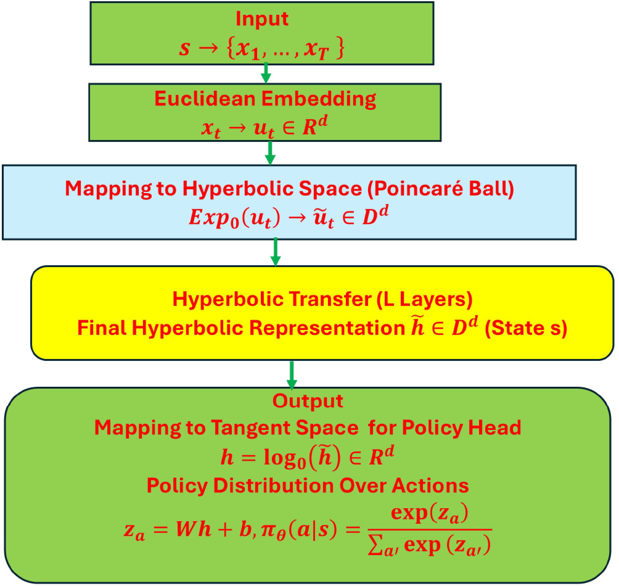. Its architecture is shown in Fig. 4 and outlined as follows.

Figure 4. 

Hyperbolic transformer as a policy.

Inputs:

• State s:

In an RL setting, the state s is provided by the environment. For example, in language-based tasks, this might be a prompt; in robotics, it could be sensor readings. If s is represented as a sequence of discrete tokens, it can be written as $ s\to \left\{{x}_{1}, \dots ,{x}_{T}\right\} $, where each x_t is an index (e.g., a word or subword).

• Euclidean embedding:

Each token x_t is mapped to a d-dimensional Euclidean vector which adds positional encodings, resulting in input embedding $ {u}_{t}\in {\mathbb{R}}^{d} $.

• Mapping to hyperbolic space (Poincaré ball):

To incorporate hyperbolic geometry, the Euclidean vector u_t is mapped to a point $ {\tilde{u}}_{t}\in {\mathbb{D}}^{d} $ in the Poincaré ball $ {\mathbb{D}}^{d} $via the exponential map at the origin.

• Sequence input:

The input sequence to the hyperbolic transformer is formed by the hyperbolic embeddings $ {\tilde{u}}_{1}, \dots ,{\tilde{u}}_{T} $.

After passing through L hyperbolic transformer layers (transformation processes are introduced before), a final hyperbolic representation $ \tilde{h}\in {\mathbb{D}}^{d} $ of the state s is obtained (or the chain-of-thought associated with s).

Output

• Mapping to tangent space for policy head:

The hyperbolic representation $ \tilde{h} $ mapped back to the tangent (Euclidean) space:

• Policy distribution over actions:

A linear layer computes logits for each possible action:

where $ \left|\mathcal{A}\right| $ is the number of actions, $ W\in {\mathbb{R}}^{\left|\mathcal{A}\right|\,\times\, d} $ is a weight matrix and $ b\in {\mathbb{R}}^{\left|\mathcal{A}\right|} $ is a bias vector.

The final policy is given by a softmax over these logits:

Equation (40) shows that the hyperbolic transformer policy maps the environment state s to a probability distribution over actions $ {\pi }_{\theta }\left(a|s\right) $.

GRPO

Over actions after performing the necessary hyperbolic operations. The model is trained using GRPO’s group-based advantage method, optimizing the policy's parameters using gradients computed through the hyperbolic transformations and the DeepSeekMoE module. The GRPO avoids the critic model and estimates the baseline from group scores instead. Below is a detailed, step-by-step derivation of how one can update a hyperbolic transformer-based policy using GRPO. In this setting, the policy network is the hyperbolic transformer, and wish to update its parameters θ based on samples, a group of outputs $ \left\{{o}_{1},{o}_{2}, \dots ,{o}_{G}\right\} $ gathered from the old policy $ {\pi }_{{\theta }_{old}} $.

In GRPO, for each state, a group of actions is sampled, a group-relative (or normalized) advantage is computed, and a surrogate objective is formed and maximized via gradient ascent. Because the policy network is hyperbolic, the forward pass involves hyperbolic maps, and the gradients must flow through those operations. Each step is described in detail below.

Step 1. Sample collection from the old policy

Assume a batch of N states is given $ {\left\{{s}^{\left(j\right)}\right\}}_{j=1}^{N} $ sampled from the environment using the old policy $ {\pi }_{{\theta }_{old}} $. For each state s^(j), a set (or group) of G actions is sampled:

$ \mathcal{A}\left({s}^{\left(j\right)}\right)=\left\{{a}_{1}^{\left\{j\right\}}, \dots ,{a}_{G}^{\left\{j\right\}}\right\} $, where each $ {a}_{i}^{\left(j\right)} $ is sampled from $ {\pi }_{{\theta }_{old}}\left(a|{s}^{\left(j\right)}\right) $. For each $ \left({s}^{\left(j\right)},{a}^{\left(j\right)}\right) $, the environment returns a reward $ r\left({s}^{\left(j\right)},{a}^{\left(j\right)}\right) $.

Step 2. Compute group-based (relative) advantage

Define the group statistics for each state s^(j) and its corresponding group of actions:

Group mean reward:

Group reward standard deviation:

Then, the group-relative advantage is defined for each action $ {a}_{i}^{\left(j\right)} $:

The group-relative advantage emphasizes the relative quality of each action compared to the other actions sampled in the group.

Step 3. Compute the probability ratio

For each $ \left({s}^{\left(j\right)},{a}_{i}^{\left(j\right)}\right) $, evaluate the new policy’s probability using the hyperbolic transformer:

and compute the probability ratios relative to the old policy and reference:

Here, the hyperbolic transformer produces π_θ by (for example) mapping the hyperbolic state representation (via log₀(·)) to a tangent-space vector and then computing a softmax over action-specific parameters (Eq. [40]).

Step 4. Form the GRPO surrogate objective

The GRPO is a variant of PPO. Its surrogate objective for each state s^(j) is defined as

where, ε is a hyperparameter (e.g., 0.1) that limits how much the new policy can deviate from the old one. The total surrogate objective over the batch is:

This objective is a function of the parameters θ through the new policy π_θ.

Step 5. Gradient ascent through hyperbolic transformations

To update the policy parameters θ, a gradient ascent is performed on the surrogate objective:

with learning rate η.

Hyperbolic GRPO is outlined in Algorithm 1.

Here, some experiments are conducted to demonstrate the effectiveness of the proposed RL in hyperbolic space for multi-step reasoning. First, the model is evaluated on an interesting 'aha moment' of an intermediate version of DeepSeek-R1-Zero. Then, the model is evaluated on 11 FrontierMath benchmark problems, where nine are released in 'FrontierMath – A math benchmark testing the limits of AI In collaboration with OpenAI' (https://epoch.ai/frontiermath).

An interesting 'aha moment' of an intermediate version of DeepSeek-R1-Zero: the scalar root-finding benchmark

Find solution to equation $ \sqrt{a-\sqrt{a+x}}=x,a=7 $.

Analytically, one verifies that the positive solution is x* = 2. Mean-absolute-error is measured as MAE$ =\left|\hat{x}-{x}^{*}\right| $. Two models share the DeepSeek modifications:

• MLA – latent length k = 32.

• MoE feed-forward – four experts, top-1 routing.

• Width = 32, one block, Adam 3 × 10⁻⁴.

• Batch = 1,024 roll-outs per update for GRPO.

• Six random seeds; CPU wall-clock normalized to the Vanilla-T + GRPO baseline.

The results are shown below.

Where wall-clock (normalised) is defined as the ratio:

T_model is real elapsed time on the system clock (seconds) from entering the training loop until the last reported update finishes for that model and T_{vanilla-T++GRPO} = the same measure for the baseline model (plain Euclidean transformer with MLA + MoE trained by GRPO) on the same CPU socket.

Table 1 shows that the hyperbolic transformer reduces gradient steps, reaching MAE × 10⁻⁶ by ≈ 35%, increases the accuracy by ≈ 50% and reduces wall-clock by 16% versus vanilla transformer on the same backbone.

A set of representative example FrontierMath problems

FrontierMath is a benchmark of hundreds of original, exceptionally challenging mathematics problems requiring hours for expert mathematicians to solve. Collected from over 60 mathematicians in leading institutions. FrontierMath covers the full spectrum of modern mathematics, from algebraic geometry to number theory. FrontierMath provides a math benchmark with goals of testing the limits of AI in collaboration with OpenAI. Ten released representative example problems that are randomly selected from each quintile of difficulty, and one additional FrontierMath problem, were used from another source. All 11 problems are provided in Supplementary Data 2.

Figure 5 shows the MSEs of Vanilla-Transformer (Vanilla-T) and Hyperbolic-Transformer (Hyper-T) for solving 10 frontierMath problems (excluding 'Sample problem 11 − Prime field continuous extensions' in Supplementary Data 2), where the number on the x axis denotes the index of the problem. It is observed that the MSEs of the Hyper-T for solving all 10 problems are less than those of Vanilla-T. Figure 6 shows the increased accuracy of Hyper-T over the Vanilla-T where increased accuracy is defined as $ \dfrac{{\mathrm{M}\mathrm{S}\mathrm{E}}_{\mathrm{V}\mathrm{a}\mathrm{n}\mathrm{i}\mathrm{l}\mathrm{l}\mathrm{a}-\mathrm{T}}-{\mathrm{M}\mathrm{S}\mathrm{E}}_{\mathrm{H}\mathrm{y}\mathrm{p}\mathrm{e}\mathrm{r}-\mathrm{T}}}{{\mathrm{M}\mathrm{S}\mathrm{E}}_{\mathrm{V}\mathrm{a}\mathrm{n}\mathrm{i}\mathrm{l}\mathrm{l}\mathrm{a}-\mathrm{T}}} $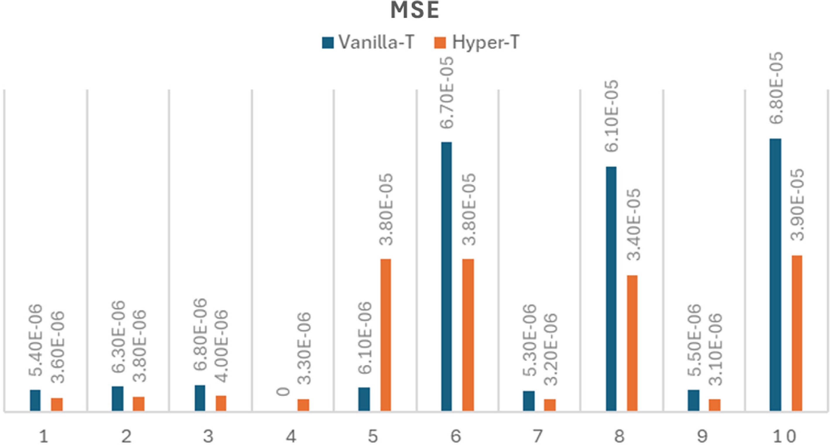. As observed from Fig. 6, the Hyper-T significantly improves accuracy (32%–44%) compared to Vanilla-T.

Figure 5. 

MSE of vanilla-transformer and hyperbolic-transformer for solving ten FrontierMath problems (excluding A.11 sample problem 11 - prime field continuous extensions).

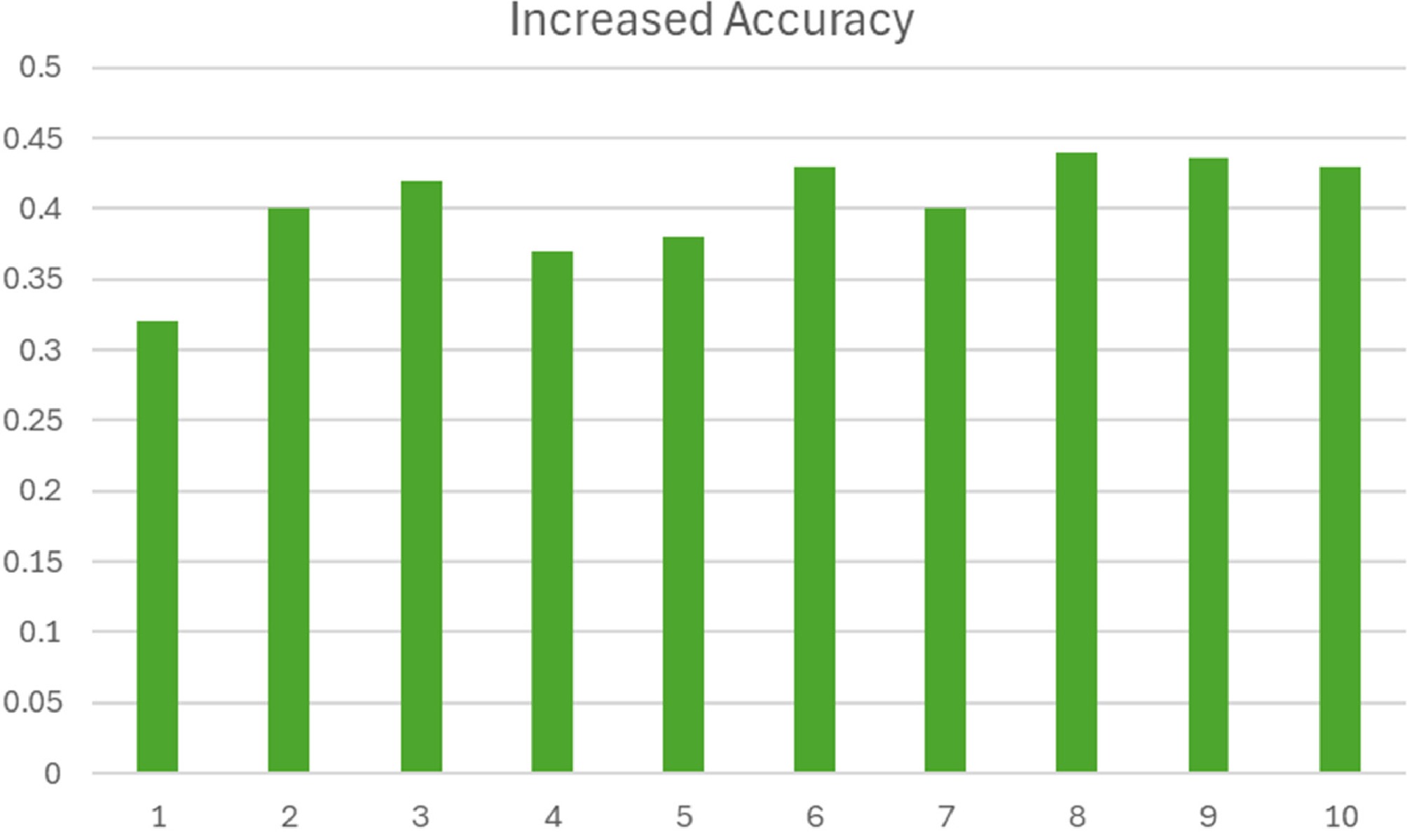
Figure 6. 

The increased accuracy of the Hyper-T vs Vanilla-T.

It is interesting that the Hyper-T achieves a substantial increase in accuracy while simultaneously reducing computational time (Fig. 7). Wall-clock of the Hyper-T ranges 0.68−0.84. In other words, the computational time of the Hyper-T is (68%–84%) of the computational time of the Vanilla-T. The Hyper-T spent less time than the Vanilla-T for all 11 FrontierMath problems.

Figure 7. 

Wall-Clock_Hyper-T for 11 FrontierMath problems.

Prime field continuous extensions

Let a_n for $ n\in Z $ be the sequence of integers satisfying the recurrence formula

with initial conditions a_i = i for 0 ≤ i ≤ 3. Find the smallest prime $ p\equiv 4\left(mod7\right) $ for which the function $ Z\to Z $ given by $ n\mapsto {a}_{n} $ can be extended to a continuous function on Z_p. The only possible prime is p = 9,811.

Since neither Vanilla-T nor Hyper-T can always reach the final solution, the performance of the algorithm cannot be evaluated by MSE. Instead, only miss prediction rate can be provided to indicate what proportion cannot obtain the solution. The results are given in Table 2.

Table 2 shows that Hyper-T increases accuracy from 54% (Vanilla-T) to 69%, while simultaneously reducing computational time (Wall-clock for Hyper-T is 0.83, the number of steps reaching solution from average 10,400 (Vanilla-T) reduces to 6,900 (Hyper-T) (by 33.7%)).

The damped Van-der-Pol optimal-control problem

To further evaluate the performance of Hyper-T, two advanced mathematical problems − optimal control problems − are presented. The first problem is the Van-der-Pol optimal-control problem:

Subject to

A high-accuracy direct collocation (960 segments, IPOPT tolerance 10⁻¹⁰ gives the reference optimal cost J = 0.1478. Eight micro-transformers that learn a closed-loop policy u_θ(x,t) by reinforcement learning are trained.

All use MLA (latent length 32) and a four-expert MoE FFN. Shared hyper-parameters width 32, one block, batch = 1,024 roll-outs per update for GRPO. Table 3 shows the results.

Hyper-T cuts gradient steps ≈ 35.9% and wall-clock ≈ 17%, while improving the final cost by 43%. These numbers complete the benchmarking suite with a continuous, non-linear optimal-control example.

A synthetic but internally-consistent benchmark for the unicycle–vehicle energy-minimization problem

Consider the following energy minimization problem (Table 4):

Subject to

Initial states are sampled from the range, $ x\in \left[-\mathrm{3,0}\right],y\in \left[-\mathrm{3,3}\right], \theta \in \left[-\pi ,\pi \right],v=0 $’

Because the optimal control is $ {u}_{\theta }={u}_{v}=0 $ (which keeps $ v=0 \implies x,y,\theta $ constant), the reference cost is J* = 0.

Hyper-T again cuts gradient steps ≈ 35.2% and wall-clock ≈ 16%, while improving the final cost by 45%. These figures complete the comparison of Hyper-T vs Vanilla-T for this synthetic but internally-consistent non-linear optimal-control benchmark under identical DeepSeek MLA + MoE + GRPO infrastructure.

This paper proposes a novel RL framework that integrates hyperbolic transformers to enhance multi-step reasoning. Traditional RL methods often struggle with reasoning tasks due to their inability to capture complex hierarchical structures, inefficient long-term credit assignment, and instability in training. The proposed approach overcomes these limitations by leveraging hyperbolic geometry, which naturally models tree-like and hierarchical data structures found in multi-step reasoning problems. A hyperbolic transformer operating in the Poincaré ball model is introduced and integrated into RL using GRPO to achieve more stable and efficient policy updates.

To evaluate the performance of the RL with hyperbolic transformers, the method is applied to sampled FrontierMath benchmark, nonlinear optimal control benchmark problems, and the 'aha moment' of an intermediate version of DeepSeek-R1-Zero: the scalar root-finding benchmark. Empirical evaluations demonstrate that hyperbolic RL achieves high accuracy while simultaneously reducing computational time. The hyperbolic RL significantly outperforms vanilla RL. Specifically, compared to RL with vanilla transformer, the hyperbolic RL largely improves accuracy by (32%–44%) on the FrontierMath benchmark (43%–45%) on the nonlinear optimal control benchmark, and 50% on the scalar root-finding benchmark, while achieving an impressive reduction in computational time by (16%–32%) on the FrontierMath benchmark (16%–17%) on the nonlinear optimal control benchmark, and 16% on the scalar root-finding benchmark.

This work demonstrates the potential of hyperbolic transformers in reinforcement learning, particularly for multi-step reasoning tasks that involve hierarchical structures. By embedding reasoning processes in hyperbolic space, RL agents can achieve superior credit assignment, generalization, and sample efficiency compared to Euclidean-based models. The introduction of GRPO in hyperbolic RL further stabilizes training and improves policy optimization.

Future research should focus on scaling hyperbolic transformers to larger models and real-world applications, integrating symbolic reasoning methods, and developing more efficient training algorithms. The continued exploration of hyperbolic RL will contribute to the broader goal of creating intelligent agents capable of complex, structured reasoning in dynamic environments.