


-
Change-point analysis, a process of detecting structural changes in a data sequence, has been an active area of research and attracted increasing attention with the growing availability of temporal data. It has applications across a wide range of fields, including but not limited to environmental sciences, econometrics, biology, geosciences, and linguistics. In this context, the accurate and efficient detection of multiple change-points (MCP) is undoubtedly one of the most crucial issues. For example, Liu et al.[1] introduced a general framework for high-dimensional change-point detection by constructing a U-statistic-based cumulative sum matrix
$ \mathcal{C} $ $ L_{p} $ However, obtaining consistent estimators for the number and locations of MCP typically requires stringent conditions on the magnitude of changes, as extensively documented in prior studies[5–13]. Unfortunately, such requirements are often unrealistic, as small change magnitudes tend to cause underfitting. Consequently, an overfitted selection set is often obtained via some conservative algorithms. Furthermore, the empirical performance of certain detection methods is intrinsically linked to the choice of tuning parameters, which requires access to unavailable population-level information. These two issues, referred to as the unreliability of assumptions and the unreliability of algorithms, can introduce false discoveries, potentially leading to the reproducibility crisis if an excessive number of false detections occur.
To tackle this problem, a natural solution is to detect the active set while controlling the false discovery rate (FDR) at a pre-specified level. A widely adopted strategy is to treat change point detection as a multiple hypothesis testing problem, utilizing classical p-value-based methods [14–18] to control the FDR. Notable works include Hao et al.[19], Li et al.[20], and Cheng et al.[21]. These methods work properly for the univariate mean change problem, but extending them to a multi-dimensional setting is challenging, since the model's complexity renders the derivation of p-values intractable. Leveraging the knockoff framework[22–26], a related study is Liu et al.[27], which proposed a generalized knockoff procedure (GKnockoff) to control the FDR for detecting structural changes in the coefficients of a linear regression model. More recently, Du et al.[28], and Dai et al.[29] proposed a data-splitting-based FDR control framework, which outperforms knockoff methods in power under moderate to strong dependence and is more robust than asymptotic p-value-based methods. Chen et al.[30] adopted this data-splitting philosophy and proposed a data-driven selection procedure for MCP detection while controlling the error rate. This approach is quite general and can handle complex MCP scenarios. However, on the one hand, the symmetry property of the proposed statistic depends on the sample size. If the sample size is too small, the comparison statistic may become asymmetric, distorting the FDR control. On the other hand, data-splitting inevitably reduces the power of change-point detection as only half of the information is utilized.
The limitations of data-splitting motivate us to develop a novel framework for controlling the error rates in high-dimensional MCP detection. This framework, termed the Synthetic Data Filter (SD filter), is designed to enhance the accuracy of multiple change-point identification. Basically, the SD filter procedure consists of three steps. First, the dataset is divided according to the temporal order's parity, as inspired by Chen et al.[30]. The change-point detection is performed on the odd-part and can be carried out using the adaptive
$ \ell_q $ 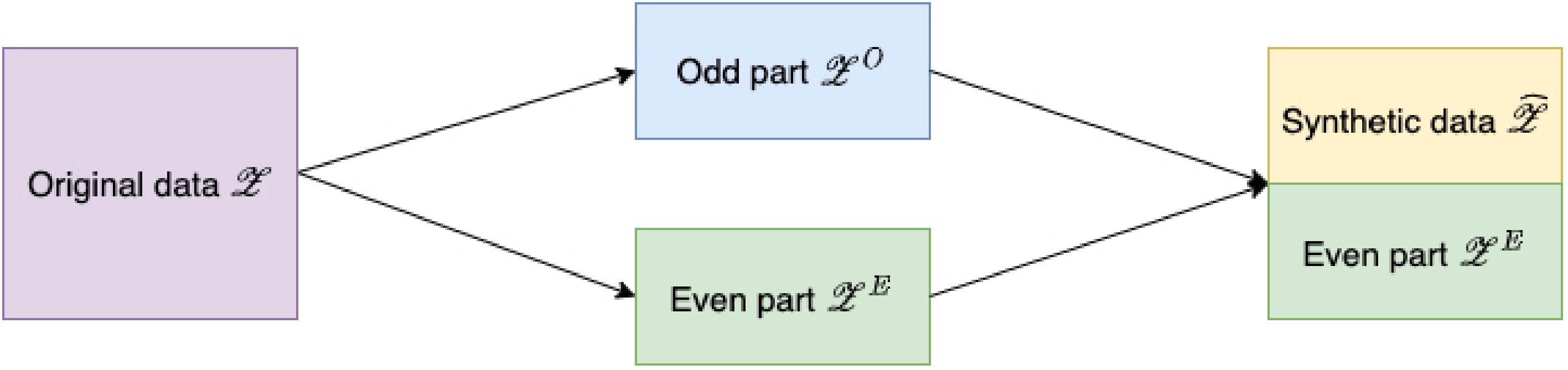
Figure 1.
Flow chart of SD filter.
The synthetic data framework clearly departs from the aforementioned error rate control procedures. Unlike conventional methods that quantify the distribution of the test statistic, the Gaussian multiplier bootstrap is employed [31,32] to construct a mirror statistic for FDR control. This framework is highly general, easily extendable to various model settings, and applicable to any scenario requiring data splitting for simultaneous hypothesis formulation and testing. By integrating the synthetic random sample with the second dataset in the testing phase, the original sample size is maintained, thereby boosting statistical power.
-
Suppose that a sequence of independent data have been observed,
$ \mathcal{Z} = \{ \mathbf{z}_1, \ldots, \mathbf{z}_{2n}\} $ $ \begin{array}{l} \mathbf{z}_i \sim F(\cdot | \boldsymbol{\beta}_k), \tau_k \lt i \leqslant \tau_{k+1}, k = 1,\ldots, K_n; i = 1, \ldots, 2n \end{array} $ (1) where, Kn is the number of change-points which could diverge with sample size
$ n $ $ \tau_{k}'s $ $ \tau_0 = 0 $ $ \tau_{K_n+1} =2n $ $ F(\cdot | \boldsymbol{\beta}_k) $ $ \boldsymbol{\beta}_k $ $ \boldsymbol{\beta}_{k} \ne \boldsymbol{\beta}_{k+1} $ The objective of this study is to detect the active set
$ \mathcal{S} = \{\tau_k, k = 1, \ldots, K_n\} $ $ \hat{\mathcal{S}} = \{ \hat{\tau}_k, k =1,\ldots, \hat{K}_n\} $ Definition 2.1 (False discovery). The candidate change-point
$ \hat{\tau}_{k} \in \hat{\mathcal{S}} $ $ \begin{array}{l}G_k:=\left[\lceil(\hat{\tau}_{k-1}+\hat{\tau}_k)/2\rceil,\lceil(\hat{\tau}_k+\hat{\tau}_{k+1})/2\rceil\right)\end{array} $ (2) where,
$ \hat{\tau}_0 = 0 $ $ \hat{\tau}_{ \hat{K}_n} = 2n $ Further, let the set
$ \mathcal{I}_0 $ $ \mathcal{I}_1 = \hat{\mathcal{S}}\cap \mathcal{I}_0^c $ $ \hat{\mathcal{S}} $ $ \mathcal{I}_1 $ $ \mathcal{I}_0 $ $ \text{FDR}(\mathcal{T})=\text{E}\left[\dfrac{|\mathcal{T}\cap\mathcal{I}_0|}{|\mathcal{T}|}\right] $ (3) where
$ \mathcal{T} $ $ \hat{\mathcal{S}} $ Synthetic data generating process
-
This subsection first introduces a synthetic data generating procedure. Following the order-preserving splitting procedure in Zou et al.[33], the data
$ \mathcal{Z} $ $ \mathcal{Z}^{O} := \{ \mathbf{z}_{2i-1}, i = 1, \ldots, n\} \text{ and } \mathcal{Z}^{E} := \{ \mathbf{z}_{2i}, i = 1, \ldots, n\} $ On the subset
$ \mathcal{Z}^{O} $ $ \hat{\mathcal{S}} = \{ \hat{\tau}_1, \ldots, \hat{\tau}_{ \hat{K}_n}\} $ $ \hat{\mathcal{S}} $ $ \mathcal{S} $ $ \hat{\mathcal{S}} $ $ \mathcal{Z}^O $ $ \mathcal{Z}^E $ $ \mathcal{Z}_{G_k}^O := \{ \mathbf{z}_{2i-1}: i \in G_k\} $ $ \mathcal{Z}_{G_k}^E := \{ \mathbf{z}_{2i}: i \in G_k\} $ $ \mathcal{Z}^{O} $ Let
$ \ell(\boldsymbol{\beta}; \mathbf{z}_i) $ $ \mathbf{z}_i $ $ \mathbf{s}_{ \boldsymbol{\beta}}(\mathbf{z}_i) = {\partial \ell(\boldsymbol{\beta}; \mathbf{z}_i)}/{\partial \boldsymbol{\beta}} $ $ \boldsymbol{\gamma} $ $ \text*{E}\{ \mathbf{s}_{\gamma}(\mathbf{z}_i)\} \ne \text*{E}\{ \mathbf{s}_{ \boldsymbol{\gamma}}(\mathbf{z}_{i^\prime})\} $ $ i $ $ i^\prime $ $ \begin{array}{l} \mathbf{s}_{ \boldsymbol{\gamma}}( \mathbf{z}_i) = \boldsymbol{\mu}_i + \boldsymbol{\zeta}_i, i =1,\ldots, 2n. \end{array} $ (4) where,
$ \boldsymbol{\mu}_i = \text*{E}[\mathbf{s}_{ \boldsymbol{\gamma}}(\mathbf{z}_i)] $ $ \mathbf{z}_i $ $ \boldsymbol{\zeta}_i = \mathbf{s}_{ \boldsymbol{\gamma}}(\mathbf{z}_i) - \text*{E}[\mathbf{s}_{ \boldsymbol{\gamma}}(\mathbf{z}_i)] $ $ \text*{Cov}(\boldsymbol{\zeta}_i) = \boldsymbol{\Sigma}^{(k)} $ $ i $ $ \tau_{k}+1 \leqslant i \leqslant \tau_{k+1} $ $ \boldsymbol{\gamma} $ $ \boldsymbol{\gamma} := \arg\min_{ \boldsymbol{\beta}} \sum_{ \mathbf{z}_i \in \mathcal{Z}^{O}} \ell(\boldsymbol{\beta}; \mathbf{z}_i) $ $ \boldsymbol{\gamma} $ $ \mathbf{s}_{ \boldsymbol{\gamma}}(\mathbf{z}_i) $ $ \mathbf{s}_i $ To monitor the change magnitude in the dataset
$ \mathcal{Z}_{G_k}^E $ $ \mathbf{s}_i^E $ $ \mathcal{Z}_{G_k}^E $ $ \begin{array}{l} \mathbf{c}_{k}(s)=\sqrt{\dfrac{s(n_k-s)}{n_k}}\left(\dfrac{1}{s} \displaystyle\sum\limits_{i \leqslant s, i \in G_k} \mathbf{s}^E_{i}-\dfrac{1}{n_k-s} \displaystyle\sum\limits_{i \gt s, i \in G_k} \mathbf{s}^E_{i}\right), \end{array} $ (5) where,
$ n_k = |G_k| $ $ s $ $ G_k $ $ \mathbf{s}^E_i $ $ \boldsymbol{\mu}_i^E + \boldsymbol{\zeta}_i^E $ $ \begin{array}{l} \mathbf{c}_{k}(s)=\sqrt{\dfrac{s(n_k-s)}{n_k}}\left(\dfrac{1}{s} \displaystyle\sum\limits_{i \leqslant s, i \in G_k} \boldsymbol{\zeta}^E_{i}-\dfrac{1}{n_k-s} \displaystyle\sum\limits_{i \gt s, i \in G_k} \boldsymbol{\zeta}^E_{i}\right) + \Delta_k(s), \end{array} $ (6) where,
$ \Delta_k(s) = \sqrt{{s(n_k-s)}/{n_k}}\left({s^{-1}} \sum_{i \leqslant s, i \in G_k} \boldsymbol{\mu}_{i}^E-(n_k-s)^{-1} \sum_{i \gt s, i \in G_k} \boldsymbol{\mu}_{i}^E\right). $ $ \hat{\tau}_k $ $ \Delta_k(s) = 0 $ $ \mathbf{c}_k $ $ \begin{array}{l} \mathbf{c}_{k}(s)=\sqrt{\dfrac{s(n_k-s)}{n_k}}\left(\dfrac{1}{s} \displaystyle\sum\limits_{i \leqslant s, i \in G_k} \boldsymbol{\zeta}^E_{i}-\dfrac{1}{n_k-s} \displaystyle\sum\limits_{i \gt s, i \in G_k} \boldsymbol{\zeta}^E_{i}\right), \text{ if } \hat{\tau}_k \in \mathcal{I}_0. \end{array} $ (7) Observing that for a certain false discovery
$ \hat{\tau}_k $ $ \mathbf{c}_{k}(s) $ $ s^{-1} \sum_{i \leqslant s, i \in G_k} \boldsymbol{\zeta}^E_{i} $ $ {(n_k - s)^{-1}}\sum_{i \gt s, i \in G_k} \boldsymbol{\zeta}^E_{i} $ $ s^{-1/2} \sum_{i \leqslant s, i \in G_k} \boldsymbol{\zeta}^E_{i} $ $ (n_k - s)^{-1/2} \sum_{i \gt s, i \in G_k} \boldsymbol{\zeta}^E_{i} $ $ \boldsymbol{\Sigma}^{(k)} $ $ n_k-s $ Based on this intuition, i.i.d random variables
$ \xi_1, \ldots, \xi_{n_k} $ $ N(0,1) $ $ \mathcal{Z} $ $ \mathcal{Z}^O $ $ \bar{ \mathbf{s}}_k^{O,-}(s) = s^{-1}\sum_{i \leqslant s, i \in G_k} \mathbf{s}^O_i $ $ \bar{ \mathbf{s}}_k^{O,+}(s) = (n_k-s)^{-1} \sum_{i \gt s, i \in G_k} \mathbf{s}^O_{i} $ $ \tilde{ \mathcal{Z}}_{G_k} $ Definition 2.2. Define the synthetic data based on the training sample as :
$ \begin{array}{l} \left\{\xi_{i}\left( \mathbf{s}^O_{i}-\bar{ \mathbf{s}}_k^{O,-}(s) \right) , i \leqslant s, i \in G_k \right\} ~~{ and } ~~\left\{\xi_{i}\left( \mathbf{s}^O_{i}-\bar{ \mathbf{s}}_k^{O,+}(s) \right), i \gt s, i \in G_k \right\}. \end{array} $ (8) By using the synthetic dataset
$ \tilde{ \mathcal{Z}}_{G_k} $ $ \begin{split} \tilde{ \mathbf{c}}_{k}(s)=\;&\sqrt{\dfrac{s(n_k-s)}{n_k}}\Bigg(\dfrac{1}{s} \displaystyle\sum\limits_{i \leqslant s, i \in G_k} \xi_{i}\left( \mathbf{s}^O_{i}-\bar{ \mathbf{s}}_k^{O,-}(s) \right)-\\& \dfrac{1}{n_k - s}\displaystyle\sum\limits_{i \gt s, i \in G_k} \xi_{i}\left( \mathbf{s}^O_{k}-\bar{ \mathbf{s}}_k^{O,+}(s) \right) \Bigg). \end{split} $ (9) Given the dataset
$ \mathcal{Z}_{G_k}^O $ $ \tilde{ \mathbf{c}}_{k}(s) $ $ \begin{split} \dfrac{1}{\sqrt{s}} \sum\limits_{i \leqslant s, i \in G_k} \xi_{i}\left( \mathbf{s}_{i}^O-\bar{ \mathbf{s}}_k^{O,-}(s) \right) \sim N\left(0, \widehat{\boldsymbol{\Sigma}}^{(k)-}\right) \\\text{ and } \dfrac{1}{\sqrt{n_k - s}}\sum\limits_{i \gt s, i \in G_k} \xi_{i}\left( \mathbf{s}_{i}^O-\bar{ \mathbf{s}}_k^{O,+}(s) \right) \sim N\left(0, \widehat{\boldsymbol{\Sigma}}^{(k)+}\right), \end{split} $ where,
$ \begin{split} \widehat{\boldsymbol{\Sigma}}^{(k)-}(s) &= \dfrac{1}{s}\displaystyle\sum\limits_{i \leqslant s, i \in G_k} \left( \mathbf{s}^O_{i}-\bar{ \mathbf{s}}_k^{O,-}(s) \right) \left( \mathbf{s}^O_{i}-\bar{ \mathbf{s}}_k^{O,-}(s) \right) ^\top \\ \widehat{\boldsymbol{\Sigma}}^{(k)+}(s) &= \dfrac{1}{n_k - s}\displaystyle\sum\limits_{i \gt s, i \in G_k} \left( \mathbf{s}^O_{i}-\bar{ \mathbf{s}}_k^{O,+}(s) \right) \left( \mathbf{s}^O_{i}-\bar{ \mathbf{s}}_k^{O,+}(s) \right)^\top \end{split} $ are two plausible estimates of
$ \boldsymbol{\Sigma}^{(k)} $ $ \tilde{\mathbf{c}}_k(s) $ $ \mathbf{c}_k(s) $ $ \mathbf{c}_k(s) $ $ \mathcal{Z}^O $ To conclude, for each candidate change point
$ \hat{\tau}_k $ $ \mathbf{c}_k(s) $ $ \tilde{ \mathbf{c}}_{k}(s) $ $ \hat{\tau}_k $ 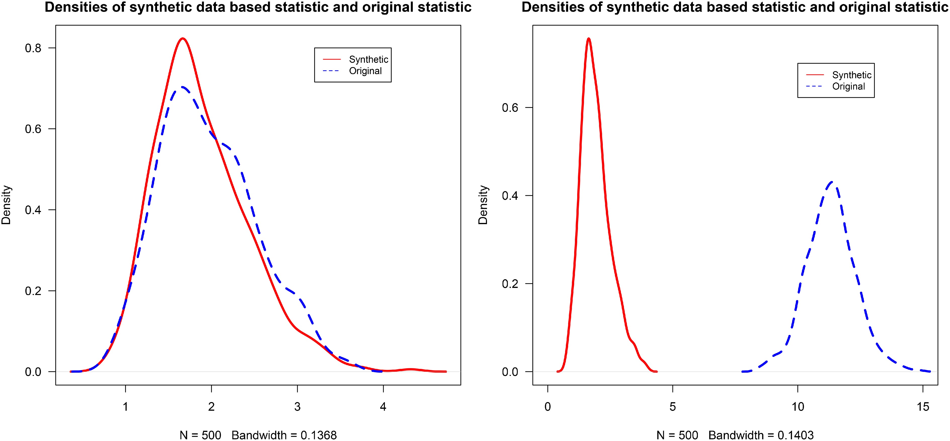
Figure 2.
Densities of the synthetic-data-based statistic and the original statistic under stationary (left) and non-stationary (right) settings. Detailed settings are described in the simulation study.
Moreover, it is worth noting that solely comparing the difference at a fixed point
$ \hat{\tau}_k $ $ \hat{\tau}_k $ $ \mathcal{Z}^O $ $ \mathcal{Z}^E $ $ \mathcal{Z}^E $ $ \ell_{q} $ $ \infty\ $ $ \mathcal{Z}^E_{G_k} $ $ \tilde{ \mathcal{Z}}_{G_k} $ $ \begin{array}{l} T_k^q = \max\limits_{ s \in G_k^*} \| \mathbf{c}_{k}(s) \|_{q} \text{ and } \tilde{T}_k^q = \max\limits_{ s \in G_k^*} \|\tilde{ \mathbf{c}}_{k}(s) \|_{q}, \text{ for } q \in \{1,2,\ldots, \infty\}. \end{array} $ (10) where, for a vector
$ \mathbf{x} \in \mathbb{R}^d $ $ \|\mathbf{x}\|_q := \big(\sum_{j=1}^d |x_j|^q\big)^{1/q} $ $ 1 \leqslant q \lt \infty $ $ \|\mathbf{x}\|_{\infty} := \max_{1 \leqslant j \leqslant d}|x_j| $ $ G_k^* $ $ G_k $ $ \underline{s} $ $ \underline{s} $ $ \widehat{\boldsymbol{\Sigma}}^{(k)-}(s) $ $ \widehat{\boldsymbol{\Sigma}}^{(k)+}(s) $ $ \boldsymbol{\Sigma}^{(k)} $ $ \hat{\tau}_k $ $ \tilde{T}_k^q $ $ T_k^q $ However, if the candidate change-point
$ \hat{\tau}_k $ $ \hat{\tau}_k \in \mathcal{I}_1 $ $ \Delta_k(s) $ $ \mathbf{c}_{k}(s) $ $ \begin{array}{l} \mathbf{r}_{k}(s)=\sqrt{\dfrac{s(n_k-s)}{n_k}}\left(\dfrac{1}{s} \sum\limits_{i \leqslant s, i \in G_k} \boldsymbol{\zeta}^E_{i}-\dfrac{1}{n_k-s} \sum\limits_{i \gt s, i \in G_k} \boldsymbol{\zeta}^E_{i}\right) \end{array} $ then in this case,
$ \begin{array}{l} T_k^q = \max\limits_{s \in G_k^*} \| \mathbf{c}_k(s)\|_q \geqslant \max\limits_{s \in G_k^*} \| \Delta_{k}(s)\|_q -\max\limits_{s \in G_k^*}\|\mathbf{r}_{k}(s) \|_q \end{array} $ where
$ \mathbf{r}_{k}(s), s \in G_k^* $ $ \tilde{ \mathcal{Z}}_{G_k} $ $ T_k^q $ $ \tilde{T}_k^q $ $ \begin{array}{l} T_k^q - \tilde{T}_k^q \geqslant \max\limits_{s \in G_k^*} \| \Delta_{k}(s)\|_q -\max\limits_{s \in G_k^*}\| \mathbf{c}_k(s) \|_q - \max_{s \in G_k^*}\| \tilde{\mathbf{c}}_k(s) \|_q \gg 0 \end{array} $ provided that the change magnitudes within
$ G_k $ FDR control via SD filter
-
Since the synthetic data in Eq. (8) mimic the distributional behavior under the null, the distributions of
$ T_k^{q} $ $ \tilde{T}_k^{q} $ $ \hat{\tau}_k \in \mathcal{I}_0 $ $ \hat{\tau}_k $ $ \begin{array}{l} W_k^q = T_k^q- \tilde{T}_k^q, \text{ for } q \in \{1, 2, \ldots, \infty\} \end{array} $ (11) discussed previously.
Moreover, the odd dataset
$ \mathcal{Z}^O $ $ \hat{\tau}_k $ $ \mathcal{Z}_{G_k}^O $ $ T_k^q(\mathcal{Z}_{G_k}^O) $ $ \hat{\mathcal{S}} $ $ \mathcal{S} $ $ T_k^q(\mathcal{Z}_{G_k}^O) \gt T_{k^\prime}^q(\mathcal{Z}_{G_{k^\prime}}^O) $ $ \hat{\tau}_k \in \mathcal{I}_1 $ $ \hat{\tau}_{k^\prime} \in \mathcal{I}_0 $ $ W_k^{side,q} $ $ \begin{array}{l} W_k^{side,q} = (T_k^q- \tilde{T}_k^q) T_k^q( \mathcal{Z}_{G_k}^O), \end{array} $ (12) After incorporating the odd dataset
$ \mathcal{Z}^O $ $ W_k^{side,q} $ $ \hat{\tau}_k \in \mathcal{I}_1 $ $ \hat{\tau}_{k^\prime} \in \mathcal{I}_0 $ $ \begin{array}{l} \dfrac{W_k^{side,q}}{W_{k^\prime}^{side,q}} = \left(\dfrac{W_k^q}{W^q_{k^\prime}}\right) \cdot \left(\dfrac{T_k^q( \mathcal{Z}_{G_k}^O)}{T_k^q( \mathcal{Z}_{G_{k^\prime}}^O)}\right) \geqslant \dfrac{W^q_k}{W^q_{k^\prime}}, \end{array} $ (13) since the second factor is typically greater than or equal to one.
Building on the definitions of
$ W_k^q $ $ W_k^{side,q} $ $ \begin{array}{l} \mathcal{T}(t) = \{ \hat{\tau}_k \in \hat{\mathcal{S}}: W_k^q \geqslant t\} \text{ or } \mathcal{T}^{side}(t) = \{ \hat{\tau}_k \in \hat{\mathcal{S}}: W_k^{side,q} \geqslant t\} \end{array} $ (14) where,
$ \mathcal{T}(t) $ $ W_k^q $ $ W_k^{side,q} $ $ \hat{\tau}_k \in \mathcal{I}_0 $ $ \begin{array}{l} \#\{ \hat{\tau}_k \in \mathcal{I}_0: W_k^{side,q} \geqslant t\} \approx \#\{ \hat{\tau}_k \in \mathcal{I}_0: W_k^{side,q} \leqslant -t\} \leqslant \#\{ \hat{\tau}_k: W_k^{side,q} \leqslant -t\} \end{array} $ (15) where,
$ W_k^{side,q} $ $ W_k^q $ $ \begin{array}{l} \text{FDR}(t) \approx \dfrac{| \mathcal{T}(t)\cap \mathcal{I}_0|}{| \mathcal{T}(t)|} \leqslant \dfrac{ \#\{k: W_k \leqslant -t\}}{ \#\{k: W_k \geqslant t\}} \end{array} $ To control the FDR at a target level
$ \alpha $ $ T(\alpha) $ $ \begin{array}{l} T(\alpha) = \min_{t} \left\{t \in \mathcal{W}: \dfrac{1+ \#\{k : W_k \leqslant -t\}}{\#\{k : W_k \geqslant t\} \vee 1} \leqslant \alpha\right\} \end{array} $ (16) where,
$ \mathcal{W} = \{ W_1, \ldots W_{ \hat{K}_n}\} \backslash \{0\} $ $ T(\alpha) $ In summary, compared with pure data-splitting methods such as MOPS and M-MOPS, the core methodological distinction of this approach lies in how the test statistics are constructed. Instead of performing inference on only half of the data, the method used generates a synthetic dataset via a Gaussian multiplier bootstrap, which integrates information from both the odd part and the reserved even part. This design increases the effective sample size and thus improves statistical power. Moreover, although the construction of
$ W_{k}^{q} $ -
The error rate control results rely on the symmetry property of the comparison statistics
$ W_k^q $ $ W_k^{side,q} $ $ \hat{\tau}_k $ Condition 3.1 (Moments and tails). Let
$ \underline{b}, \overline{b} $ $ \boldsymbol{\vartheta} \in \mathbb{S}^d $ $ \ell = 1, 2 $ $ i = 1, \ldots, 2n $ $ j = 1, \ldots, d $ $ \text*{E}[(\boldsymbol{\vartheta}^\top \boldsymbol{\zeta}_{i})^2] \geqslant \underline{b} $ $ \text*{E}[(\boldsymbol{\vartheta}^\top \boldsymbol{\zeta}_{i})^{\ell+2}] \leqslant \overline{b}^{\ell} $ $ \| \boldsymbol{\vartheta}^\top \boldsymbol{\zeta}_{i}\|_{\psi_1} \leqslant \overline{b} $ $ \beta \in [1, \infty) $ $ \| \cdot \|_{\psi_\beta} $ Condition 3.2 (Detection ability). Assume
$ \hat{K}_n \geqslant K_n $ $ \hat{\tau}_{j_1} \lt \ldots \lt \hat{\tau}_{j_{K_n}} $ $ \mathcal{T} $ $ \max_{1 \lt k \lt K_n} | \hat{\tau}_{j_k} - \tau_k| \leqslant \delta_n $ $ n \to \infty $ $ \delta_n $ Condition 3.3 (Minimum distance). Assume that
$ \mathcal{T} \subseteq \mathcal{T}(\omega_n) = \{ \mathcal{T}: \min_{j}(\tau_{j+1} - \tau_j) \geqslant \underline{\lambda}_n\} $ $ \underline{\lambda}_n $ $ \underline{\lambda}_n \geqslant n^{\eta} $ $ 0<\eta \lt 1 $ $ \underline{\lambda}_n \geqslant 2\delta_n $ A sufficient condition for Condition 3.1 (1) is that the minimum eigenvalue of
$ \boldsymbol{\Sigma}^{(k)} $ $ k = 1, \ldots, K_n $ $ d $ $ \boldsymbol{\zeta}_i $ $ \| \boldsymbol{\vartheta}^\top \boldsymbol{\zeta}_i\|_{\psi_1} \leqslant \sum_{j =1}^d \|\vartheta_j \zeta_{ij}\|_{\psi_1} \leqslant \sum_{j =1}^d \| \zeta_{ij} \|_{\psi_1} $ $ \sum_{j =1}^d \| \zeta_{ij} \|_{\psi_1} \leqslant \bar{b} $ $ \hat{\mathcal{S}} $ Let
$ \overline{n} = \max_{k = 1,\ldots, K_n} n_k $ $ \underline{n} = \min_{k = 1,\ldots, K_n} n_k $ Lemma 3.1. Assume Condition 3.1, 3.2 and 3.3 holds, then
$ \begin{array}{l}\text{Pr}\left\{\max\limits_{k\in\mathcal{I}_0}\rho(T_k^q,\tilde{T}_k^q)\leqslant c\left(\dfrac{\log^7(\overline{n})}{\underline{s}}\right)^{1/6}\mid\mathcal{Z}^O\right\}\geqslant1-C/(\underline{n})^{\kappa}\end{array} $ (17) where,
$ \rho(T_1, T_2) = \sup_{t \in (0, \infty)} | \text{Pr}(T_1 \leqslant t) - \text{Pr}(T_2 \leqslant t) | $ $ T_1 $ $ T_2 $ $ \underline{s} $ $ \min_{k = 1,\ldots, K_n} \tau_{k+1} - \tau_{k} $ $ \kappa $ $ C $ $ c $ Lemma 3.1 demonstrates that the distribution of
$ T_k^q $ Theorem 3.1. Under Condition 3.1, 3.2 and 3.3, and
$ \log^7(\hat{K}_n \bar{n})/\underline{s} \to 0 $ $ \limsup\limits_{n \to \infty} \text*{E} \left[ \dfrac{ | \mathcal{T} \cap \mathcal{I}_0|}{| \mathcal{T}|} \Big | \mathcal{Z}^O \right] \leqslant \alpha, $ for any
$ \alpha \in (0,1) $ Theorem 3.1 establishes the asymptotic FDR control property of the SD filter. The condition
$ \log^7(\hat{K}_n \bar{n} d^2)/\underline{s} \to 0 $ $ \underline{s} $ $ \delta_n/\underline{\lambda_n} \to 0 $ The FDR control for the general
$ \ell_q $ $ q = \infty $ Theorem 3.2 (FDR control for high-dimensional MCP). When
$ d \to \infty $ $ \log^7(\hat{K}_n \bar{n} d^2)/\underline{s} \to 0 $ $ q = \infty $ $ \limsup\limits_{n \to \infty} \text*{E} \left[ \dfrac{ | \mathcal{T} \cap \mathcal{I}_0|}{| \mathcal{T}|} \Big | \mathcal{Z}^O \right] \leqslant \alpha $ for any
$ \alpha \in (0,1) $ Power analysis
-
Next, the power of the SD filter is analyzed under the following signal condition.
Condition 3.4 (Minimum signal). Let
$ \boldsymbol{\delta}_{k} = \boldsymbol{\mu}_{k+1} - \boldsymbol{\mu}_k $ $ \min\limits_{k \in \mathcal{I}_1}\| \boldsymbol{\delta}^{(k)}\|_{q} \gg C\bar{\sigma}^2\sqrt{\dfrac{\log(\alpha_n \hat{K}_n\bar{n}d) }{t_k(1-t_k) \underline{n}}} $ where,
$ t_k = \tau_k/n_k $ $ \alpha_n $ $ C $ Condition 3.4 imposes a minimum signal separation between any two true change-points, ensuring their asymptotic identifiability. Similar conditions can be found in Harchaoui & Lévy-Leduc[5], Fryzlewicz[6], and Yu & Chen[13].
Theorem 3.3. Under Condtion 3.1, 3.2, 3.3 and 3.4 and
$ \log^7(\hat{K}_n \bar{n})/\underline{s} \to 0 $ $ \lim\limits_{n \to \infty} \text*{E}\left[\dfrac{| \mathcal{T} \cap \mathcal{I}_1|}{| \mathcal{I}_1|} \Big| \mathcal{Z}^O\right] = 1 $ Theorem 3.3 states that the power of SD filter approaches 1 asymptotically. Furthermore, the selection consistency property can be established.
Corollary 3.1. Under Conditions in Theorem 3.3, there is
$ \lim\limits_{n\to\infty}\text{Pr}\left\{\mathcal{S}=\mathcal{T}\mid\mathcal{Z}^O\right\}=1 $ Compared with the condition for selection consistency in Chen et al.[30], which requires
$ \min_{k \in \mathcal{I}_1}\| \boldsymbol{\delta}^{(k)}\|_2 \gg \sqrt{\log n/\underline{\lambda}_n} $ $ \underline{\lambda}_n \approx \underline{n} $ -
In this section, aseries of change-point detection experiments is conducted to evaluate the empirical performance of the SD filter. Before presenting the results, the competing methods, the Mirror with Order-Preserved Splitting (MOPS) method and its variant, the Modified-MOPS (M-MOPS) are briefly summarized, both introduced in Chen et al.[30].
The M-MOPS method controls the FDR via a mirror statistic
$ \begin{array}{l}W_k^{\text{M-MOPS}}=\dfrac{n_kn_{k+1}}{n_k+n_{k+1}}\left(\overline{\mathbf{S}}_k^{O,-}-\overline{\mathbf{S}}_k^{O,+}\right)^{\top}\Omega_n\left(\overline{\mathbf{S}}_k^{E,-}-\overline{\mathbf{S}}_k^{E,+}\right),\quad k=1,\ldots,\hat{K}_n\end{array} $ where,
$ \overline{\mathbf{S}}_k^{O,-} $ $ \overline{\mathbf{S}}_k^{O,+} $ $ \overline{\mathbf{S}}_k^{E,-} $ $ \overline{\mathbf{S}}_k^{E,+} $ $ \Omega_n $ $ \Omega_n $ $ \Omega_n = \mathbf{I}_d $ $ \begin{array}{l}W_k^{\text{MOPS}}=\dfrac{n_kn_{k+1}}{n_k+n_{k+1}}\left(\tilde{\mathbf{S}}_k^{O,-}-\tilde{\mathbf{S}}_k^{O,+}\right)^{\top}\Omega_n\left(\tilde{\mathbf{S}}_k^{E,-}-\tilde{\mathbf{S}}_k^{E,+}\right),\quad k=1,\ldots,\hat{K}_n\end{array} $ where,
$ \tilde{\mathbf{S}}_k^{O,-} $ $ \tilde{\mathbf{S}}_k^{O,+} $ $ \{ \mathbf{s}_i^O, \hat{\tau}_{k-1} \lt i \leqslant \hat{\tau}_k\} $ $ \{ \mathbf{s}_i^O, \hat{\tau}_{k} \lt i \leqslant \hat{\tau}_{k+1}\} $ $ \tilde{\mathbf{S}}_k^{E,-} $ $ \tilde{\mathbf{S}}_k^{E,+} $ Then the computational complexity of the methods is compared. Treating basic arithmetic operations as O(1), computing
$ W_{k}^{\mathrm{M}-\mathrm{MOPS}} $ $ \mathbf{c}_{k}(s) $ $ \tilde{\mathbf{c}}_{k}(s) $ $ T_{k}^{q} $ $ \tilde{T}_{k}^{q} $ $ W_{k}^{side,q} $ $ B $ Beyond computational considerations, an important issue is statistical reliability. In particular, MOPS may fail to control the FDR when the discrepancy between the candidate and true change-point sets is large. To assess the performance of all methods, 200 simulation replications were conducted and each method was evaluated using the empirical FDR and power:
$ \widehat{\text { FDR }}=\dfrac{1}{200} \sum\limits_{i=1}^{200} \dfrac{\left| \mathcal{T}_i\cap \mathcal{I}_0\right|}{| \mathcal{T}_i|} \text { and } \widehat{\text { Power }}=\dfrac{1}{200} \sum\limits_{i=1}^{200} \dfrac{\left| \mathcal{T}_i \cap \mathcal{I}_1\right|}{|\mathcal{I}_1|} $ where,
$ \mathcal{T}_i $ $ i $ The detailed pseudocode of this approach is as the Algorithm 1.
Table 1. Synthetic data filter (SD filter) for MCP detection.
${\bf Input:}$ Observed data sequence $\mathcal Z = \{{\bf{z}}_1, \dots, {\bf{z}}_{2n}\}$, target FDR level $\alpha$, suitable candidate change-point detection algorithm $\mathcal{A}(\cdot)$ ${\bf Output:}$ Selected change-point set $\mathcal T$ 1: Split data into odd and even parts:$ \mathcal{Z}^O = \{ \mathbf{z}_1, \mathbf{z}_3, \dots, \mathbf{z}_{2n-1}\}, \,\, \mathcal{Z}^E = \{ \mathbf{z}_2, \mathbf{z}_4, \dots, \mathbf{z}_{2n}\} $ 2: Detect candidate change-points $ \hat{ \mathcal{S}}=\{ \hat{\tau}_1, $ $\dots, {\hat{\tau}_{\hat{K}_n}}\}$ through $ {\mathcal{A}}({\mathcal{Z}}^O) $ 3: for $ k \in 1,\cdots,\hat{K}_n $ do 4: Define $ G_k := \left[\lceil(\hat{\tau}_{k-1}+ \hat{\tau}_k)/2\rceil, \lceil(\hat{\tau}_{k} + \hat{\tau}_{k+1})/2\rceil\right) $, where $ \hat{\tau}_0 = 0 $, $ \hat{\tau}_{ \hat{K}_n} = 2n $$ \mathcal{Z}_{G_k}^O := \{ \mathbf{z}_{2i-1}: i \in G_k\} $, $ \mathcal{Z}_{G_k}^E := \{ \mathbf{z}_{2i}: i \in G_k\} $ 5: Compute score function $ \mathbf{s}_i^E $ and $ \mathbf{c}_{k}(s)=\sqrt{\dfrac{s(n_k-s)}{n_k}}\left(\dfrac{1}{s} \sum_{i \leqslant s, i \in G_k} \mathbf{s}^E_{i}-\dfrac{1}{n_k-s} \sum_{i \gt s, i \in G_k} \mathbf{s}^E_{i}\right) $ 6: Generate synthetic data $ \tilde{ \mathcal{Z}}_{G_k} $ through $ \left\{\xi_{i}\left(\mathbf{s}^O_{i}-\bar{ \mathbf{s}}_k^{O,-}(s) \right), i \leqslant s, i \in G_k \right\} \text{ and } \left\{\xi_{i}\left(\mathbf{s}^O_{i}-\bar{ \mathbf{s}}_k^{O,+}(s) \right), i \gt s, i \in G_k \right\} $, where $ \xi_i \sim N(0,1) $ 7: Compute synthetic CUSUM $ \tilde{ \mathbf{c}}_{k}(s)=\sqrt{\dfrac{s(n_k-s)}{n_k}}\left(\dfrac{1}{s} \sum_{i \leqslant s, i \in G_k} \xi_{i}\left(\mathbf{s}^O_{i}-\bar{ \mathbf{s}}_k^{O,-}(s) \right)- \dfrac{1}{n_k - s}\sum_{i \gt s, i \in G_k} \xi_{i}\left(\mathbf{s}^O_{k}-\bar{ \mathbf{s}}_k^{O,+}(s) \right) \right) $ 8: Calculate:$ T_k^q = \max_{s \in G_k^*} \| \mathbf{c}_k(s)\|_q, \,\, \tilde{T}_k^q = \max_{s \in G_k^*} \|\tilde{ \mathbf{c}}_k(s)\|_q $ and $ W_k^{side,q} = (T_k^q - \tilde{T}_k^q) \cdot T_k^q(\mathcal{Z}_{G_k}^O) $ 9: end for 10: Obtain threshold $ T(\alpha) $: $ T(\alpha) = \min \left\{ t : \dfrac{1 + \#\{k: W_k^{side,q} \leqslant -t\}}{\#\{k: W_k^{side,q} \geqslant t\} \vee 1} \leqslant \alpha \right\} $ 11: Select final change-point set:$ \mathcal{T}^{side} = \{\hat{\tau}_k \in \hat{ \mathcal{S}} : W_k^{side,q} \geqslant T(\alpha)\} $ 12: return $ \mathcal{T}^{side} $ Simulation for multiple mean changes model
-
Consider a sequence of
$ d $ $ \boldsymbol{\mu}_{i}, i = 1,\ldots, n $ $ \{\tau_k, k = 1, \ldots, K\} $ $ \boldsymbol{\mu}_i = \boldsymbol{\mu}_{\tau_k}, \,\, \text{for} \,\, \tau_{k}+1 \leqslant i \leqslant \tau_{k+1} $ The sequence is initialized with
$ \boldsymbol{\mu}_{\tau_1} = (A/2) \mathbf{1}_d $ $ \mathbf{1}_d $ $ d $ $ \boldsymbol{\mu}_{\tau_2} $ $ r $ $ \boldsymbol{\mu}_{\tau_1} $ $ \boldsymbol{\mu}_{\tau_k} $ $ \| \boldsymbol{\mu}_{\tau_k} - \boldsymbol{\mu}_{\tau_{k+1}}\|_{\infty} = A, \quad k = 1, \ldots, K $ The data points are generated as
$ \mathbf{z}_i = \boldsymbol{\mu}_i + \boldsymbol{\epsilon}_i, i = 1, \ldots, n $ $ A $ $ d = 50 $ $ n=4,000 $ $ \tau_k=200\ k,\ k=1,\ldots,19 $ $ \tau_k=400\ k,\ k=1,\ldots,9 $ $ \mathcal{T} = \{150 k+ (-1)^{\rm{B_k}} {\rm{P_k}} \mid k = 1, \ldots 26\} $ $ \text{B}_{k} $ $ \text{P}_{k} $ $ \text{Bernoulli}\ (1/2) $ $ \text{Poisson }(5) $ $ q = \infty $ $ q \geqslant 1 $ $ q $ $ q = \infty $ $ s \in [10, 30] $ $ s $ $ n_k - s $ $ r = 1 $ $ \alpha = 0.15 $ Example 1: Normal distribution
Consider the error term
$ \boldsymbol{\epsilon}_i $ $ \boldsymbol{\Sigma} = \{\rho^{|i-j|}\}_{(i,j)} $ $ A $ $ \rho $ ● Fix
$ \rho $ ● Fix A = 1.5, and let
$ \rho $ Example 2: Beyond normal distribution
Consider the error term
$ \boldsymbol{\epsilon}_i $ $ \boldsymbol{\Sigma} = \mathbf{I}_d $ ● Fix A = 2, and let df vary in {8, 9, 10, 11, 12}.
● Fix A = 3, and let df vary in {3, 4, 5, 6, 7}.
The simulation results summarized in Figs 3 and 4 demonstrate the superior performance of the SD filter across various signal strengths and dependence structures. The results indicate that both the SD filter and M-MOPS exhibit the capability to maintain control over the false discovery rate (FDR) at the predetermined level. In contrast, MOPS struggles to maintain FDR control due to the deliberate reduction in the quality of the candidate change-point set. When the candidate change positions are significantly distant from the actual change-points, MOPS fails to perform effectively. In terms of empirical power, the SD filter consistently outperforms the M-MOPS method across all settings.
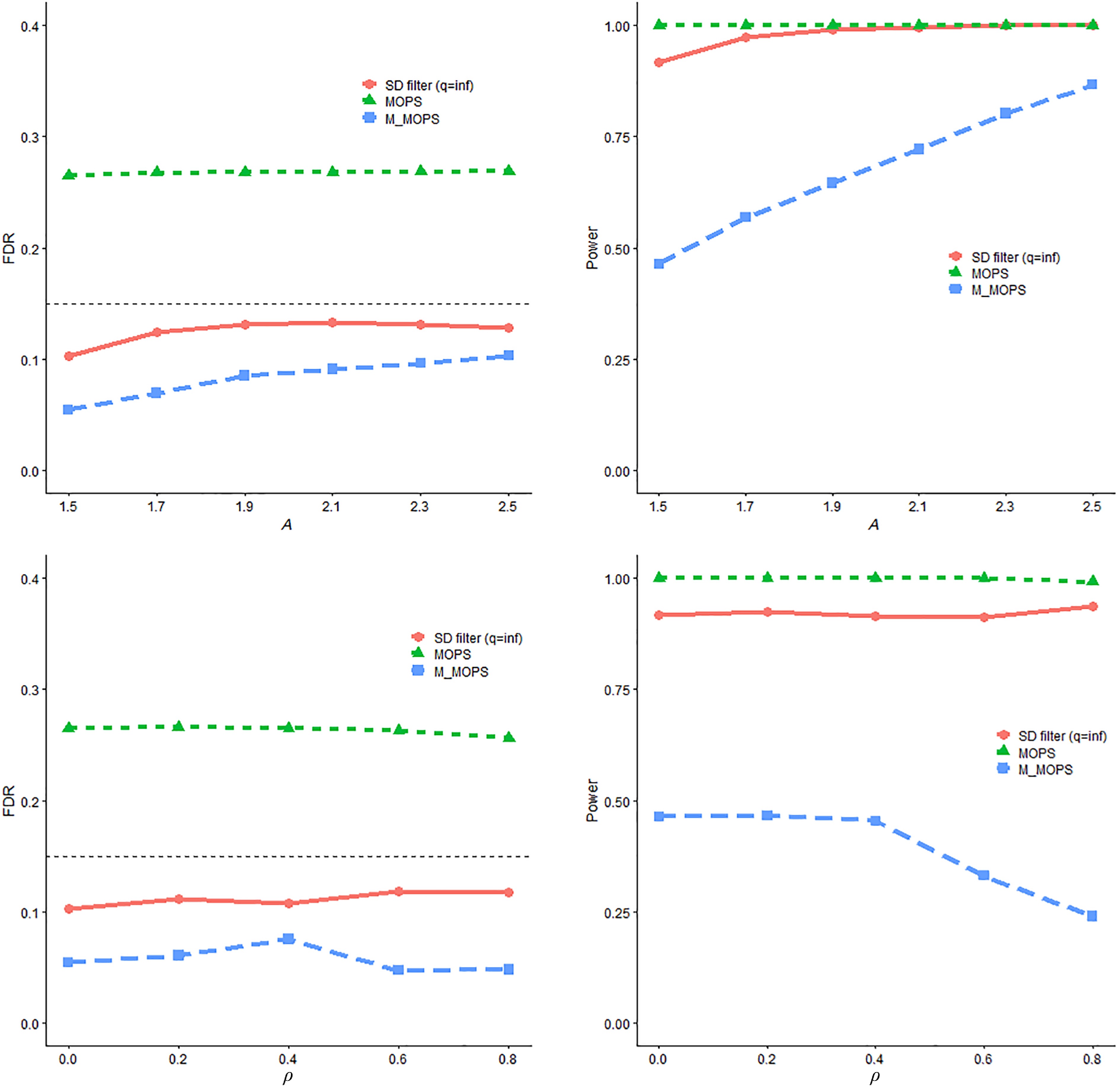
Figure 3.
FDR and power trends with respect to A and $ \rho $ for SD filter, MOPS, and M-MOPS under the mean change model, where n = 4,000, d = 50, $ \alpha $ = 0.15.
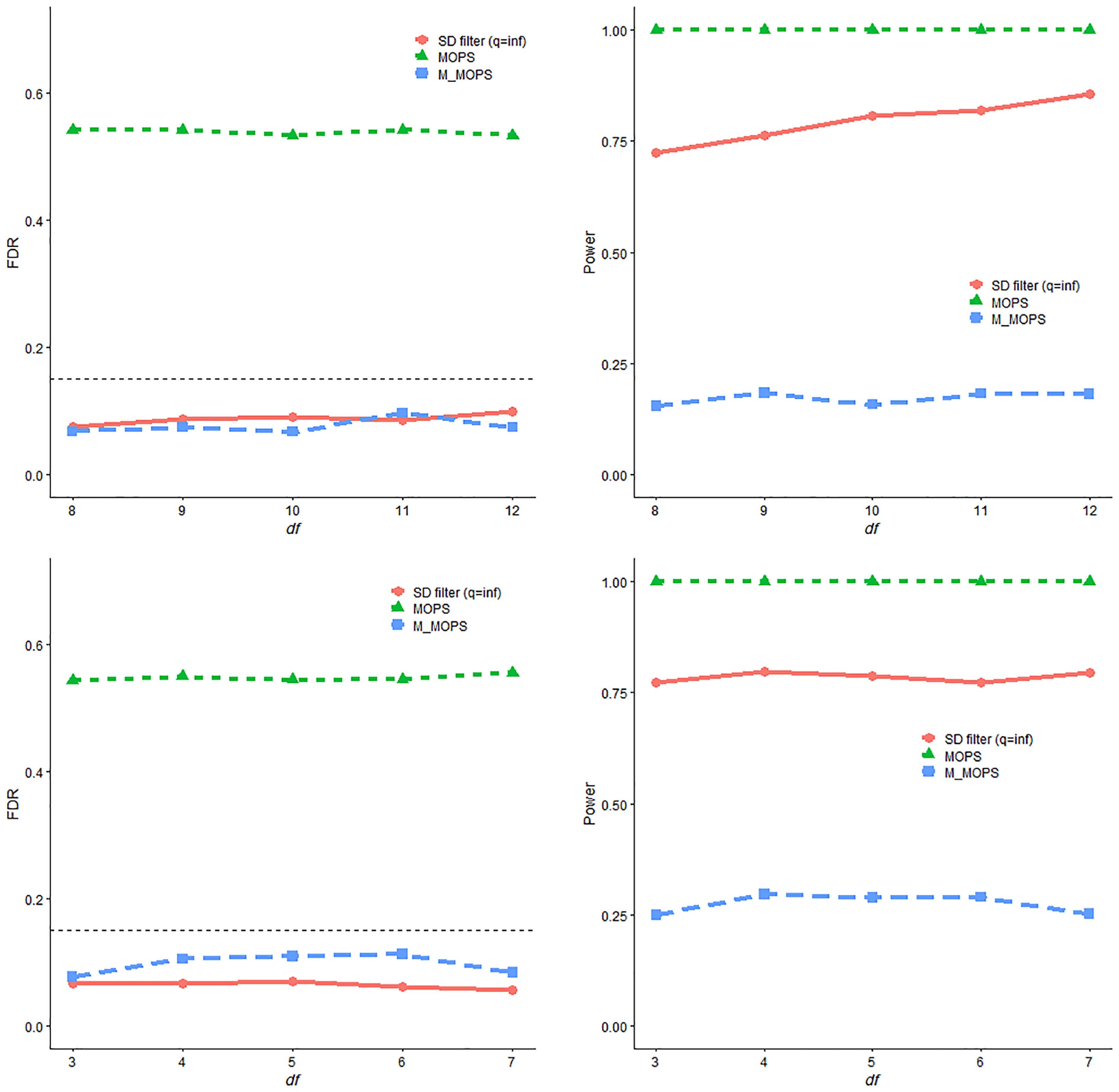
Figure 4.
FDR and power trends with respect to df of the t-distribution and chi-square distribution for SD filter, MOPS, and M-MOPS under the mean change model, where n = 4,000, d = 50, $ \alpha $ = 0.15.
Structural breaks in linear regression model
-
Consider a linear regression model with structural breaks, defined as
$ \mathbf{y}_i = \mathbf{x}_i^\top \boldsymbol{\beta}_{\tau_k} +\epsilon_i, \,\, \text{for}\,\, \tau_{k-1} \leqslant i \leqslant \hat{\tau}_k $ $ \boldsymbol{\beta}_{\tau_1} = (A/2) \mathbf{1}_d $ $ \boldsymbol{\beta}_{\tau_2} $ $ s $ $ \boldsymbol{\beta}_{\tau_1} $ $ \boldsymbol{\beta}_{\tau_k} $ $ \boldsymbol{\beta}_{\tau_{k-1}} $ $ \| \boldsymbol{\beta}_{\tau_k} - \boldsymbol{\beta}_{\tau_{k+1}}\|_{\infty} = A, \quad k = 1, \ldots, K. $ The covariates
$ \mathbf{x}_i $ $ N(\mathbf{0}_{d}, \boldsymbol{\Sigma}) $ $ \mathbf{0}_{d} $ $ \boldsymbol{\Sigma} = \{\rho^{|i-j|}\}_{(i,j)} $ $ \epsilon_i $ $ N(0,1) $ $ \mathcal{S} = \{1000 k, k = 1, \ldots, 7\} $ $ \hat{\mathcal{S}} = \{ 450 k + (-1)^{\text{B}}_{\rm k} \text{P}_{\rm k} \mid k = 1, \ldots, 16\} $ $ \text{B}_{k} \sim \text{Bernoulli}(1/2) $ $ \text{P}_k\sim\text{Poisson }(5) $ $ \alpha = 0.2 $ $ A $ $ \rho $ ● Fix
$ \rho$ ● Fix A = 0.25, and let
$ \rho $ The simulation results presented in Figs 5 and 6 display the estimated FDR and empirical power results for the linear regression model with structural breaks under various scenarios. As before, it was observed that both the SD filter and M-MOPS successfully control the FDR at the pre-specified level. Again, MOPS fails to do so due to the deliberately reduced quality of the candidate change-point set. In terms of empirical power, the SD filter still consistently outperforms M-MOPS in this setting.
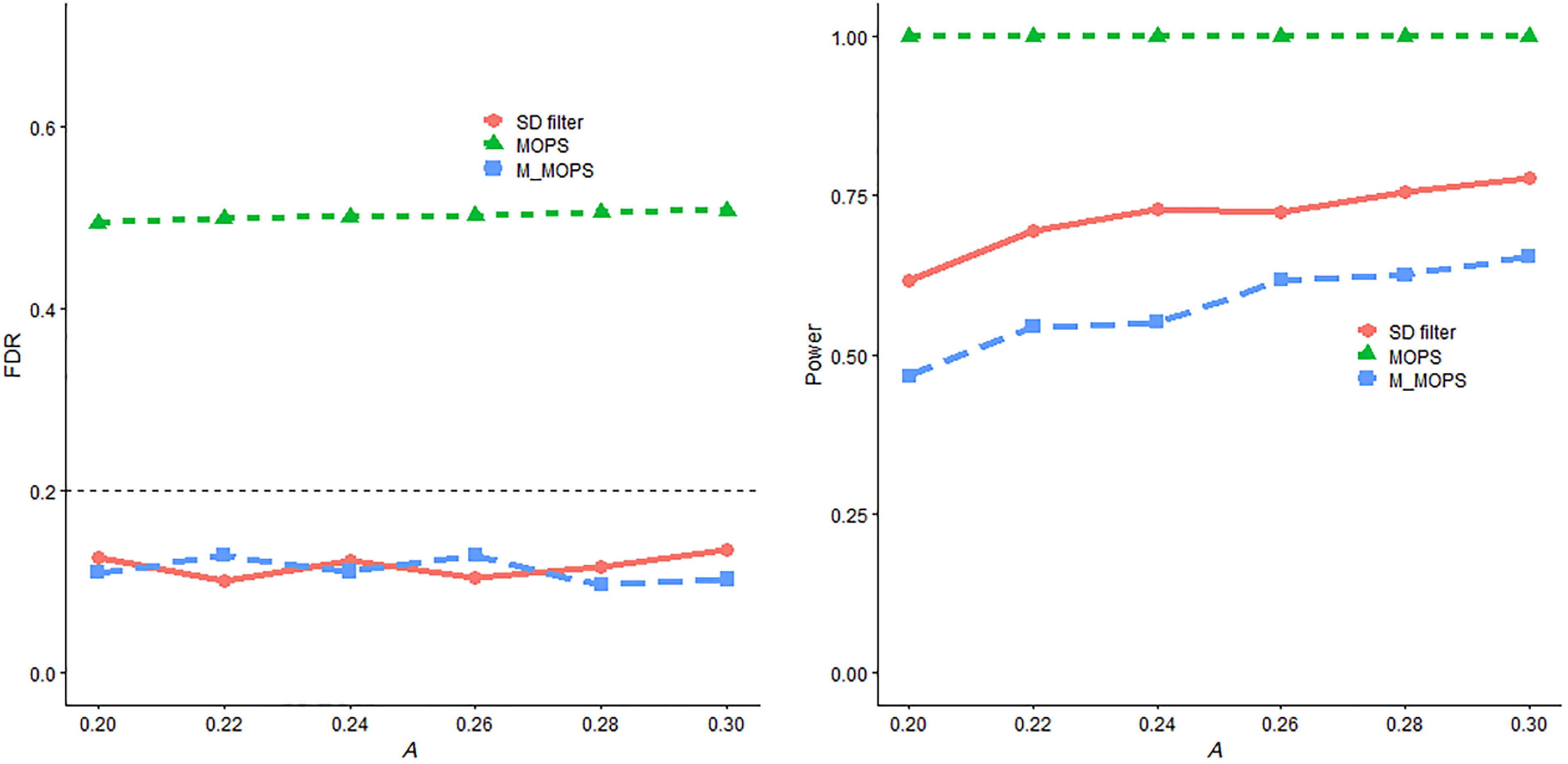
Figure 5.
FDR and power trends with respect to A for SD filter, MOPS, and M-MOPS under the structural breaks linear regression model, where n = 8,000, d = 10, $ \alpha $ = 0.2.
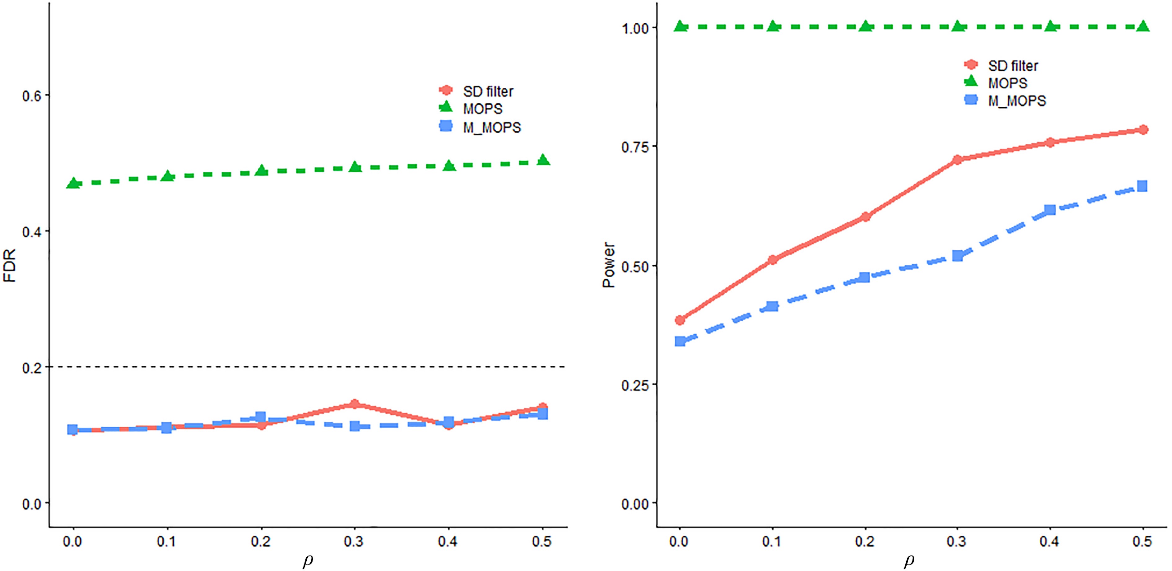
Figure 6.
FDR and power trends with respect to $ \rho $ for SD filter, MOPS and M-MOPS under the structural breaks linear regression model, where n = 8,000, d = 10, $ \alpha $ = 0.2.
-
In this section, the proposed SD filter is applied to analyze the bladder tumor micro-array dataset sourced from Bleakley & Vert[35], which is conveniently available in the ecp R package. The dataset consists of log–intensity-ratio measurements for 2,215 genetic loci obtained from 43 individuals diagnosed with bladder tumors. The primary objective is to identify change-points within the genetic loci, enabling the study to pinpoint potential influential genes related to bladder tumors. This dataset has been widely used as a benchmark in several prior studies on change-point detection[35–37], making it a representative and well-established dataset for evaluating the empirical performance of new methods. The analysis was conducted on the full dataset. However, for visualization purposes and to provide a clearer and more interpretable presentation of the results, the findings for the first ten individuals were reported, specifically individuals 3, 4, 5, 6, 7, 8, 9, 10, 14, and 15.
Firstly, the inspect method[9] is applied to narrow the scope and obtain a candidate set. To ensure optimal performance, a minimum difference of
$ 50 $ $\begin{split} \hat{\mathcal{S}} =\;& \{73,263,428,669,811,960, \\& 1050, 1378, 1436, 1559,1724, 1831, 1906, 2084\}\end{split} $ Subsequently, the SD filter, MOPS and M-MOPS are applied to further refine the results, controlling the FDR at a level of 0.1. The final sets of detected change-points from MOPS and M-MOPS are identical to
$ \hat{\mathcal{S}} $ $ \mathcal{T}_{SD} = \{73,263,428,669,811,960, 1050, 1378, 1436, 1559, 1724, 1906, 2084\} $ This result of SD filter excludes the position 1,831. Figure 7 visually demonstrates the change-points identified through the SD filter. In each plot, individual data points represent log-intensity ratios on a specific genetic locus, with each plot corresponding to a different test subject. Vertical lines are used to indicate the locations of detected change-points. The change-points identified by the SD filter are shown as dashed lines. Notably, the only solid line—positioned at 1,831—does not correspond to any apparent change across the ten individuals, highlighting the greater precision and accuracy of the SD filter in identifying true change-points.
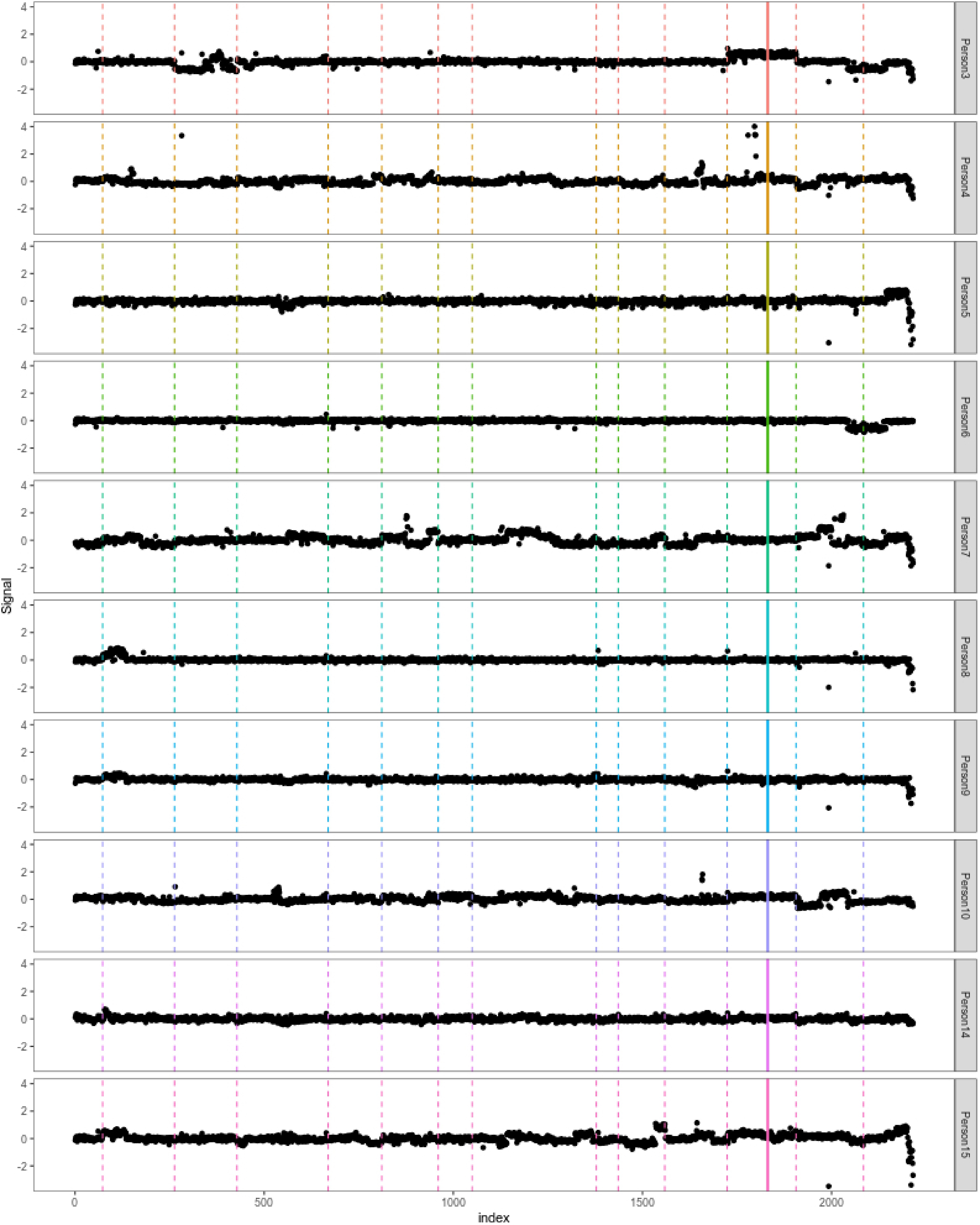
Figure 7.
Detected change-points on bladder tumor micro-array dataset (first ten persons are presented).
-
To overcome the limitations of existing FDR control methods for multiple change-point detection-particularly the drawbacks associated with data-splitting approaches, the study proposes a synthetic data filter (SD filter) for change-point detection and FDR control. After identifying potential change-points, Gaussian multiplier bootstrap is applied to generate synthetic data based on information from the detection dataset. This synthetic data is then used to construct a mirror statistic that enables control of the FDR, offering the flexibility to leverage information from the entire dataset and improve statistical power under a variety of alternatives and dimensions. The symmetry property of the mirror statistic is then established andits ability to rigorously control FDR asymptotically is proven. The detection power is also demonstrated under mild conditions. Simulation studies empirically verified the outstanding performance of the SD filter in terms of FDR control and power. The study also applies the proposed method to analyze a micro array dataset that describes the change loci of bladder tumor patients. As mentioned above, the framework of the SD filter is quite general, and it would be interesting to extend it to a broader range of cases where data splitting is required for formulating and testing hypotheses within the same dataset.
This work was supported by National Natural Science Foundation of China (Grant Nos 12271456 and 71988101), the Ministry of Education Research in the Humanities and Social Sciences (Grant No. 22YJA910002). The authors sincerely thank the editor and the referees for their constructive comments and helpful suggestions.
-
This study uses publicly available and anonymized data from the ecp R package. As the data are de-identified and distributed for open research purposes, no ethical approval was required from the authors' institution. All analyses were conducted in accordance with standard ethical guidelines for statistical research and data use.
-
The authors confirm contribution to the paper as follows: study conception and design: Sun A, Liu J; data collection: Sun A; analysis and interpretation of results: Sun A, Bi J, Liu J; draft manuscript preparation: Sun A, Bi J, Liu J. All authors reviewed the results and approved the final version of the manuscript.
-
The data that support the findings of this study are available through the ecp R package.
-
The authors declare that they have no conflict of interest.
- Copyright: © 2026 by the author(s). Published by Maximum Academic Press, Fayetteville, GA. This article is an open access article distributed under Creative Commons Attribution License (CC BY 4.0), visit https://creativecommons.org/licenses/by/4.0/.
-
About this article
Cite this article
Sun A, Bi J, Liu JY. 2026. A synthetic data approach for FDR control in change-point detection. Statistics Innovation 3: e002 doi: 10.48130/stati-0026-0002 

A synthetic data approach for FDR control in change-point detection
- Received: 22 May 2025
- Revised: 15 December 2025
- Accepted: 29 December 2025
- Published online: 28 February 2026
Abstract: In multiple change-point analysis, the resulting detection sets are typically conservative, often identifying more change points than actually exist, due to the issues of 'unreliability of assumptions' and 'unreliability of algorithms'. Therefore, controlling the false discovery rate is of vital importance to multiple change-point detection. Data-splitting-based methods have gained widespread attention for false discovery rate control. However, relying solely on a part of the dataset during the validation stage typically suffers from power loss. Instead, the study introduces a novel synthetic data framework and proposes the Synthetic Data Filter to control the false discovery rate in multiple change-point detection. Here, the study demonstrates that the proposed method effectively controls the false discovery rate and achieves asymptotic power approaching one under mild conditions. Numerical comparisons with existing methods provide evidence for the superiority of the approach in terms of both false discovery rate control and statistical power. The proposed method is further applied to a bladder tumor microarray dataset, and potential loci are identified with structural changes.