Factor-augmented group effect selection with application to gene set analysis

Variable selection is a fundamental problem in modern statistics, particularly in high-dimensional regression, where the number of predictors can greatly exceed the sample size^[1,2,3]. When covariates possess a natural grouping structure, such as sets of genetic markers belonging to the same biological pathway, the ability to select or discard groups of variables rather than individual variables becomes crucial for both interpretability and statistical efficiency. Group LASSO^[4] provides an early and influential framework for grouped selection by penalizing the $ \ell_2 $-norm of group coefficients. It has spurred a wide range of developments, including group smoothly clipped absolute deviation (group SCAD) and group minimax concave penalty (group MCP)^[5], as well as bi-level selection approaches, such as the composite MCP^[6], group bridge^[7], and group exponential LASSO^[8]. For more details on group variable selection, refer to Huang et al.^[5].

Our research is motivated by the unique data structures encountered in gene set analysis (GSA). Gene set variation analysis (GSVA)^[9] is a widely used unsupervised method that constructs, for each individual and each gene set, a Kolmogorov–Smirnov (KS) statistic comparing the distributions of expression levels for genes inside the set with those outside. The collection of such statistics along the ranked gene list yields an individualized KS curve that characterizes the enrichment profile of the gene set. Figure 1 shows examples of these curves for the Kyoto Encyclopedia of genes and genomes (KEGG)^[10] pathway "MicroRNAs in Cancer," where each curve corresponds to one individual. In practice, GSVA summarizes each curve by a single enrichment score, which is then used as the gene-set–level feature. This representation suffers from two important limitations. First, the enrichment score is marginal in the sense that it does not adjust for dependence among gene sets, and thus, the gene sets with significant enrichment scores may rise because of correlation with truly relevant ones. Second, reducing the entire curve to a single number may fail to capture the important structural features of the enrichment pattern, potentially limiting the statistical efficiency and biological interpretability^[11].

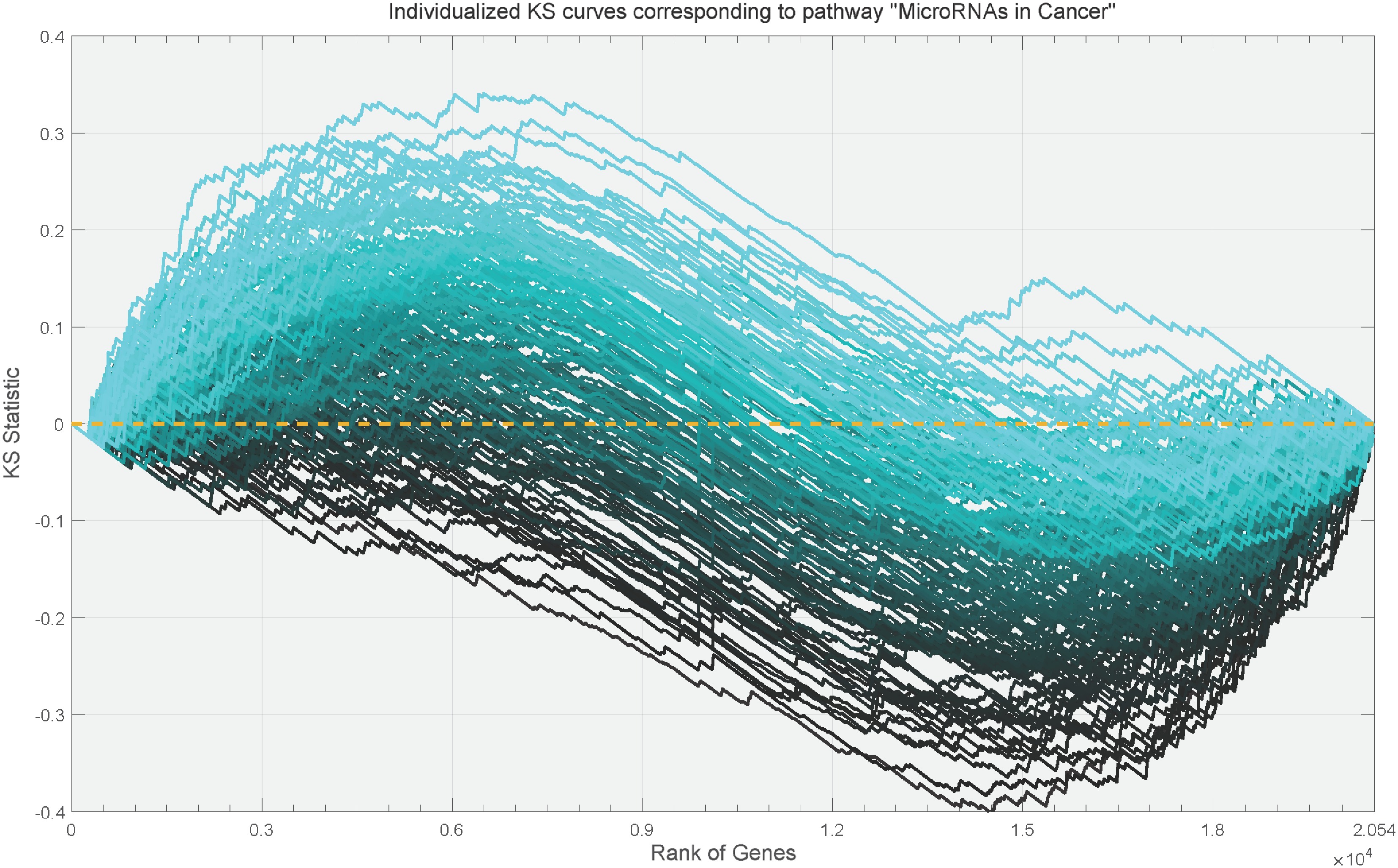
Figure 1. 

Individualized KS curves corresponding to the pathway "MicroRNAs in Cancer". Each curve corresponds to an individual and is estimated from the head and neck squamous cell carcinoma data. The depth of the curve's color is determined by the value of the extreme point in the curve.

A natural remedy is to treat the collection of genes within a set, or equivalently, the curves formed by their KS statistics, as a group, and then apply group variable selection methods to automatically identify the most important gene sets. However, the existing group variable selection methods are not well suited for this setting because gene set data typically exhibit substantially more complex structures. For instance, the design matrix of a gene set may consist of individualized curves, leading to dimensions of size n × p, where n is the sample size and p is the number of genes. When the group size is very large, conventional group selection methods are prone to computational difficulties such as non-convergence. Moreover, strong correlations among genes or functional-like curve structures within a set result in severe multicollinearity, violating the irrepresentable conditions required for consistent group selection^[12,13]. Consequently, truly important gene sets cannot be reliably recovered under standard penalized regression. A few methods, such as the elastic net^[14] and factor-adjusted regularized model selection (Farm-Select)^[15], offer partial remedies by addressing multicollinearity, but they neither exploit the grouping of covariates nor accommodate complex within-group structures.

To address the challenges of high-dimensional grouped data with complex group structures, we propose factor-augmented group effect selection (FAGES), a novel group variable selection method that simultaneously identifies important groups, provides comparable estimates of group effect sizes, and determines their effect directions. The key idea is to represent each group of variables by a low-dimensional latent factor that captures its main variation, and then specify a factor-augmented regression model accounting for the additive contributions of all groups. In particular, when the grouped variables take the form of curves (e.g., individualized KS curves in GSA), the latent factor representation can be viewed as functional principal component analysis (FPCA)^[16,17], enabling FAGES to effectively handle functional data structures. By applying a variable selection penalty, FAGES achieves both group identification and effect estimation in a unified framework. We establish the consistency of parameter estimation and group selection under mild conditions, and numerical studies demonstrate that FAGES reliably recovers relevant groups even under model misspecification. As an illustration, we apply FAGES to head and neck squamous cell carcinoma (HNSCC) transcriptomic data and detect the biological pathways that play key roles in disease development.

For a vector a = (a_j)_{p × 1}, let ||a||_q = ($\sum_{j=1}^p $|a_j|^q)^1/q with q $ \in $ [0, ∞]. For a symmetric matrix A = (A_ij)_{p × p}, σ_j(A) denotes the $ j $-th largest eigenvalue of matrix A, $ ||{\bf{A}}\|_F^2=\sum_{i}\sum_{j}A_{ij}^2 $, and ||A||_q = max{||Aa||_q, ||a||_q = 1}. Besides, a_n $ \asymp $ b_n if there are positive constants c and C such that c ≤ a_n/b_n ≤ C. Notations {a_j}, and {A_j} represent a set of vectors {a₁, …, a_p} and a set of matrices {A₁, …, A_p}, respectively. In addition, notation diag(a) denotes the diagonalizing operator of vector a and diag(A₁, …, A_p) denotes the block-diagonalizing operator of a series of matrices {A_j}. Moreover, we define σ_max(A) = σ₁(A) and σ_min(A) = σ_p(A) as the largest and smallest eigenvalues of a symmetric matrix A $ \in\mathbb{R}^{p\times p} $, respectively.

Background

Approximate factor model

A multivariate variable X_i = (X_i1, …, X_ip)^T is termed to follow a factor model if

where, X = (X₁, …, X_n)^T is the sample matrix of X_i, F= (F₁, …, F_n)^T is the matrix of latent factor F_i = (f_i1, …, f_iK)^T, $ {\boldsymbol{\Lambda}} $ = (λ₁, …, λp)^T is the loadings matrix with λ_j = (λ_j1, …, λ_jK)^T, and e = (e₁, …, e_n)^T is the matrix of the idiosyncratic component e_i = (e_i1, …, e_ip)^T. The factor model is known as approximate factor model (AFM) if the idiosyncratic components have cross-sectional correlation, which has been verified to be effective in explaining the correlation structure of variables in econometrics^[18].

Principal components analysis (PCA) and AFM are closely related^[18]. Specifically, F and $ {\boldsymbol{\Lambda}} $ can be estimated by the following restricted minimization:

The minimizers of the above restricted minimization are explicit and unique. Suppose the singular value decomposition X = $ \sum_{s=1}^p $d_sU_sV_s^T , where U_s is the s-th left singular vector, V_s is the s-th right singular vector, and d_s is the s-th singular value of X. Then $ \hat{{\bf{F}}}=\sqrt n({\boldsymbol{U}}_1,\cdots,{\boldsymbol{U_K}}) $ and $ \hat{\Lambda}={\bf{X}}^\top \hat{{\bf{F}}}/\sqrt n $. That is, $ \hat{{\bf{F}}} $ consists of the first K principal components (PCs) of X.

Note that AFM is further connected to functional PCA, which is used to characterize the main pattern of the individualized trajectories around an overall mean trend function in functional data analysis^[19]. In the simulation example on functional regression, we introduce how to use AFM to handle the functional data through the projection-PCA^[16].

Group variable selection approaches

Multivariate variable X_i is termed to have a group structure if there is a series of sets $ \{{\cal{M}}_1,\cdots,{\cal{M}}_J\} $ such that X_i = $ ({\boldsymbol{X}}_{i{\cal{M}}_1}^\top,\dots,{\boldsymbol{X}}_{i{\cal{M}}_J}^\top)^\top $. Multivariate GLM with grouped variables refers to

where, $ {\boldsymbol{\mu}} $ = E(y) and y = (y₁, …, y_n)T $\in\mathbb{R}^{n} $ is the response that follows the exponential family distribution^[20]. Here, 1 $ \in\mathbb{R}^{n} $ is the all-one vector, $ {\bf{X}}_{{\cal{M}}_j}=({\boldsymbol{X}}_{1,{\cal{M}}_j},\dots,{\boldsymbol{X}}_{n,{\cal{M}}_j})^\top\in\mathbb{R}^{n\times p_j} $ is the design matrix of variables in group $ {\cal{M}}_j $, and $ {{\boldsymbol{\beta}}}_{{\cal{M}}_j}\in\mathbb{R}^{p_j} $ is the corresponding regression coefficient vector, where $ p_j=|{\cal{M}}_j| $ and $ s\in{\cal{M}}_j $. Moreover, X = $ ({\bf{1}},{\bf{X}}_{{\cal{M}}_1},\dots, {\bf{X}}_{{\cal{M}}_J})\in\mathbb{R}^{n\times(1+\sum_{j=1}^J p_j)} $ and β = $ (\beta_0,{{\boldsymbol{\beta}}}_{{\cal{M}}_1}^\top,\dots,{{\boldsymbol{\beta}}}_{{\cal{M}}_J}^\top)^\top\in\mathbb{R}^{1+\sum_{j=1}^J p_j} $; g(·) is known as the canonical link function. In addition, we assume that these sets are known in advance from preliminary information. For example, the KEGG^[10] database is designed according to the functional pathways of genes, while the gene ontology (GO)^[21] database is made based on the ontology annotations of genes.

The regression coefficient β can be estimated through the penalized likelihood^[22] shown below:

where, $ {\cal{L}}({\boldsymbol{\eta}})=-({\bf{y}}^\top{\boldsymbol{\eta}}-{\bf{1}}^\top b({\boldsymbol{\eta}})) $ is the negative log-likelihood function and b'(x) is the derivative of b(x); η is known as the linear predictor, which is equal to Xβ in this case; b(·) is a known function satisfying b'(x) = g⁻¹(x); and ρ_λ(·) is a group variable selection penalty with a penalizing parameter λ. There are two categories of group variable selection penalties: group-level selection penalty, such as group LASSO^[4], group SCAD, and group MCP^[5], and bi-level selection penalty, including composite MCP (cMCP)^[6], group bridge approach^[7], and group exponential LASSO (GEL)^[8]. For example, the group MCP is defined as:

where, a > 2 is a tuning parameter. As well, the expression of GEL is given by

where, a > 0 is an alternative tuning parameter. In addition, a weight w_β is generally applied to adjust λ as w_βλ to trade off the influence of group size. For group-level penalty, w_β is usually set as $ \sqrt{{{\rm{dim}}}({{\boldsymbol{\beta}}})} $; for bi-level penalty, w_β is often estimated as dim(β).

Note that whether ρ_λ(||β||) is called group- or bi-level penalty depends on the type of norm ||·|| rather than its expression. The penalty is called group-level penalty if it measures the $ \ell_2 $-norm of β, while it is termed bi-level penalty if it measures the $ \ell_1 $-norm of β. In addition, group-level penalty can only select the important groups, whereas bi-level penalty can select important variables and groups simultaneously. For more details, refer to Huang et al.^[5].

Statistical methodology of FAGES

Representation

FAGES is a novel group variable selection method that combines the AFM and group variable selection approach reviewed in the previous section. Suppose a multivariate variable with group structure, i.e., X_i = $(1,{\boldsymbol{X}}_{i,{\cal{M}}_1}^\top,\dots,{\boldsymbol{X}}_{i,{\cal{M}}_J}^\top)^\top $; in particular, the multiple variables $ {\boldsymbol{X}}_{i,{\cal{M}}_j} $ are usually highly correlated in the group $ {\cal{M}}_j $. FAGES assumes these multiple variables to follow an AFM:

where, $ {\bf{X}}_{{\cal{M}}_j}=({\boldsymbol{X}}_{1,{\cal{M}}_j},\dots,{\boldsymbol{X}}_{n,{\cal{M}}_j})^\top $, $ {\bf{F}}_{{\cal{M}}_j}=({\boldsymbol{F}}_{1,{\cal{M}}_j},\dots,{\boldsymbol{F}}_{n,{\cal{M}}_j})^\top $, $ {\boldsymbol{\Lambda}}_{{\cal{M}}_j}= ({\boldsymbol{\lambda}}_{1,{\cal{M}}_j},\dots,{\boldsymbol{\lambda}}_{p_j,{\cal{M}}_j}) $, and $ {\bf{e}}_{{\cal{M}}_j}=({\boldsymbol{e}}_{1,{\cal{M}}_j},\dots,{\boldsymbol{e}}_{n,{\cal{M}}_j})^\top $.

Since the major information of $ {\bf{X}}_{{\cal{M}}_j} $ is represented by $ {\bf{F}}_{{\cal{M}}_j} $, it is able to detect the important group $ {\cal{M}}_j $ by looking at the significance of the corresponding latent factor $ {\bf{F}}_{{\cal{M}}_j} $. Motivated by this principle, FAGES considers a new group-wise factor-augmented GLM (GF-GLM), which addresses the regression between a response y and the multiple latent factors of all groups:

Compared with the high-dimensional GLM (3), the grouped factor-augmented GLM discards the redundant parts $ \{e_{i{\cal{M}}_j}\} $ and reduces the dimension of the model from $ \sum_j^J $p_j to $ \sum_j^J $K_j. Compared with the factor-augmented regression^[23], the grouped factor-augmented GLM allows the latent factors of different groups to be presented in the same regression, so that it is able to correctly prioritize the groups and make the valid inferences. In addition, if only a few latent factors of groups have significant associations with phenotype, the group LASSO and its modifications can be applied to select the non-zero $ {{\boldsymbol{\theta}}}_{{\cal{M}}_j} $.

When the grouped factor-augmented GLM is misspecified, FAGES is still able to select the important groups with high precision. Specifically, consider the following model:

Here, $ \eta_i^F=\beta_0+\sum_j{\boldsymbol{F}}_{i{\cal{M}}_j}^\top{\boldsymbol{\theta}}_j $ and $ \eta_i^e=\sum_j{\boldsymbol{e}}_{i{\cal{M}}_j}^\top{\boldsymbol{\beta}}_{{\cal{M}}_j} $, which means that both the latent factors $ \{{\boldsymbol{F}}_{i{\cal{M}}_j}\} $ and the idiosyncratic component $ \{{\boldsymbol{e}}_{i{\cal{M}}_j}\} $ have effects on $ y_i $. Using the Taylor expansion, this model reduces to

indicating that the latent factors $ \{{\boldsymbol{F}}_{{\cal{M}}_j}\} $ can describe the main variation of y_i as long as they carry most information of $ \{{\boldsymbol{X}}_{{\cal{M}}_j}\} $. This is why FAGES can find the important groups and accurately estimate the group effects even if the grouped factor-augmented GLM is misspecified. In the literature, such an approximation has been utilized by Hall et al.^[24] to analyze the discrete functional data. They also found that a top few functional PCs (FPCs) can sufficiently describe the main variation of discrete functional data, offering the empirical confirmation of the robustness of our grouped factor-augmented generalized linear model (GLM) model.

In practice, we adopt a data-adaptive rule to select the number of factors. Specifically, for each group $ {\cal{M}}_j $, let {σ_jk}_k≥1 denote the squared eigenvalues of n⁻¹${\bf{X}}_{{\cal{M}}_j}^\top{\bf{X}}_{{\cal{M}}_j} $, truncated at K_max for stability. We consider three complementary criteria. The first is a gap-ratio statistic^[25]:

and we set $ K_j^{{\rm{DR}}}=\arg\max_{2\le k\le K_{\max}} z_{jk} $. The second is an eigenvalue-ratio statistic^[26]:

yielding $ K_j^{{\rm{ER}}}=\arg\max_{1\le k\le K_{\max}} r_{jk} $. The third criterion applies a hard threshold on the spectrum of the standardized group variables^[27]: letting $ \tilde \sigma_{jk} $ be the eigenvalues of the sample correlation matrix of $ {\bf{X}}_{{\cal{M}}_j} $, we define

Finally, we take the conservative aggregation

and estimate the group factors $ {\bf{F}}_{{\cal{M}}_j} $ accordingly, which empirically stabilizes inference by avoiding overestimation of K_j across heterogeneous group sizes and within-group correlation structures. We adopt this conservative strategy because Fan et al.^[27] pointed out that the primary practical risk in factor-augmented models is not understimating the number of factors but rather including too many spurious factors, where subsequent inference may be adversely affected.

Estimation and inference

In the implementation, FAGES first estimates the latent factor of each group through the PCA and then yields the related coefficient using the penalized likelihood below:

where, $ {\cal{L}}({\boldsymbol{\eta}}) $ is the negative log-likelihood function; $ {\boldsymbol{\eta}}=\hat{{\bf{F}}}{{\boldsymbol{\theta}}} $ is the linear predictor; $ \hat{{\bf{F}}}=({\bf{1}},\hat{{\bf{F}}}_{{\cal{M}}_1},\dots,\hat{{\bf{F}}}_{{\cal{M}}_J}) $, where $ \hat{{\bf{F}}}_{{\cal{M}}_j} $ is the first K_j PCs of $ {\bf{X}}_{{\cal{M}}_j} $; ||·|| may be the $ \ell_2 $- or the $ \ell_1 $-norm, with respect to group- and bi-level selection approaches; and w_j is a given weight corresponding to group $ {\cal{M}}_j $. This penalized likelihood reduces to the traditional penalized likelihood if the latent factors are observed or their consistent estimators are given. The block descent algorithm^[28] can be used to solve (Eq. [15]) in a computationally efficient manner.

After obtaining the minimizer $ \hat{{\boldsymbol{\theta}}} $, we propose to quantify the strength of group effect of $ {\cal{M}}_j $ by using the following averaged group effect estimate:

This averaged group effect estimate is based on the fact that multiple latent factors may exist within a group and their directions are not identifiable under the AFM/PCA representation, rendering individual coefficient signs uninformative. By aggregating the fitted group-specific signal across samples, the averaged group effect provides a meaningful and comparable summary of the overall group contribution regardless of factor orientation.

With the same motivation, we propose to determine the related effect direction by the sign of certain well-defined correlation statistics $ \widehat{{\rm{cor}}}(\hat{{\bf{F}}}_{{\cal{M}}_j}\hat{{\boldsymbol{\theta}}}_{{\cal{M}}_j},{\bf{y}}) $. For example, the rank correlation

has been demonstrated to be robust for modelling the dependency of two variables^[29]. Other correlations like Kendall-$ \tau $ correlation are also appropriate to define the sign of the cluster effect. Although the factors of a group $ \hat{{\bf{F}}}_{{\cal{M}}_j} $ themselves lack a straightforward statistical interpretation, their biological significance can be elucidated by examining the signs of certain marker genes in the loading matrix $ \hat{{\boldsymbol{\Lambda}}}_{{\cal{M}}_j} $. This approach facilitates a deeper understanding of the underlying biological implications of the factors. With this specification of the averaged group effect, FAGES is able to rank the importance of significant groups and judge the related effect directions toward phenotype.

Large sample property

Denote $ \hat{{\bf{F}}}_{{\cal{M}}_j} $ as the matrix consisting of the first K_j PCs of the matrix $ {\bf{X}}_{{\cal{M}}_j} $ and $ \hat{{\boldsymbol{\Lambda}}}_{{\cal{M}}_j}={\bf{X}}_{{\cal{M}}_j}^\top\hat{{\bf{F}}}_{{\cal{M}}_j}/n $, $ \hat{{\bf{V}}}_{{\cal{M}}_j} $ as the (K_j × K_j) diagonal matrix consisting of the first K_j eigenvalues of matrix $ {\bf{X}}_{{\cal{M}}_j}^\top{\bf{X}}_{{\cal{M}}_j}/(np_j) $, and $ {\bf{H}}_{{\cal{M}}_j}^\top=\hat{{\bf{V}}}_{{\cal{M}}_j}^{-1}(\hat{{\bf{F}}}_{{\cal{M}}_j}^\top{\bf{F}}_{{\cal{M}}_j}/n)({\bf{\Lambda}}^\top{\boldsymbol{\Lambda}}/p_j) $. Denote $ {\bf{H}}_{{\cal{M}}}={{\rm{diag}}}({\bf{H}}_{{\cal{M}}_1},\dots,{\bf{H}}_{{\cal{M}}_{J_0}}) $, $ {\bf{H}}_{{\cal{M}}^c}={{\rm{diag}}}({\bf{H}}_{{\cal{M}}_{J_0+1}},\dots,{\bf{H}}_{{\cal{M}}_{J}}) $, and H = $ {{\rm{diag}}}({\bf{H}}_{{\cal{M}}},{\bf{H}}_{{\cal{M}}^c}) $. Let $ {{\boldsymbol{\theta}}}^\star=(\theta_0^\star,({{\boldsymbol{\theta}}}^\star_{{\cal{M}}_1})^\top,\dots,({{\boldsymbol{\theta}}}^\star_{{\cal{M}}_q})^\top) $ be the real regression coefficient vector. Denote $ {\cal{M}}=\{{\cal{M}}_j,||{{\boldsymbol{\theta}}}_{{\cal{M}}_j}^\star||_2\neq 0\} $, $ {\cal{M}}^c=\{{\cal{M}}_j, ||{{\boldsymbol{\theta}}}_{{\cal{M}}_j}^\star||_2=0\} $, $ {{\boldsymbol{\theta}}}^\star_{{\cal{M}}}=(\theta_0^\star,({{\boldsymbol{\theta}}}^\star_{{\cal{M}}_1})^\top,\dots,({{\boldsymbol{\theta}}}^\star_{{\cal{M}}_{J_0}})^\top)^\top $, and $ {{\boldsymbol{\theta}}}^\star_{{\cal{M}}^c}=(({{\boldsymbol{\theta}}}^\star_{{\cal{M}}_{J_0+1}})^\top,\dots,({{\boldsymbol{\theta}}}^\star_{{\cal{M}}_{J}})^\top)^\top $ = 0. Next, $ {{\rm{E}}}(y_i)=\mu_i=b'({\boldsymbol{F_i^\top}}{{\boldsymbol{\theta}}}^\star) $, $ {{\rm{var}}}(y_i)=\phi_0b''(\mu_i)=\phi_0b''({\boldsymbol{F_i^\top}}{{\boldsymbol{\theta}}}^\star) $, and W₀ = ϕ₀diag$ (b''({\boldsymbol{F}}_1^\top{{\boldsymbol{\theta}}}^\star),\dots,b''({\boldsymbol{F_n^\top}}{{\boldsymbol{\theta}}}^\star)) $. We consider the standard exponential family distribution so that the dispersion parameter ϕ₀ = 1. Let $ {\boldsymbol{\epsilon}}={\bf{y}}-b'({\bf{F}}{{\boldsymbol{\theta}}}^\star) $ be the residual vector, $ {\boldsymbol{\varepsilon}}={\bf{W}}_0^{-1/2}({\bf{y}}-b'({\bf{F}}{{\boldsymbol{\theta}}}^\star)) $ be the scaled residual vector, and $ {\boldsymbol{\delta}}=(\hat{{\bf{F}}}_{{\cal{M}}}-{\bf{F}}_{{\cal{M}}}{\bf{H}}_{{\cal{M}}}){\bf{H}}_{{\cal{M}}}^{-1}\theta^\star $ be the estimation error of significant latent factors. In addition, denote $ {\bf{C}}_{{\cal{M}}_j{\cal{M}}}=\lim_{n\to\infty}{\bf{H}}^\top_{{\cal{M}}_j}{\bf{F}}^\top_{{\cal{M}}_j}{\bf{W}}_0{\bf{F}}_{{\cal{M}}}{\bf{H}}_{{\cal{M}}} /n $ and $ {\bf{C}}_{{\cal{M}}{\cal{M}}}=\lim_{n\to\infty}{\bf{H}}^\top_{{\cal{M}}}{\bf{F}}^\top_{{\cal{M}}}{\bf{W}}_0{\bf{F}}_{{\cal{M}}}{\bf{H}}_{{\cal{M}}}/n $.

The following conditions facilitate the proofs of the theorems.

(A1) For all j, the group of variables $ {\boldsymbol{X}}_{i,{\cal{M}}_j} $, the associated common factor $ {\boldsymbol{F}}_{i,{\cal{M}}_j} $, the factor loading matrix $ {\bf{\Lambda}}_{{\cal{M}}_j} $, and the idiosyncratic components $ {\boldsymbol{e}}_{i,{\cal{M}}_j} $ satisfy the standard approximate factor condition given in the supplementary materials.

(A2) The scaled residual ε = (ε₁, …, ε_n)^T is a vector of IID variables, which satisfies that for all i, E(ε_i) = 0 , var(ε_i) = 1, and E(exp(tε_i)) ≤ exp(τ₀t²/2) for all t $ \in $ R, where τ₀ is a scale parameter of the tail. Next, {ε_i}, $ \{F_{i,{\cal{M}}_j}\}_{1\leq j\leq p} $, $ \{e_{i,{\cal{M}}_j}\}_{1\leq j\leq p} $ are mutually independent groups. Furthermore, max_iE(|ε_i|³) = O(1) and $ n^{-\frac32}\sum_{i=1}^n||{\boldsymbol{F}}_{i,{\cal{M}}}^\top{\bf{H}}_{{\cal{M}}}{\bf{C}}_{{\cal{MM}}}^{-2}{\bf{H}}_{{\cal{M}}}^\top{\boldsymbol{F}}_{i,{\cal{M}}}||_2^3\to $ 0.

(A3) There is a positive constant c₀ such that −c₀ < min_iη_i ≤ max_iη_i < c₀, where $ \eta_i={\boldsymbol{F_i^\top{\boldsymbol{\theta}}^\star}} $ for all $ i\in\{1,\dots,n\} $. There is a constant $ c_1 $ such that $ |b'(\eta_i)-b'(\eta_j)|\leq c_1|\eta_i-\eta_j| $ and $ |b''(\eta_i)-b''(\eta_j)|\leq c_1|\eta_i-\eta_j| $ for all $ i,j\in\{1,\dots,n\} $. Furthermore, there is a positive constant $ \sigma_0 $ such that $ \sigma_0<\sigma_{\min }({\bf{C}}_{{\cal{M}}_j{\cal{M}}}^\top{\bf{C}}_{{\cal{M}}_j{\cal{M}}})\leq\sigma_{\max }({\bf{C}}_{{\cal{M}}_j{\cal{M}}}^\top{\bf{C}}_{{\cal{M}}_j{\cal{M}}})<\sigma_0^{-1} $ and $ \sigma_0<\sigma_{\min }({\bf{C}}_{{\cal{M}}{\cal{M}}})\leq\sigma_{\max }({\bf{C}}_{{\cal{M}}{\cal{M}}})<\sigma_0^{-1} $ for all $ j\in\{1,\dots,J\} $.

(A4) The concave penalty $ \rho_\lambda(\cdot) $ with concavity parameter $ a $ satisfies the condition that $ \rho_\lambda(||x||) $ is increasing and concave in $ ||x||\in[0,+\infty) $ with $ \rho_\lambda(0)=0 $, and that $ \rho_\lambda(||x||) $ is differentiable in $ ||x||\in(0,+\infty) $ with $ \rho_\lambda'(0):=\rho_\lambda'(0+). $ In addition, $ \rho_\lambda'(||x||)\geq a_1\lambda $ for all $ ||x||\in[0,a_2\lambda] $, and $ \rho_\lambda'(||x||)=o(n^{-1/2}) $ for all $ ||x||\in[a\lambda,+\infty) $, for any $ a>a_2 $.

(A5) The dimensions of the latent factors $ \{K_j\} $ are bounded, the dimensions of the variables of groups $ \{p_j\} $ satisfy $ p_j\asymp n $ for all $ j $, and the weights $ w_1,\dots,w_J $ are bounded. Besides, $ J_0^2n^{-1}\to0 $ and $ \lambda^{-1}\alpha_n\to0 $, where $ \alpha_n=\max[(J_0/n)^{1/2},\{\log(J)/n\}^{1/2}] $. Furthermore, for both $ \ell_2 $- or $ \ell_\infty $-norm, there is a positive constant $ c_0 $ such that $ \max_{j\in\{1,\dots,J_0\}}||{{\boldsymbol{\theta}}}_j||<c_0<\infty $ and $ \min_{j\in\{1,\dots,J_0\}}\min_{s\in{\cal{M}}_j}|{{\boldsymbol{\theta}}}_{s,{\cal{M}}_j}|/\lambda\to\infty $.

Condition (A1) presents the standard conditions of factor structure given by Fan et al.^[30]. Condition (A2) demonstrates that we only pay attention to exponential family distributions where the noise term $ \varepsilon_i $ is sub-Gaussian distributed^[31]. In particular, the condition "$ \max_i {\rm{E}}(|\varepsilon_i|^3)=O(1) $ and $ n^{-\frac32}\sum_{i=1}^n|{\boldsymbol{F}}_{i,{\cal{M}}}^\top{\bf{H}}_{{\cal{M}}}{\bf{C}}_{{\cal{MM}}}^{-2}{\bf{H}}_{{\cal{M}}}^\top{\boldsymbol{F}}_{i,{\cal{M}}}|_2^3\to0 $" is imposed to ensure the validity of the Lyapunov condition for asymptotic normality, which is standard in high-dimensional statistical inference; see, for example, Condition 6 in Fan & Lv^[22]. Moreover, (A3) summarizes the standard conditions for the response and the Fisher information matrix of the penalized likelihood function (Eq. [15]). Condition (A4) refers to the standard conditions of group concave penalty given by Fan et al.^[32]. Condition (A5) is crucial to prove the estimation consistency and selection consistency of the FAGES. Additionally, in AFM (Eq. [1]), $ {\bf{F}} $ and $ {\boldsymbol{\Lambda}} $ are not separably identifiable without the restrictions $ {\bf{F}}^\top{\bf{F}}/n={\bf{I}}_K $ and $ {\boldsymbol{\Lambda}}^\top{\boldsymbol{\Lambda}} $ is a diagonal matrix, since $ {\bf{F}}{\bf{\Lambda}}^\top ={\bf{F}}{\bf{Q}}^{-1}{\bf{Q}}{\boldsymbol{\Lambda}} $ for any invertible matrix $ {\bf{Q}} $. For this problem, Bai^[18] defined an identification matrix $ {\bf{H}}^\top=(\hat{{\boldsymbol{\Lambda}}}^\top\hat{{\boldsymbol{\Lambda}}}/p)^{-1}(\hat{{\bf{F}}}^\top{\bf{F}}/n)({\boldsymbol{\Lambda}}^\top{\boldsymbol{\Lambda}}/p) $, which plays the central role in the asymptotic property study of AFM. Here, we employ the group-wise identification matrices $ \{{\bf{H}}_{{\cal{M}}_j}\} $ to study the asymptotic properties of FAGES.

Theorem 1 (model selection consistency) Suppose that conditions (A1)-(A5) are satisfied. Let $ {\cal{O}}_1(\hat{{\boldsymbol{\theta}}}) $ be the event that there exists a strict local minimizer $ \hat{{\boldsymbol{\theta}}} $ in Eq. (15) such that $ ||\hat{{\boldsymbol{\theta}}}_{{\cal{M}}_j}||_2>0 $ for all $ j\in\{1,\dots,J_0\} $ and $ {\cal{O}}_2(\hat{{\boldsymbol{\theta}}}) $ be the event that $ ||\hat{{\boldsymbol{\theta}}}_{{\cal{M}}_j}||_2=0 $ for all $ j\in\{J_0+1,\dots,J\} $. Then as $ n\to\infty $, $ \Pr({\cal{O}}_1(\hat{{\boldsymbol{\theta}}})\cap{\cal{O}}_2(\hat{{\boldsymbol{\theta}}}))\to1. $

Theorem 2 (parameter estimation consistency) Suppose that conditions (A1)−(A5) are satisfied. Then, for the local minimizer $ \hat{{\boldsymbol{\theta}}} $ estimated from Eq. (15), $ ||\hat{{\boldsymbol{\theta}}}_{{\cal{M}}}-{\bf{H}}_{{\cal{M}}}^{-1}{{\boldsymbol{\theta}}}_{{\cal{M}}}^\star||_2=O_P(\sqrt{J_0/n}) $. In addition, $ \sqrt n(\hat{{\boldsymbol{\theta}}}_{{\cal{M}}}-{\bf{H}}_{{\cal{M}}}^{-1}{{\boldsymbol{\theta}}}_{{\cal{M}}}^\star)\stackrel{D}{\longrightarrow}{\cal{N}}({\bf{b}}_{{\cal{M}}},{\bf{C}}_{{\cal{M}}{\cal{M}}}^{-1}) $, where, the bias term $ {\bf{b}}_{{\cal{M}}}=\lim_{n\to\infty}\frac1{\sqrt{n}}{\bf{C}}_{{\cal{M}}{\cal{M}}}^{-1}{\bf{H}}_{{\cal{M}}}^\top{\bf{F}}_{{\cal{M}}}^\top{\bf{W}}_0{\boldsymbol{\delta}} $.

Theorem 1 indicates that FAGES can achieve the model selection consistency. Theorem 2 points out the convergence rate and asymptotic normal distribution of $ \hat{{\boldsymbol{\theta}}}_{{\cal{M}}} $, which is the same as the case where we know the sparsity pattern of $ {{\boldsymbol{\theta}}}^\star $. In addition, we offer the asymptotic bias $ {\bf{b}}_{{\cal{M}}} $ in the asymptotic normal distribution of $ \hat{{\boldsymbol{\theta}}}_{{\cal{M}}}-{\bf{H}}_{{\cal{M}}}^{-1}{{\boldsymbol{\theta}}}_{{\cal{M}}}^\star $. In theory, this bias term does not vanish as $ n\to\infty $ because its scale has the same order of magnitude as the variance of $ \hat{{\boldsymbol{\theta}}}_{{\cal{M}}} $, i,e., $ ||{\bf{b}}_{{\cal{M}}}||^2_2=O_p(J_0) $. It should be pointed out that this asymptotic bias is not estimable in theory, and our empirical analysis shows its influence is small in practice. We suggest ignoring this asymptotic bias and then make the inference using the asymptotic covariance matrix $ {\bf{C}}_{{\cal{M}}{\cal{M}}}^{-1} $.

In this section, we make a comprehensive comparison between FAGES and the traditional group variable selection methods: group LASSO^[4], group MCP^[5], and GEL^[8]. The difference between FAGES and the traditional approaches is that the latter methods directly predict the response using the standard GLM (Eq. [3]), while FAGES considers the grouped factor-augmented GLM (Eq. [8]). We illustrate that FAGES outperforms the traditional approaches even though the underlying model is the standard GLM (Eq. [3]) rather than the grouped factor-augmented GLM (Eq. [8]).

We set $ p_1=\cdots=p_J $ = 100 and $ K_1=\cdots=K_J $ = 3. The sample size is set to be n = 200, 400, and 800, which reflects the cases of small, moderate, and large samples, respectively. The schemes to generate $ {\bf{X}} $ and $ {\bf{F}} $ are as follows. Each row of the factor matrix $ {\bf{F}}=({\bf{F}}_{{\cal{M}}_1},\dots,{\bf{F}}_{{\cal{M}}_J}) $ is IID generated from $ {\cal{N}}(0,{R}_{K}(0.5)) $, where $ K=\sum_jK_j $ and $ {R}_{K}(r) $ denote the (K × K) AR(1) structure correlation matrix with correlation coefficient $ r $. In each group $ {\cal{M}}_j $, we generate $ {\bf{e}}_{{\cal{M}}_j} $ from $ {\cal{N}}(0,{R}_{p_j}(0.5)) $. To obtain the loadings matrix, we generate $ {\bf{s}}_j=(s_j)_{p_j\times 1} $, where $ {\boldsymbol{s\sim}}{\cal{U}}(0,1) $, and calculate the (p_j × K_j) matrix of Tikhonov bases: $ {\boldsymbol{p}}_{{\cal{M}}_j}=({\bf{1}}, {\boldsymbol{p}}_{1},\dots,{\boldsymbol{p}}_{K_j-1}) $, in which $ {\boldsymbol{p}}_{k}=\sqrt 2\cos(k\pi{\boldsymbol{s}}) $. Denote $ {\bf{D}}_{{\cal{M}}_j}= \text{diag}(2\sqrt 2,2,\sqrt 2) $. Then, $ {\bf{\Lambda}}_{{\cal{M}}_j}={\boldsymbol{p}}_{{\cal{M}}_j}{\bf{D}}_{{\cal{M}}_j} $ and $ {\bf{X}}_{{\cal{M}}_j}={\bf{F}}_{{\cal{M}}_j}{\bf{\Lambda}}_{{\cal{M}}_j}^\mathsf{T}+{\bf{e}}_{{\cal{M}}_j} $. The group of non-zero coefficients is $ {\cal{M}}=\bigcup_{j=1}^{J_0}{\cal{M}}_j $ with J₀ = 10, and the total number of groups is J = 100.

We consider the following two scenarios:

● Scenario 1. Assume the grouped factor-augmented GLM (Eq. [8]) holds: $ {{\rm{E}}}({\bf{y}})=b'({\bf{F}}{{\boldsymbol{\theta}}}^\star) $. The coefficient $ {{\boldsymbol{\theta}}}^\star_{{\cal{M}}_j} $ is randomly generated from $ {\cal{N}}(0,\sigma^2I_3) $ with σ² = 9. (The dimension of $ {\bf{F}}_{{\cal{M}}_j} $ is 3 for all groups.)

● Scenario 2. Assume the standard GLM (3) holds: $ {{\rm{E}}}({\bf{y}})=b'({\bf{X}}{{\boldsymbol{\beta}}}^\star) $. For each group, the first three entries of $ {{\boldsymbol{\beta}}}^\star_{{\cal{M}}_j} $ are 1/12 and the last 97 entries are 0. (The dimension of $ {\bf{X}}_{{\cal{M}}_j} $ is 100 for all groups.)

Scenario 1 is designed to simulate the real data, which have a factor structure in each group. FAGES is expected to outperform the traditional group variable selection approaches here. Scenario 2 is presented in order to investigate the robustness of FAGES. In this case, $ {{\boldsymbol{\beta}}}^\star_{{\cal{M}}_j} $ is sparse and does not meet the setting of the grouped factor-augmented GLM. We conclude that FAGES is superior to the expectations if it still shows the best performance in this case. Note that we do not consider the intercept, i.e., setting θ₀ = 0.

The evaluation criteria include the prediction error (PE), the computing time, the proportion of true positives (TP), and the proportion of true negatives (TN). Specifically, the PE is $ ||{\boldsymbol{\eta}}-\hat{{\boldsymbol{\eta}}}||_2/\sqrt n $, where η is $ {\bf{F}}{{\boldsymbol{\theta}}}^\star $ or $ {\bf{X}}{{\boldsymbol{\beta}}}^\star $ corresponding to Scenario 1 or Scenario 2, respectively, and $ \hat{{\boldsymbol{\eta}}} $ is $ \hat{{\bf{F}}}\hat{{\boldsymbol{\theta}}} $ or $ {\bf{X}}\hat{{\boldsymbol{\beta}}} $ depending on which approach we apply. The computing time in seconds is employed to verify the computational efficiency. Moreover, TP is the percentage of correctly estimated non-zero groups, and TN is the percentage of correctly estimated zero groups. The R package $\mathrm{grpreg}$^[28] is used to deal with the minimizations. The number of candidates of λ is taken as 100, and the Bayesian information criterion (BIC)^[33] is used to determine the optimal λ. The number of replications of the simulations is 500 and the processor is 12th Gen Intel(R), Core(TM), i7-12700, 2.10 GHz, and16 GB.

To isolate and examine the intrinsic statistical properties of FAGES, we begin with the simulation settings in which the true number of latent factors is known and is treated as oracle information. This design allows us to disentangle the intrinsic performance of FAGES from the additional variability introduced by factor dimension estimation. In the Supplementary Material (Supplementary Fig. S1−S4), we further compare the results obtained using the oracle factor dimension with those based on the proposed adaptive selection strategy that combines multiple criteria. We find that, at least under these idealized simulation settings, the adaptive strategy can consistently recover the true number of factors, leading to a performance that is nearly indistinguishable from the one achieved using the oracle factor dimension.

Example 1: Linear regression

We first consider the linear regression model, i.e., $ {\bf{y}}={\boldsymbol{\eta}}+{\boldsymbol{\epsilon}} $, where $ {\boldsymbol{\epsilon}}=(\epsilon_1,\dots,\epsilon_n)^\top $ with $ \epsilon_i\sim{\cal{N}}(0,1) $, and η is equal to $ {\bf{F}}{{\boldsymbol{\theta}}}^\star $ or $ {\bf{X}}{{\boldsymbol{\beta}}}^\star $ 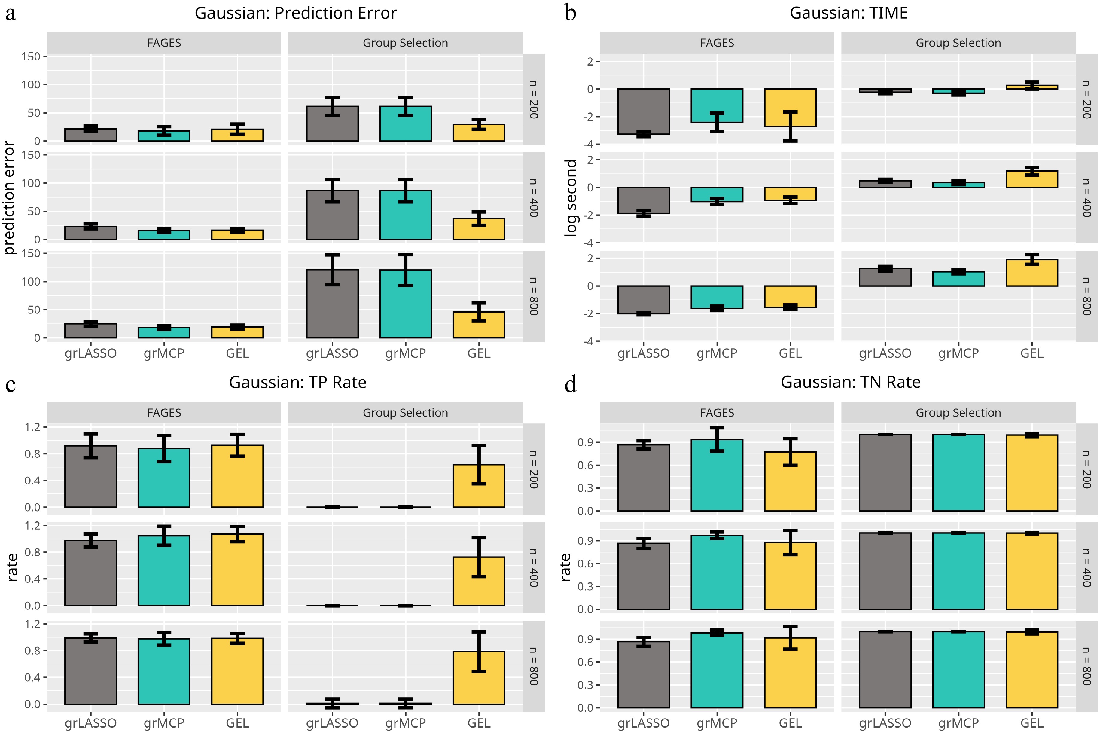corresponding to Scenario 1 or Scenario 2, respectively. The results shown in Figs. 2 and 3 correspond to Scenario 1 and 2, respectively.

Figure 2. 

Results of the linear model with respect to Scenario 1. Each panel represents a different evaluation metric: (a) prediction error, (b) computing time, (c) true negative rate, and (d) true positive rate. The height of each bar indicates the average value of the corresponding metric across multiple simulations, with error bars representing twice the standard deviation. The first three bars in each panel correspond to traditional methods, while the last three bars represent FAGES-based approaches with different penalty settings.

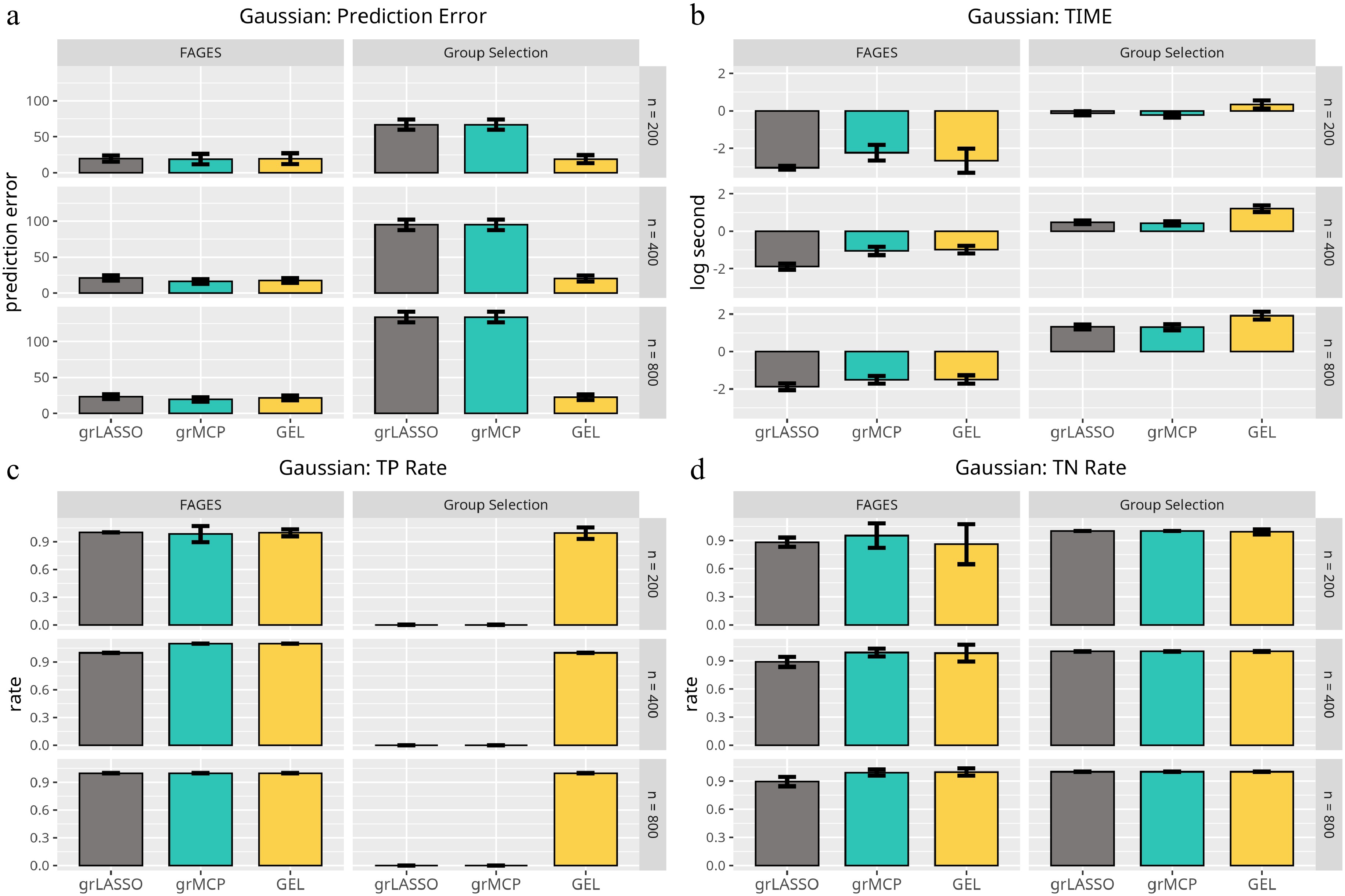
Figure 3. 

Results of the linear model with respect to Scenario 2. Each panel represents a different evaluation metric: (a) prediction error, (b) computing time, (c) true positive rate, and (d) true negative rate. The height of each bar indicates the average value of the corresponding metric across multiple simulations, with error bars representing twice the standard deviation. The first three bars in each panel correspond to traditional methods, while the last three bars represent FAGES-based approaches with different penalty settings.

Our findings from Fig. 2 are as follows. In terms of the PE, FAGES performs uniformly better than the traditional methods, regardless of the group variable selection penalty applied. Besides, the traditional method with GEL is the only accurate method. Groups LASSO and grSCAD cannot select any group when the group size is very large. In terms of computing time, FAGES is computationally efficient than the traditional ones since it reduces the dimension of the GLM by the PCA before minimizing it. Regarding the TN, both the traditional methods and FAGES show high accuracy when concave penalties are used. For the TP, FAGES shows the top performance, followed by the traditional method with GEL, while the remaining two traditional methods show no power. In addition, FAGES cannot achieve the group selection consistency with the group LASSO penalty because this penalty lacks the oracle property^[1].

In Fig. 3, we observe the following phenomena when the grouped factor-augmented GLM is misspecified. Traditional methods with GEL and FAGES are almost of the same accuracy in terms of PE. This phenomenon illustrates that FAGES is robust even when the underlying model is misspecified. As for TN and TP, the traditional approaches with GEL and FAGES are of the same accuracy. Regarding the computing time, FAGES is much faster than all three traditional methods, since it handles a model with a much lower dimension than the traditional methods. In summary, FAGES is still accurate when the underlying model is totally misspecified. In contrast, the traditional method performs well only when the GEL penalty is employed.

Example 2: Logistic regression

Now we investigate FAGES for binary responses under the logistic model: $ {{\rm{E}}}({\bf{y}})=\exp({\boldsymbol{\eta}})/\{1+\exp({\boldsymbol{\eta}})\} $, where $ {\boldsymbol{\eta}}={\bf{F}}{{\boldsymbol{\theta}}}^\star $ in Scenario 1 and $ {\boldsymbol{\eta}}={\bf{X}}{{\boldsymbol{\beta}}}^\star $ in Scenario 2. For binary outcomes, we observed that the group-penalized fitting in $\mathrm{grpreg}$ can be numerically unstable and may fail to converge, reflecting the fact that binary responses typically carry less information than Gaussian responses. To stabilize the optimization, we therefore use an elastic-net-type composite penalty by adding a ridge component with mixing parameter α in the minimization of θ. For the traditional approaches, we set α = 0.7, which we found yields stable computation and avoids the extremely low TP rates that arise when the ridge penalty is omitted, in which case most groups are not selected. FAGES exhibits the same issue but to a lesser extent; accordingly, we use a slightly larger value α = 0.8 to place less weight on the ridge penalty to reduce the bias. See $\mathrm{grpreg}$ for implementation details.

From Fig. 4, we learn that FAGES uniformly outperforms the traditional methods in terms of all four criteria when the underlying model is correctly specified. However, it should be noted that, despite the fact that traditional approaches perform far worse even when GEL is applied as a group selector, FAGES does not produce ideal results because it is likely to ignore groups with non-zero effects. Only when n is sufficiently large can FAGES achieve the model selection consistency. Fig. 5 illustrates that FAGES is more accurate than the traditional methods in terms of the PE, even when the underlying model is misspecified. The underlying explanation for this occurrence is that the binary response carries less information than the continuous response and thus, it prefers the model with less degrees of freedom, even if the other model with more degrees of freedom is closer to the true model. Hence, we conclude that FAGES is powerful and robust to analyze the high-dimensional grouped variables, especially for the binary response, as FAGES is able to greatly reduce the dimension of the conventional GLM (Eq. [3]) without losing any key information.

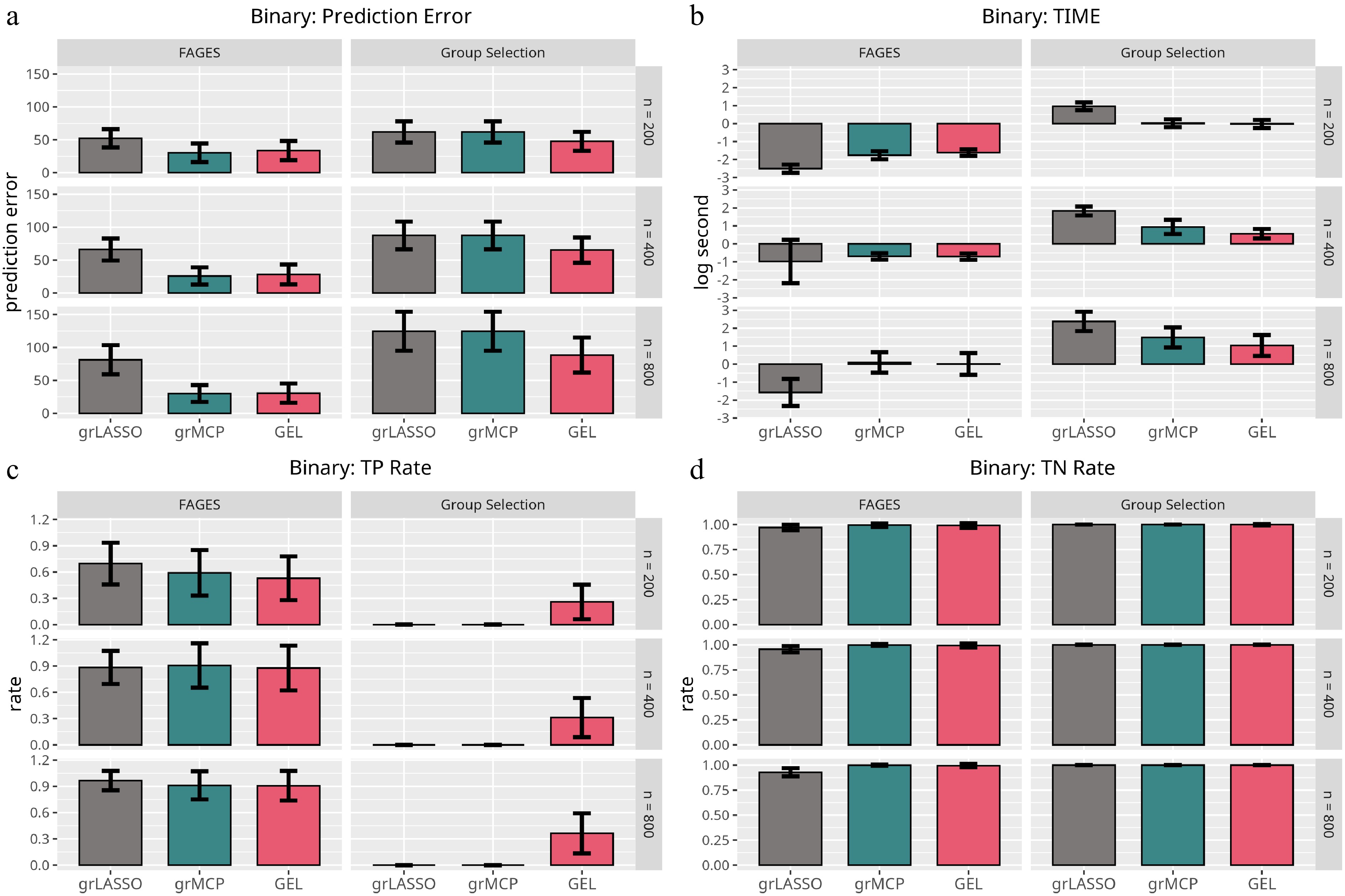
Figure 4. 

Results of the logistic model with respect to Scenario 1. Each panel represents a different evaluation metric: (a) prediction error, (b) computing time, (c) true positive rate, and (d) true negative rate. The height of each bar indicates the average value of the corresponding metric across multiple simulations, with error bars representing twice the standard deviation. The first three bars in each panel correspond to traditional methods, while the last three bars represent FAGES-based approaches with different penalty settings.

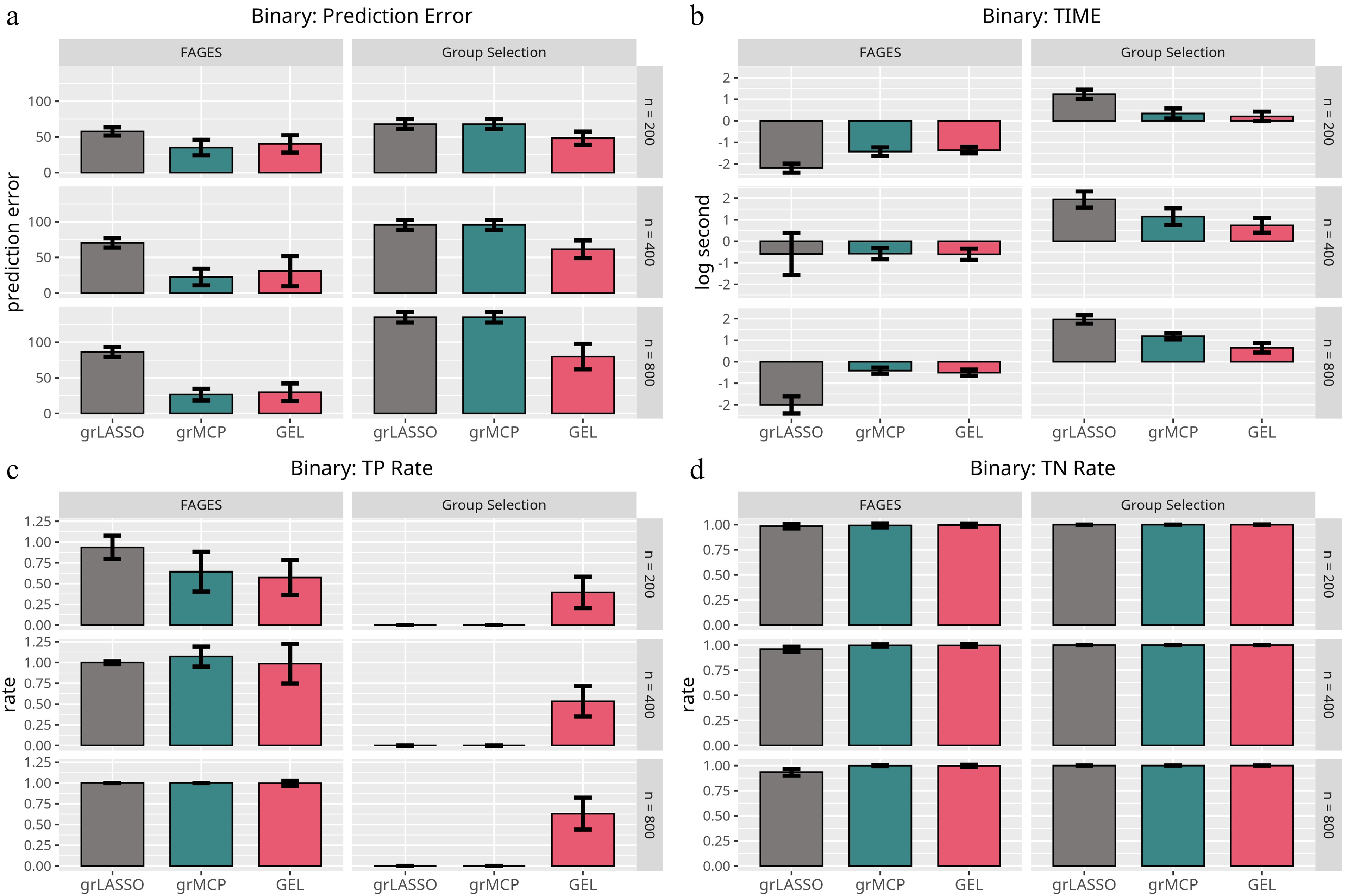
Figure 5. 

Results of the logistic model with respect to Scenario 2. Each panel represents a different evaluation metric: (a) prediction error, (b) computing time, (c) true negative rate, and (d) true positive rate. The height of each bar indicates the average value of the corresponding metric across multiple simulations, with error bars representing twice the standard deviation. The first three bars in each panel correspond to traditional methods, while the last three bars represent FAGES-based approaches with different penalty settings.

Example 3: Functional regression

We consider a more complex case: the observed variables of each group are in the form of smooth functions. Consider the following functional AFM:

where, t = (t₁, …, t_p)^T is a covariate like the time of observation, λ₁(t) is a smooth function of t, and $ {\boldsymbol{\Lambda}}({\boldsymbol{t}})=({\boldsymbol{\lambda}}_1({\boldsymbol{t}}),\dots,{\boldsymbol{\lambda}}_K({\boldsymbol{t}}))^\top $. In this case, the factor loading is considered a coordinate axis and the latent factor is viewed as the vector of random coordinates in this axis. To borrow information from the functional structure of $ {\boldsymbol{\Lambda}}({\boldsymbol{t}}) $, Fan et al.^[16] suggested first smoothing the observations X(t) by using a projection matrix P(t) and then yielding the consistent estimator of F and $ {\boldsymbol{\Lambda}}({\boldsymbol{t}}) $ through the PCA. This method is known as the projection-PCA method. As for the choice of P(t), one may employ the Tikhonov bases if t₁, …, t_p are regularized in interval [0, 1]. Let $ {\boldsymbol{p_s}}({\boldsymbol{t}})=\sqrt{2}\cos(s\pi {\boldsymbol{t}}) $ and $ {\boldsymbol{p}}({\boldsymbol{t}})=({\bf{1}},{\boldsymbol{p}}_1({\boldsymbol{t}}),\dots,{\boldsymbol{p_S}}({\boldsymbol{t}})) $, where S is a given cutoff. Then $ {\bf{P}}({\boldsymbol{t}})={\boldsymbol{p}}({\boldsymbol{t}}){\boldsymbol{p^\top}}({\boldsymbol{t}})/p $. For a suitable choice of $ S $, for example, S = 9, it is guaranteed that $ {\boldsymbol{\Lambda}}^\top({\boldsymbol{t}}){\bf{P}}({\boldsymbol{t}})\approx{\boldsymbol{\Lambda}}^\top({\boldsymbol{t}}) $ and $ {\bf{e}}{\bf{P}}({\boldsymbol{t}})\approx0 $^[34]. As a result, analyzing the projected data $ \hat{{\bf{X}}}={\bf{X}}({\boldsymbol{t}}){\bf{P}}({\boldsymbol{t}}) $ is an approximately noiseless problem, i.e.,

Similar to the ordinal AFM, the first $ K $ eigenvectors of $ \hat{{\bf{X}}}\hat{{\bf{X}}}^\top/n $ form the estimator of $ \hat{{\bf{F}}}/\sqrt{ n} $, and $ \hat{\Lambda}({\boldsymbol{t}})=\hat{{\bf{X}}}^\top\hat{{\bf{F}}}/\sqrt{n} $ is the latent loading estimator.

Without losing generality, we set $ p_1=\cdots=p_J $ = 2,000, and other parameters remain the same as in the previous simulations. Although the number of real observation points of a curve may be larger than 20,000, our experience shows it is sufficient to accurately estimate the function by using 2,000 points randomly sampled from the 20,000. We apply the projection-PCA to smooth the sample matrix $ {\bf{X}}_{{\cal{M}}_j}({\boldsymbol{t}}) $ by using the projection matrix $ {\bf{P}}({\boldsymbol{t}})={\boldsymbol{p}}({\boldsymbol{t}}){\boldsymbol{p^\top}}({\boldsymbol{t}})/p $, where $ {\boldsymbol{p}}({\boldsymbol{t}})=({\bf{1}},{\boldsymbol{t}}_1({\boldsymbol{t}}),\dots,{\boldsymbol{t}}_9({\boldsymbol{t}})) $ is the matrix of the Tikhonov basis functions. The latent factor $ \hat{{\bf{F}}}_{{\cal{M}}_j} $ is estimated from the smoothed matrix $ \hat{{\bf{X}}}_{{\cal{M}}_j}={\bf{X}}_{{\cal{M}}_j}({\boldsymbol{t}}){\bf{P}}({\boldsymbol{t}}) $ through the minimization (Eq. [2]). Here, we do not compare FAGES with the traditional group variable selection methods since the observation points of each function may be very large, in which case the traditional methods are very likely to fail.

The top three rows of Fig. 6 show the results of the linear model for functional data analysis. FAGES is clearly capable of handling the data that are in the form of smooth curves. FAGES accomplishes the model selection consistency with a high probability using the concave penalty no matter the sample size is large or small. The bottom three rows of Fig. 6 present the counterpart of the logistic regression model. FAGES is likely to ignore certain non-zero groups, consistent with the previous simulations. Only when the sample size is sufficiently large can FAGES achieve the model selection consistency.

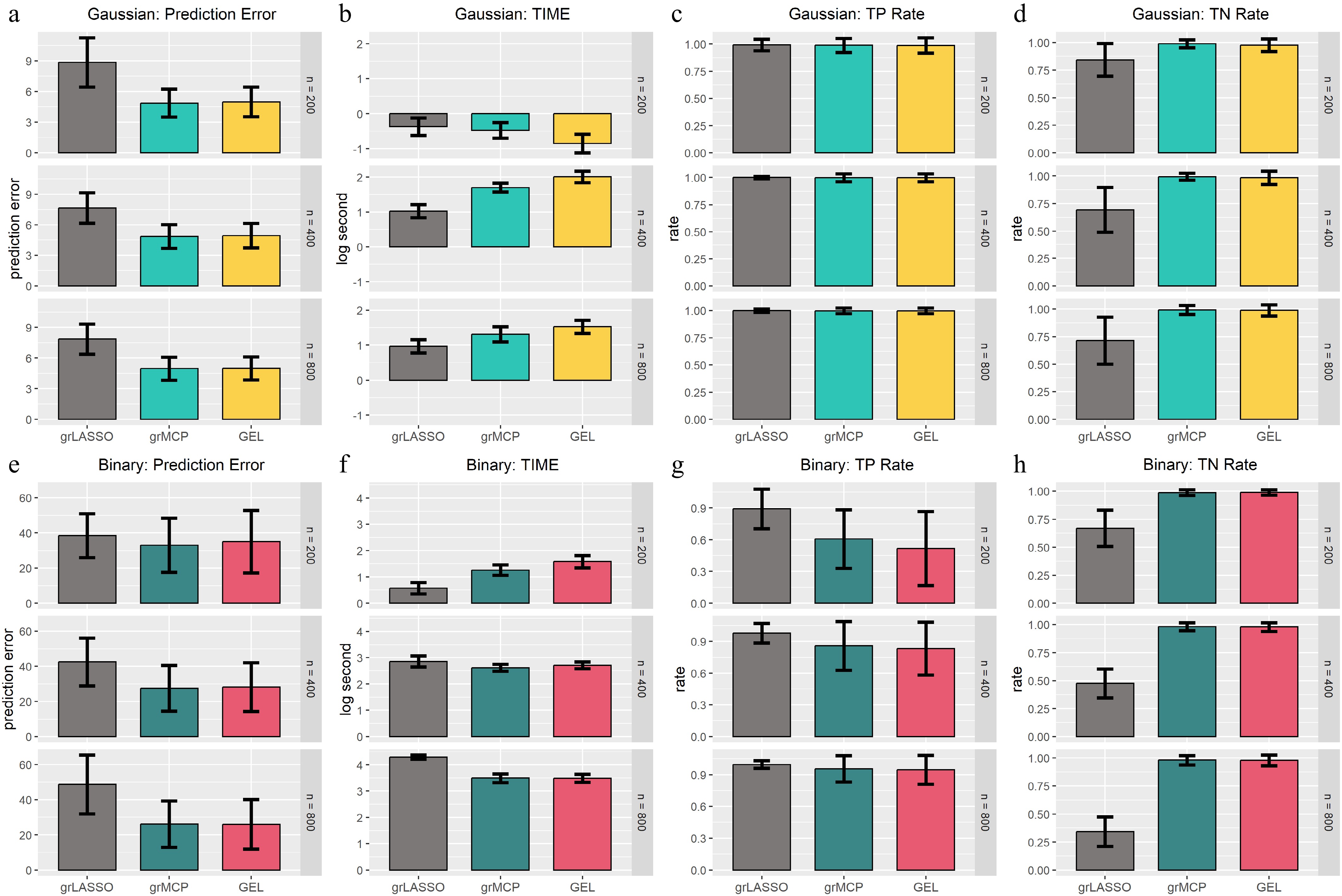
Figure 6. 

Results of functional data analysis. The first four rows correspond to the Gaussian model, while the last four rows correspond to the binary model. Each column represents a different evaluation metric: (a), (e) prediction error; (b), (f) computing time; (c), (g) true negative rate; and (d), (h) true positive rate. The height of each bar indicates the average value of the corresponding metric across multiple simulations, with error bars representing twice the standard deviation. Different methods are compared, with the first set of bars corresponding to traditional approaches and the latter set representing FAGES-based methods with different penalty settings.

Real-data analysis

Data

In this section, we demonstrate the analysis of the HNSCC data through FAGES. We first give a description of the data and related concepts and then show the results of the analysis. The HNSCC data are provided by the cancer genome atlas (TCGA) program and can be found on the website UCSC Xena (https://xenabrowser.net/datapages). The website contains data related to n = 520 patients and 20,530 genes, which show the gene-level transcription estimates, as in the log₂(x+1)-transformed RSEM normalized count. The gene "Ki67" is considered the response variable because it is the indicator gene in many biological researches. For example, "Ki67" may be necessary for cellular proliferation; it is involved in maintaining the individual mitotic chromosomes dispersed in the cytoplasm following nuclear envelope disassembly; and higher expression of "Ki67" is related to a poor prognosis of cancer^[35,36].

A pathway is a kind of gene set commonly used in biological researches. There are more than 20,000 genes in humans, and their molecular functions are based on the so-called biological pathways, which host a series of interactions among genes or molecules in a cell that lead to a biological function. KEGG is a kind of pathway database built for understanding the high-level functions and utilities of the biological system from gene-level or molecular-level information, especially large-scale molecular datasets generated by genome sequencing and other high-throughput experimental technologies^[37].

The KS random walk method^[9] is applied to convert the gene expressions into an individualized KS curve that reflects the enrichment of a target gene set. Suppose there is a matrix of expression profiles $ {\bf{V}}=(V_{ij})_{n\times p} $, where n is the number of samples and p is the number of genes. The KS random walk method first ranks the V_ij for every sample to obtain the rank statistics S_ij and then yields the KS curve using the accumulation process

where, $ {\bf{1}}(h\in{\cal{M}}_j) $ is the indicator function that shows whether the h-th gene (the gene corresponding to the h-th ranked expression-level statistic) belongs to gene set $ {\cal{M}}_j $, $ |{\cal{M}}_j| $ is the number of genes in the $ j $-th gene set, and p is the number of genes in the gene data. For l = 1, …, p, the KS statistics $ {\boldsymbol{X}}_{il,{\cal{M}}_j} $ form an individualized KS curve corresponding to gene set $ {\cal{M}}_j $.

Analysis

We consider the KEGG pathways as gene sets and utilize the KS random walk approach to generate the individualized KS curves for every pathway. Besides, we assume the individualized KS curves to follow an AFM (Eq. [7]) in each pathway, and use the projection-PCA to estimate the related latent factor. Without loss of generality, the dimensions of the latent factors are uniformly set as 3 and only the 1st,..., 1027th quantiles of each KS curve are recorded. We use the penalized likelihood (Eq. [15]) to handle the grouped factor-augmented GLM (Eq. [8]). The averaged group effect is computed through Eq. (16) and the effect direction is determined based on Eq. (17).

Figure 7 demonstrates the identified pathways and the related pathway effects using FAGES. First of all, FAGES with the two different penalties identifies many consistent pathways, including Toxoplasmosis, TGF-beta, Staphylococcus aureus infection, Progesterone edited oocyte maturation, etc. Besides, FAGES with the GEL identifies ten more important pathways than FAGES with the grMCP because of GEL's flexibility. The cell cycle and TGF-beta are the two pathways that have the most significant averaged group effects in both methods. The cell cycle pathway, which regulates DNA synthesis and mitosis during tumor cell proliferation, is recognized to be positively associated with tumor cell proliferation^[38]. The TGF-beta pathway, consistent with previous reports, has a strongly negatively averaged group effect on cell proliferation, implying that the activation of this pathway might compromise tumor proliferation^[39]. Furthermore, pathways with considerable averaged group effects, such as prostate cancer, toxoplasmosis, amino sugar and nucleotide sugar metabolism, and inositol phosphate metabolism, warrant further investigation. In this process, FAGES acts as a screen that removes the noisy genes in a more statistically valid and biologically understandable manner.

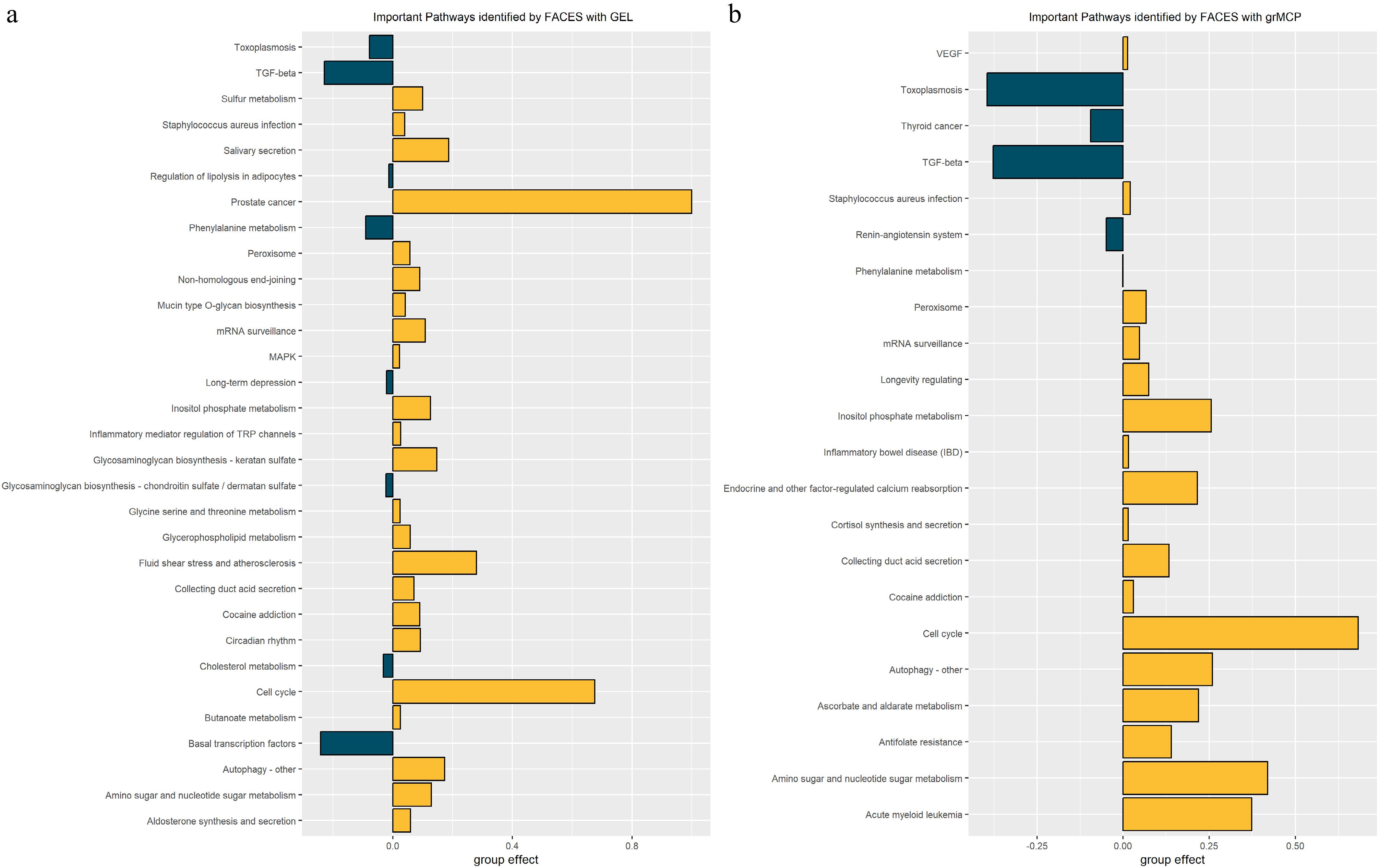
Figure 7. 

Important pathways identified by FAGES with different penalty functions. (a) shows the results obtained using GEL, while (b) displays the results yielded by grMCP. The bars represent the estimated averaged group effect for each selected pathway, with the pathway names shown on the y-axis. Green bars indicate pathways that are positively associated with the outcome, while yellow bars indicate pathways that are negatively associated with the outcome.

In this paper, we introduce a two-stage method called FAGES for identifying important variable groups within the framework of GLM. Methodologically, FAGES first addresses within-group correlations by modeling each group of variables with an AFM. Each group is assumed to be driven by a few latent factors together with idiosyncratic components, with the latent factors capturing the dominant variation^[18]. By representing groups through their latent factors, FAGES reduces dimensionality and specifies a grouped factor-augmented GLM in which these latent factors are entered as predictors associated with the outcome. A variable selection penalty is then applied to simultaneously identify relevant groups and estimate their corresponding regression coefficients. For inference, FAGES quantifies the strength of the selected groups through an averaged group effect estimate (Eq. [16]), which provides a comparable measure of the group contribution.

In our simulations, we found that grMCP performs slightly better than GEL. This is not surprising. Under idealized settings, grMCP does not impose an explicit bi-level selection structure and can therefore exploit the group information more efficiently, which may translate into higher power. However, prior empirical evidence in the literature suggests that, in real-data applications, GEL tends to be more robust to heterogeneous within-group correlation patterns and model misspecification^[8]. Hence, we recommend GEL as the default choice in practice, and view grMCP as a competitive alternative when the signal is sufficiently strong and the group structure is well aligned with the assumed model.

As an application of FAGES, we show how to enhance GSVA by using FAGES in real-data analysis. Traditional GSVA relies on a single summary statistic, such as the maximum deviation or maximum difference statistic, to extract information from the KS curve^[9]. We propose leveraging the leading FPCs of the KS curve to more effectively capture the contribution of gene sets to the outcome, and estimate the direct effect of a gene set on the outcome conditional on other gene sets. Beyond this application, we further hypothesize that FAGES can benefit Mendelian randomization (MR) analyses based on rare variants^[40,41]. Specifically, we propose to ① construct a weighted kernel matrix for rare variants within a genomic region based on SKAT^[42], and ② apply PCA to extract the leading kernel-weighted PCs. Furthermore, we can ③ select key genomic regions and estimate the effects of their PCs on both the exposure and the outcome, which can serve as instrument variables (IVs) in MR, and ④ ultimately perform MR to assess whether the exposure causally influences the outcome through the rare variants. For example, rare loss-of-function variants in ANGPTL3 have been associated with a decreased risk of cardiovascular diseases^[43], while the common cis protein quantitative trait locus (pQTL) of ANGPTL3 abundance showed no causality^[44]. In the future, we can investigate whether lipid traits, such as triglyceride, mediate their effect on ASCVD through rare loss-of-function ANGPTL3 variants by using a FAGE-based MR analysis.

Several limitations of the present study should be acknowledged. First, in the real-data analysis, we chose Ki67 expression as the response variable. Although Ki67 is a well-established marker of cellular proliferation and is widely recognized as a prognostic indicator in oncology^[35,36], modeling the expression level of a single gene is less conventional in GSA. Thus, this application should be viewed mainly as a proof-of-concept illustration of FAGES. Second, the two-stage estimation procedure, which first extracts latent factors and then applies penalized regression, may introduce additional variability and potential heteroskedasticity^[45]. Moreover, we did not include direct comparisons with classical GSA methods (e.g., AUCell^[46] and PAGODA^[47]), because these approaches are marginal by design, while our aim is to advance group variable selection methods that estimate the conditional effects in a regression framework.