Progress and perspectives on genomic selection models for crop breeding

The development of new crop varieties through breeding is an efficient way to enhance crop productivity. Breeders aim to improve breeding traits of interest such as yield, disease resistance, stress tolerance, and nutritional value. Modern crop breeding is both an art and a science, and is vastly different from early crop selection and domestication due to the rapid development of scientific techniques such as biostatistics, genetic engineering, and genomics and to advancements in various modern breeding techniques, including transgenesis, genome editing, speed breeding, and doubled haploid (DH) technology^[1]. As a result, modern breeding is entering a novel stage, Breeding 4.0, based on the proposed stages of agriculture from 1.0 to 4.0^[1].

Two major strategies are employed in molecular breeding: marker-assisted selection (MAS), and genomic selection (GS)^[2]. During MAS, each individual plant is identified based on linked or functional markers that confirm the trait of interest^[3]. Owing to the discovery of increasing numbers of major quantitative trait loci (QTLs) and functional genes through genetic research, MAS has been extensively applied in different types of breeding programs to improve traits of interest since its initial use in the 1990s^[3]. MAS is an effective way to increase selection efficiency for qualitative traits or categories of traits that are regulated by only a few genes^[4]. However, important traits targeted by breeding that are regulated by one or a few major QTLs/genes are extremely rare. Most traits, such as yield and plant height, are quantitative traits that are regulated by multiple loci. As it is challenging to conduct artificial selection using only a few markers to identify the genes underlying traits of interest, a second strategy known as GS (also known as whole-genome prediction) was developed^[5].

In breeding programs, much effort was focused on predicting the breeding value of a specific material even before the emergence of GS. One approach that breeders have explored is predicting the performance of the progeny of single crosses. However, predicting the performance of the progeny of single crosses can be complex due to the presence of a genetic network, including factors with dominant or epistatic effects, especially for complex quantitative traits^[6]. With the emergence of molecular biology techniques, DNA molecular markers have been developed and used in breeding programs. Researchers have started to incorporate these markers into regression models to estimate the breeding value of breeding materials. The use of DNA markers is effective for increasing the genetic gain, with improvements ranging from 8% to 38% in various studies^[3,7]. Simultaneously, with advancements in marker technology, it has become feasible to produce markers rapidly at a lower cost, opening new avenues for incorporating genomic information into breeding programs^[8].

GS involves predicting the breeding value of a material using information from a large number of genetic markers distributed across the genome. This technique was formally proposed by Meuwissen et al. in 2001, who proved that it was possible to predict breeding value using Bayesian and BLUP (best linear unbiased prediction) statistical models^[5]. GS involves three major steps: construction of the training dataset, optimization of the model and parameters, and prediction of the evaluation dataset. These steps collectively form the basis of the GS workflow (Fig. 1a). However, the development of each step faced various challenges before yielding promising results. For instance, GS was not incorporated into breeding programs in the early 2000s due to the limited number of molecular markers available and the high cost of marker testing^[9]. The emergence of high-throughput marker testing platforms, such as single-nucleotide polymorphism (SNP) arrays, DNA microarrays, and second- and third-generation sequencing technologies, has enabled breeders to genotype numerous individuals efficiently at low cost, facilitating the widespread adoption of GS in breeding programs^[10]. Subsequently, GS has become an increasing focus of research and development in breeding.

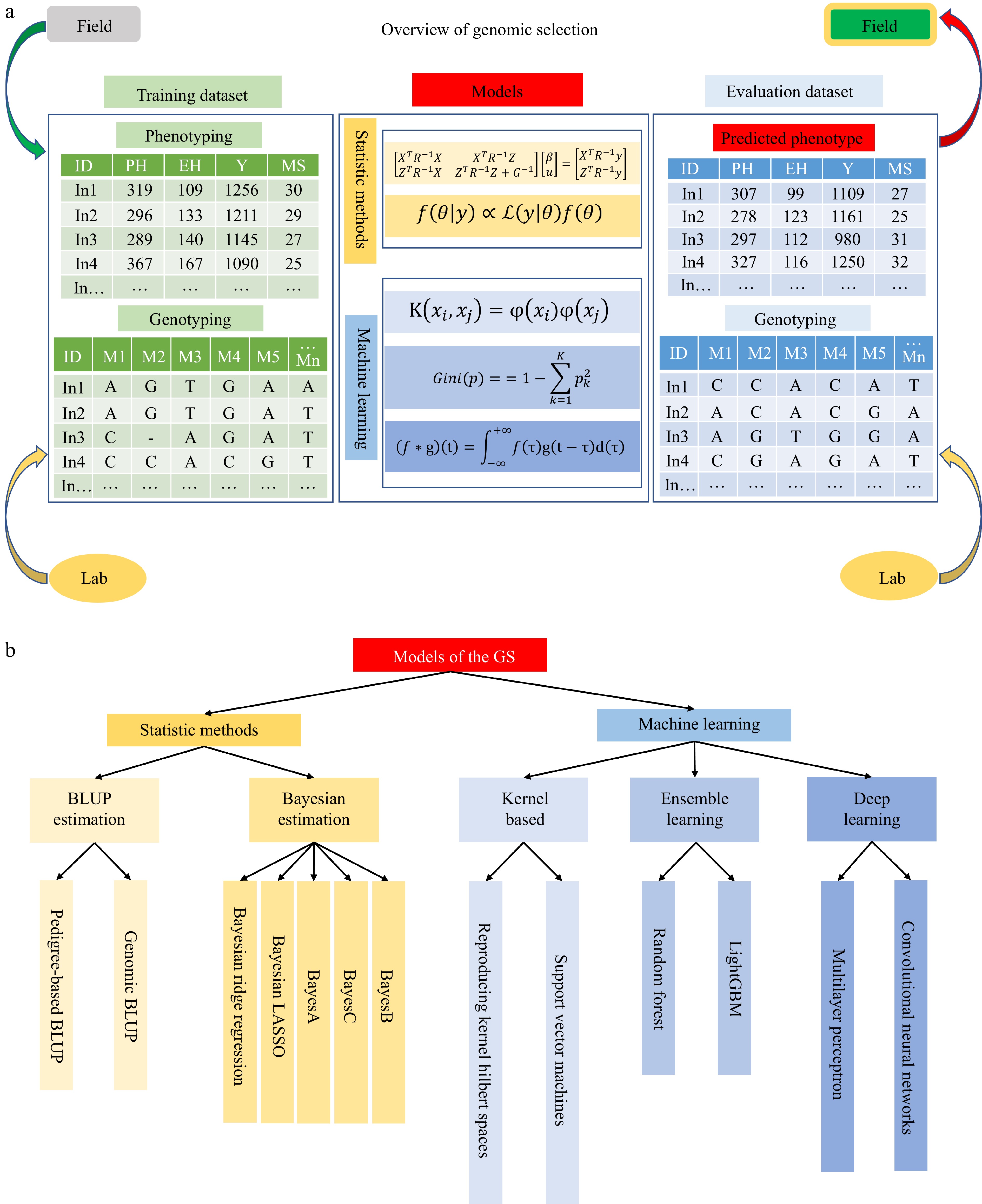
Figure 1. 

An overview of genomic selection. (a) There are three parts in the genomic selection, including the training dataset, models, and evaluation dataset. The training dataset consists of phenotyping data collected from the field trials and genotyping data tested in the marker lab. The models are trained through two strategies: statistical methods and machine learning. The evaluation dataset is predicted phenotype and genotyping. The materials would be selected according to the predicted phenotyping and then go to field experiments. (b) Summary of models in GS.

With the accumulation of genotypic and phenotypic data, the use of GS for molecular breeding has made significant contributions to breeding within major plant breeding companies, especially for screening DHs and hybrid prediction^[11]. Many models continue to be proposed and improved to enhance the accuracy of prediction. Below, we describe various models from statistics and machine learning (ML) and review them in detail (Fig. 1b).

Before genomic relationships were used for GS, pedigrees were used to predict the breeding values of individual crop plants via BLUP mixed-model equations. It is straightforward to determine phenotypic similarity when the progenies share the same pedigree information, which enhances the efficiency of artificial selection^[12]. However, this method cannot be used by breeders when pedigree information is lacking or progenies are derived from the same parents (i.e., a full-sib family). Therefore, scientists explored ways to more accurately assess the kinship of individuals based on their genomic relationships with the advent of DNA molecular markers.

GBLUP were used to predict the breeding values of individual crop plants via BLUP mixed-model equations. BLUP estimation is derived from the linear mixed model and the following mixed-model equation:

where, $ {\sigma }_{g}^{2} $ is the total genetic variance, $ {\sigma }^{2} $ is the random error variance, $ \lambda =\dfrac{{\sigma }^{2}}{{\sigma }_{g}^{2}} $, $ R $ is the random error variance–covariance coefficient matrix $ I $, and $ G $ is the genetic variance–covariance coefficient, which is derived from the estimation of genomic relationships^[13,14] as follows:

where, Z is the matrix of all markers, p_i is the frequency of each marker, and all other parameters are identical. The ability to estimate genomic relationships is a critical measure for improving the prediction accuracy of GBLUP. Therefore, various methods have been introduced for estimating genomic relationships^[14,15] including single-step GBLUP (ssGBLUP), which combines pedigree-kinship information with genomic relationship information to estimate genomic relationships^[16,17]. Subsequently, additional GBLUP methods have emerged.

In trait-specific marker-derived relationship matrix (TABLUP), another GBLUP method, a trait-specific relationship matrix is built based on the identity by descent (IBD) between both individuals from the locus with the genetic variance in the trait^[18]. The equation is as follows:

where, k is the locus, $ {P}_{IBD,ijk} $ is the probability of IBD, i and j are individuals, $ {\sigma }_{g}^{2} $ is the genetic variance of the trait, and kinship is the sum of values for all loci. Subsequently, Wang et al. proposed two more methods: SUPER BLUP (sBLUP) and compressed BLUP (cBLUP)^[19], which were derived from the GWAS (genome-wide association study) theory. In sBLUP, the kinship matrix is designed by selecting significant bins, which are grouped based on the markers associated with traits of interest via GWAS^[20]. In cBLUP, all individuals are clustered into several groups according to their genomic relationships. The kinship matrix is the average of the genomic relationships^[21]. rrBLUP is a specific model used to implement kinship-based BLUP and SNP-based BLUP. With this method, the genomic relationship is calculated as $ {K}_{RR}=G{G}^{T} $, which is equivalent to the SNP-based rrBLUP methods^[22,23].

In BRR, the effect of all SNP markers is assigned to an identical and independent Gaussian prior distribution, and the beta coefficients used to describe the effect are at normal densities: $ \beta \sim \mathrm{N}(0,{\sigma }_{\beta }^{2}) $, where the prior distribution of the variance comes from the scaled inverse chi-square distribution, $ {\sigma }_{\beta }^{2}\sim{\chi }^{-2}\left({\upsilon }_{\beta },{S}_{\beta }\right) $; the hyperparameters $ {\upsilon }_{\beta } $ and $ {S}_{\beta } $ will be updated in the model^[24,25]. Under this hypothesis, all markers are linked with QTLs. However, in practice, not all markers have a phenotype effect. As a result, other prior distributions have been proposed to solve this problem.

Bayesian LASSO (BL)

The Bayesian form of LASSO infers variants according to the prior density of double-exponential distribution^[26,27]. Here, beta coefficients of the effect are at normal densities, $ \beta \sim\mathrm{N}(0,{\tau }_{p}^{2}{\sigma }^{2}) $. The variance is scaled-inverted chi-square density with degrees of freedom $ \upsilon $ and scale $ S $, $ {\sigma }^{2}\sim{\chi }^{-2}(\upsilon ,S) $. $ {\tau }_{j}^{2}\sim\mathrm{E}xp\left(\lambda \right) $ is an exponential density with the hyperparameter $ \lambda $, $ {\lambda }^{2}\sim Gamma({\alpha }_{1},{\alpha }_{2}) $ is a gamma distribution with two hyperparameters: shape parameter $ {\alpha }_{1} $ and rate parameter $ {\alpha }_{2} $. There are two other $ \lambda $ prior distributions: $ {\lambda }^{2}\sim beta(p,\pi ) $ and a flat distribution^[25,28]. Moreover, Legarra et al. proposed BL2Var, with coefficient $ {\tau }_{j}^{2} $: $ {\tau }_{j}^{2}\sim\mathrm{I}\mathrm{G}\left(\sqrt{\dfrac{{\tilde{\lambda }}^{2}}{{\tilde{a}}_{i}^{2}}},{\lambda }^{2}\right) $, and BL1Var, with coefficient $ {\tau }_{j}^{2} $: $ {\tau }_{j}^{2} \sim\mathrm{I}\mathrm{G}\left(\sqrt{\dfrac{{\tilde{\lambda }}^{2}{\sigma }^{2}}{{\tilde{a}}_{i}^{2}}},{\lambda }^{2}\right) $^[29].

BayesA

In BayesA, the variances of each marker effect are different genome-wide, with a scaled inverse chi-square distribution: $ {\sigma }_{{\beta }_{j}}^{2}\sim{\chi }^{-2}({\upsilon }_{\beta },{S}_{ \beta }) $; $ {\upsilon }_{\beta }=4.012 $ and $ {s}_{\beta }= $ 0.0020 are the suggested fixed values for the degrees of freedom and scaled parameter, respectively. As a result, a scaled-t density could explain the marginal distribution of marker effects^[5]. However, the shrinkage of SNP effects is severely affected by $ {S}_{ \beta } $, which should be considered as an unknown parameter with its own prior $ {S}_{ \beta }\sim Gamma\left(r,s\right) $; $ r $ and $ s $ are rate parameter and shape parameter, respectively^[30].

BayesC

In BayesC, the variances of all marker effects are identical and independent, with a prior scaled inverse chi-square distribution: $ {\sigma }_{\beta }^{2}\sim {\chi }^{-2}({\upsilon }_{\beta },{S}_{ \beta }) $; $ {\upsilon }_{\beta } $ and $ {S}_{ \beta } $ are the degrees of freedom and scaled parameter, respectively. $ {S}_{ \beta } $ has a prior density: $ {S}_{ \beta }\sim Gamma\left(r,s\right) $; $ r $ and $ s $ are the rate and shape parameters, respectively. The beta coefficients of the effect are normal density: $ {\beta }_{j}\sim N(0,{\sigma }_{\beta }^{2}) $ with probability $ \pi $, $ {\beta }_{j}=0 $ with probability $ 1-\pi $. Additionally, $ \pi $ is the prior density: $ beta(a,b) $, when $ \pi $ is suggested as the unknown parameter with a prior density $ beta(a,b) $, which is referred to as BayesCπ^[30].

BayesB

BayesB combines the hypotheses from BayesA and BayesC. First, the beta coefficient of the effect is normal density: $ {\beta }_{j}\sim N(0,{\sigma }_{{\beta }_{j}}^{2}) $ with probability $ \pi $, and $ {\beta }_{j}=0 $ with probability $ 1-\pi $. Additionally, $ \pi $ is the prior density: $ beta(a,b) $, when $ \pi $ is suggested as the unknown parameter with a prior density $ beta(a,b) $, which is referred to as BayesDπ. The variances of each marker effect are different genome-wide, with a scaled inverse chi-square distribution: $ {\sigma }_{{\beta }_{j}}^{2}\sim {\chi }^{-2}({\upsilon }_{\beta },{S}_{ \beta }) $, $ {S}_{ \beta }\sim Gamma\left(r,s\right) $; $ r $ and $ s $ are rate parameter and shape parameter, respectively^[5,25].

Several other Bayesian estimations can be used for different prior distributions on marker effects, including BayesU^[31], BayesHP, BayesHE^[32], BayesR, and emBayesR^[33]. Based on the above descriptions, Bayesian theory could provide a series of models for GS given different prior hypotheses. A mixture of prior distributions is used to generate many diverse types of models by combining the different prior hypotheses. The mean and variance of all parameters could be estimated by Markov chain Monte Carlo of Metropolis-Hastings or Gibbs sampling^[34] and the prediction accuracy of these models is comparable to that of other models^[35].

Although the accuracy of phenotypic prediction during GS has improved, it remains challenging to analyze highly complex agronomic traits regulated by numerous genetic loci with minor effects^[36]. This makes it difficult to depict the genetic interactions from models via classical BLUP estimation or Bayesian estimation^[37]. Furthermore, epistatic effects and imprinting of genetic interactions are common and widely present within biological processes^[38]. Consequently, ML methods have been proposed to address the problems arising from genetic interactions using non-linear approaches^[39,40]. Much effort has been devoted to developing ML methods to improve the accuracy of GS.

Kernel-based models

A kernel function (also known as 'the kernel trick') could be implemented to transform a vector of low-dimensional space into the inner product of a vector of infinite dimension. ML can be used for non-linear classification by implementing features from a low-dimensional space to be mapped into higher-dimensional feature spaces. Kernel functions show highly improved computational efficiency by specifically calculating functions in low-dimensional spaces:

where $ {x}_{i} $ and $ {x}_{j} $ are features of a low-dimensional space, and $ \varphi $ is the function for mapping $ {x}_{i} $ and $ {x}_{j} $ to a higher-dimensional feature space. Several kernel functions could be implemented for the computation of $ \varphi $, including linear kernel, polynomial kernel, sigmoidal kernel, and Gaussian kernel. These methods effectively capture the non-additive genetic effects among individuals for phenotypic prediction in biological statistics. In quantitative genetics, non-additive genetic effects play a critical role in elaborating the basic theory of genetic networks. High-dimensional genetic effects are rarely computed due to limited storage space and computing efficiency. The results of these models are expressed as an $ n\;\times\; n $ matrix via the kernel function. Additionally, some hyperparameters need to be trained.

Theoretical aspects of the reproducing kernel Hilbert space (RKHS) mixed model were introduced to study the non-linear relationships of genetic interactions through the kernel function in Hilbert spaces in 2006^[41]. In 2008, Gianola & Van Kaam expanded this technique, reproducing a mixed model of kernel Hilbert spaces that parsed epistatic variance between the effects of many genetic loci via a linear mixed model^[42]. The linear model of the dual formulation of RKHS is:

where $ \beta $ is the fixed variable; $ u $, $ \alpha $, and $ e $ are random variables with independent distributions; and $ u \sim N(0,{\sigma }_{g}^{2}G) $, $ \alpha |h \sim N(0,{\sigma }_{\alpha }^{2}{K}_{h}^{-1}), $ and $ e \sim N(0,{\sigma }^{2}I) $, respectively. Similarly, the regression estimating equation is:

where, $ R=I $; $ {K}_{h} $ is the correlation matrix from the results of the kernel function of features.

Subsequently, a general framework was proposed for the genetic evaluation of RKHS regression for pedigree- or marker-based regressions under any genetic model^[43]. Additionally, the Bayesian approach was formulated to solve the unknown parameter from the RKHS mixed model^[42,44]. RKHS regression outperformed the linear models in predicting the total genetic values of the body weight of chickens^[45].

Support vector machines (SVMs) are another set of efficient methods for non-linear classification through the kernel function^[46]. The model is:

where $ y $ is the response variable of the sample, $ \beta $ and $ b $ are the coefficients to be solved, and $ X $ is the feature variable. In the SVM model, the critical thought is a hyperplane that can separate a high-dimensional space into two parts. To guarantee the hyperplane's uniqueness, the points in a space must be at the maximum distance from this hyperplane, i.e., at the maximum margin hyperplane. The transformed formulation of the optimization is:

where $ {\xi }_{i} $ are slack variables and $ C $ is a regularization parameter. To achieve variables of the low-dimensional space to map to the high-dimensional space, a primal-dual method was used to solve optimization problems^[47,48]. The dual formulation is:

where $ {\alpha }_{i} $ is the variable parameter of dual formulation, $ \varphi ({x}_{i}{)}^{T}\varphi ({x}_{j})=K({x}_{i},{x}_{j}) $, which would be computed by the kernel function. The kernel function might be a polynomial kernel, sigmoidal kernel, Gaussian kernel, or other kernel type. The parameter $ \beta $ is expressed according to the following primal-dual formulation:

Finally, the decision function is:

Applying SVM to GS for trait prediction is a straightforward process and SVM is indeed a competitive and promising strategy for GS in plant breeding^[49,50]. On the whole, the decision function of the SVM depends on only a few support vectors, which is an advantage when classifying a small number of samples. Moreover, the complexity of the calculation is low to avoid a 'dimensionality disaster'.

Ensemble learning

Ensemble learning is a technical framework that is not a single ML algorithm per se. In ensemble learning, a learning task is accomplished by building and combining multiple basic machine models that decide the ultimate results. Ensemble learning can be used for classification, regression problems, and feature selection during data mining. This technique could be applied to GS to predict the phenotypic values of new individuals. Three common ensemble learning frameworks are currently used: bagging (also known as bootstrap aggregation), boosting, and stacking.

Random Forest (RF) is a typical bagging ML method (Fig. 2)^[51]. Using this method, M training samples are drawn from the N original sample set via the bootstrap method per round. In the training set, some samples may be drawn multiple times, while some samples may not be drawn even once. K rounds of extraction are carried out to obtain K training sets that are independent of each other. K training sets are constructed using different types of decision tree algorithms for classification or regression. For example, each weak learner could be constructed by classification and regression tree^[52] using the Gini index: $ \mathit{Gini}\left(p\right)=1-\sum_{k=1}^Kp_k^2 $.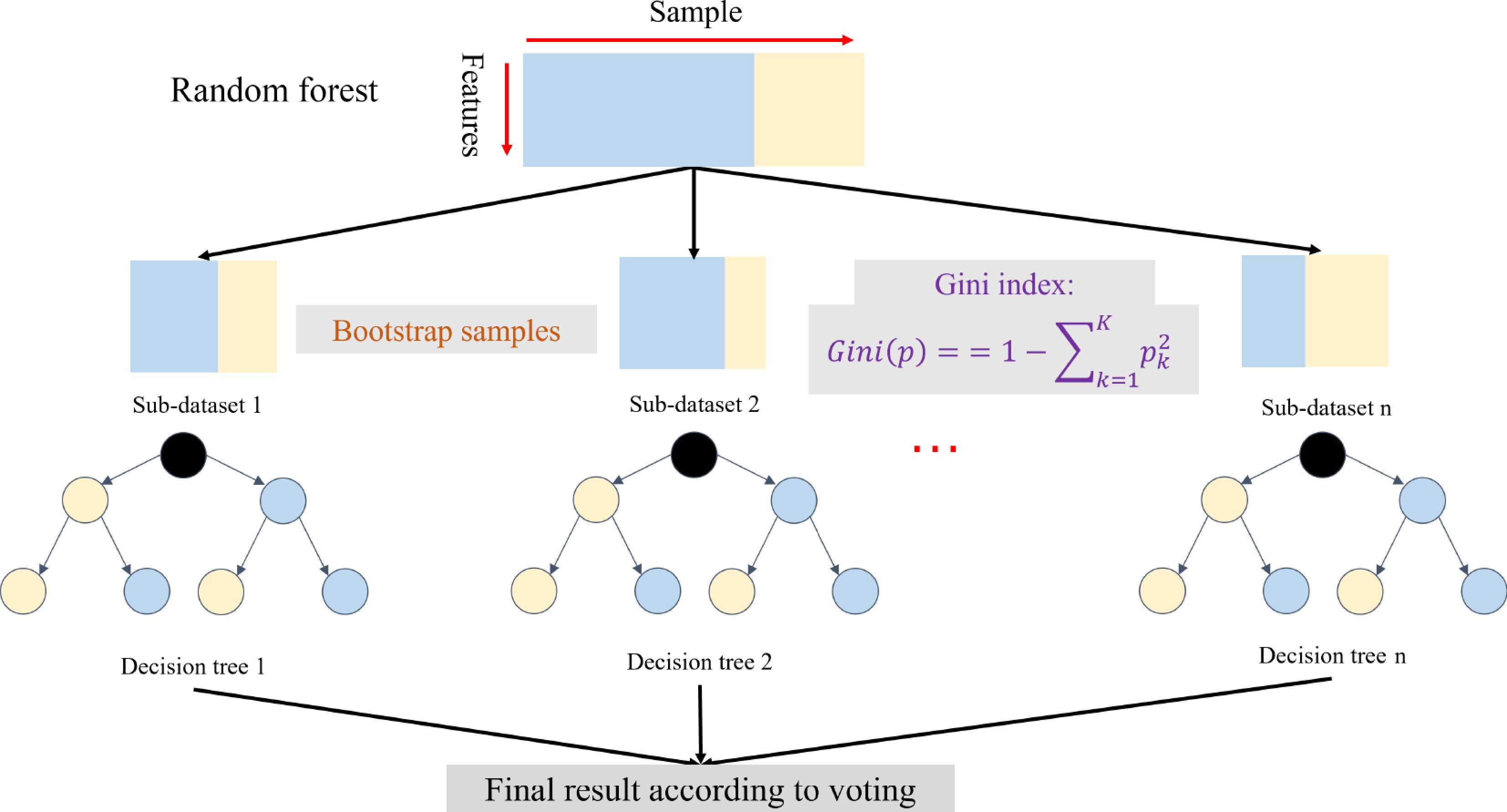

Figure 2. 

An overview of the random forest^[51]. The random forest includes the bootstrap samples and weak learners based on the decision tree with the Gini algorithm.

Theoretically, other ML algorithms could generate new weak learners according to the K training sets. Compared to the decision tree, RF has lower accuracy at the beginning of training, but its performance improves with increasing rounds of training. Therefore, RF is an outstanding method for ML and is starting to be used to analyze genetic networks, generating promising results^[53]. RF is a robust learner that reduces noise and overfitting in the GS model training process due to the use of nonparametric measures, but a large amount of data is needed to promote the efficiency of the GS model^[54]. Additionally, to analyze additive and epistatic effects and thereby improve the accuracy of GS, RF has been modified by combining it with a linear mixed model and a Bayesian model to construct a mixed RF model and Bayesian additive regression trees (BART)^[55].

Light gradient boosting machine (LightGBM): There are two major boosting methods: adaptive boosting (AdaBoost)^[56], and gradient boosting (GB)^[56]. Gradient boosting decision tree (GBDT) was originally developed from GB using a weak classifier CART decision tree^[56]. This tool uses weak classifiers to iteratively train and optimize the model, so that it has good prediction accuracy and easily avoids overfitting. LightGBM^[57], extreme gradient boosting (XGBoost)^[58], and categorical boosting (CatBoost)^[59] are thought to be the three best implementations of GBDT, as they outperformed the basic GBDT algorithm framework. XGBoost is widely applied in the industry, LightGBM has more effective computational efficiency, and CatBoost is thought to have better algorithm accuracy.

LightGBM employs some novel optimizations to accelerate calculations and reduce the need for memory storage and is therefore an improved version of XGBoost as well (Fig. 3)^[57]. This method extends the pre-sorted algorithm and histogram-based algorithm to preprocess the features of a dataset to reduce its complexity. A novel sampling algorithm, gradient-based one-side sampling (GOSS), was developed to decrease the size of the dataset without decreasing the accuracy of the model.

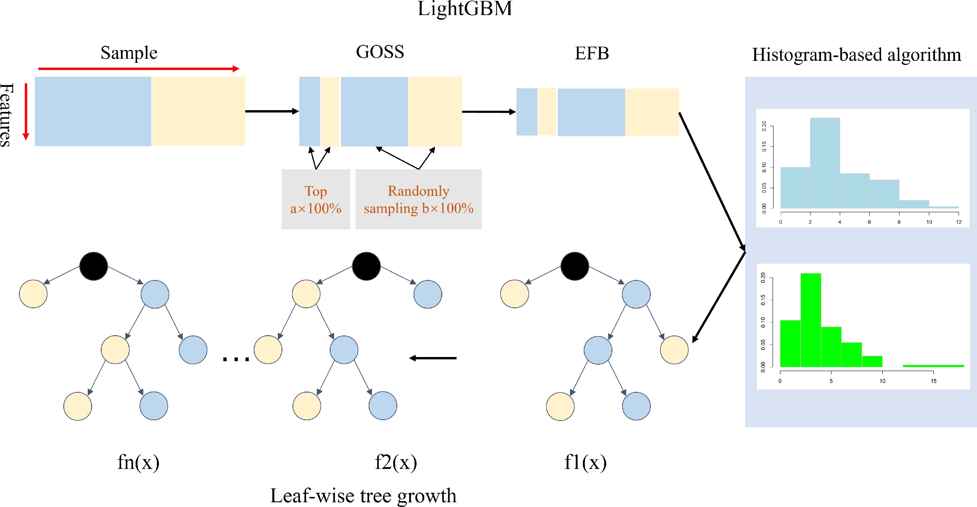
Figure 3. 

An overview of LightGBM^[57]. LightGBM includes the GOSS, EFB, histogram-based feature selection, and leaf-wise tree growth of the decision tree.

In this method, the training results are sorted in descending order based on the gradient. The top A data instances are retained as data subset a, and the remaining data are randomly sampled to yield subset b; the new training dataset consists of subsets a and b (Fig. 3). An exclusive feature bundling algorithm was proposed to decrease the number of features by bundling exclusive features into a single feature as a sparse feature matrix. In addition, unlike other boost models, a leaf-wise decision tree growth strategy is employed to split the nodes, resulting in less loss than the level-wise algorithm. Finally, it is easier to perform multi-threaded optimization and control the complexity of the dataset using the lightGBM model. Yan et al. proposed using lightGBM for F1 prediction for GS^[60]. The authors demonstrated that lightGBM had higher accuracy than XGBoost, CatBoost, and rrBLUP when the training dataset excluded parental information. However, the accuracy of lightGBM was lower than that of rrBLUP when parental information was added to the training dataset. Nonetheless, the accuracy of the lightGBM model could be affected by the population structure and kinship of the training population. Additionally, lightGBM takes less time and uses less memory than XGBoost, CatBoost, and rrBLUP.

Deep learning (DL)

Deep learning (DL), a popular research direction in artificial intelligence (AI), has developed rapidly in recent years. A series of excellent models for computer vision have been produced using DL, including multilayer perceptron (MLP), convolutional neural networks (CNN), and recurrent neural networks (RNN). Therefore, some attempts have been made to apply DL to biology to enhance GS and other techniques^[61]. Here, we focus on MLP and CNN algorithms.

MLP is a deep neural network mechanism and technology. The simplest MLP is a neural network with a three-layered structure containing an input layer, a hidden layer, and an output layer (Fig. 4)^[62]. Multiple hidden layers can be added to the network. The mathematical expressions are as follows:

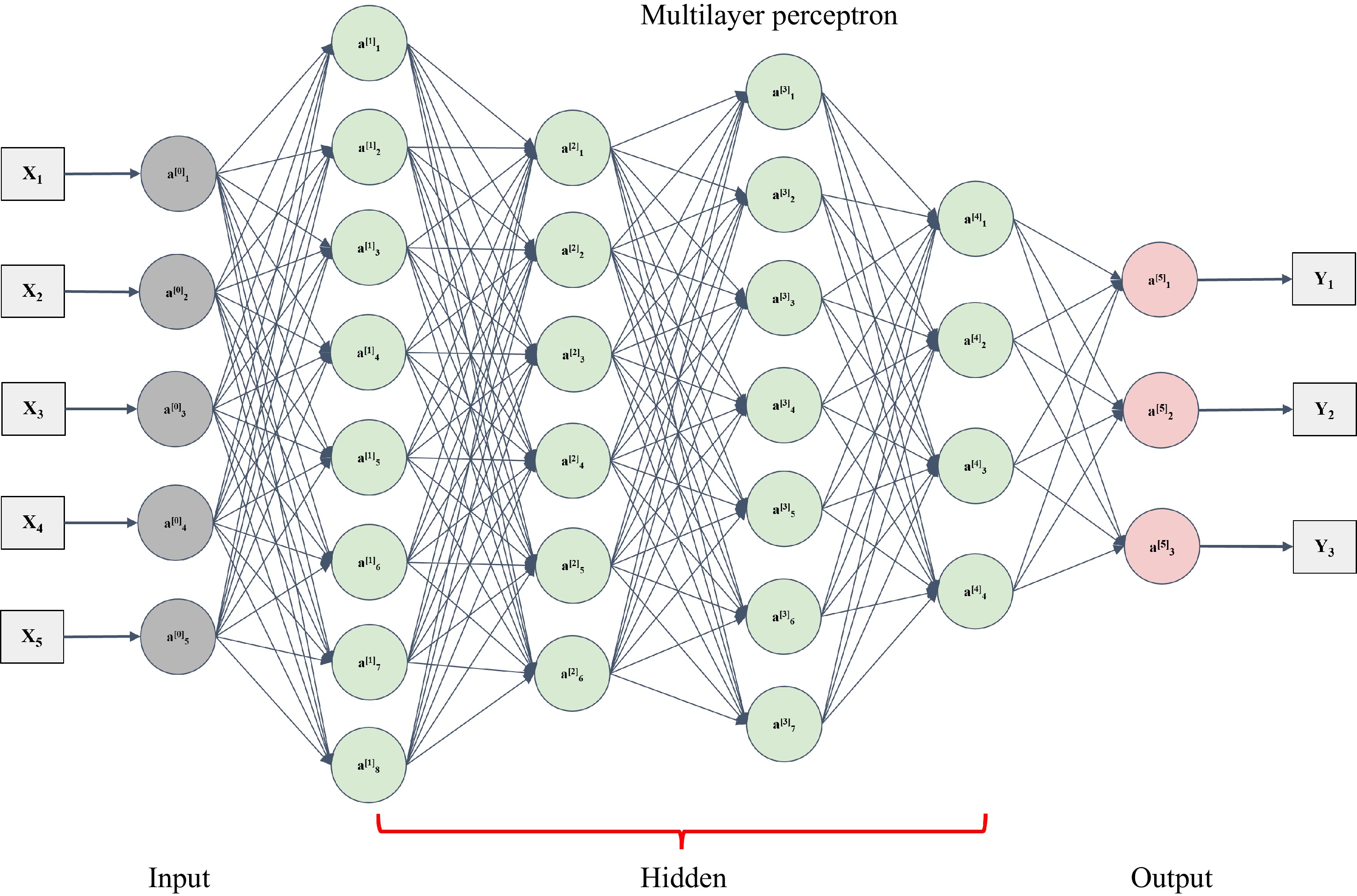
Figure 4. 

An architecture of multilayer perceptron^[62]. The multilayer perceptron includes one layer (a0 layer) with respect to input data and one layer (a5 layer) with respect to the output. The hidden layer could consist of many layers (from a1 to a4).

Here, $ X $ is the $ n\ \times\ o $ matrix for the feature, $ {W}^{1} $ is the $ o\ \times\ p $ matrix for the trained parameters, $ {H}^{1} $ is the $ n\ \times\ p $ matrix for the first hidden layer, $ {b}^{1} $ is the $ 1\ \times\ p $ vector for the bias parameters, $ {W}^{2} $ is the $ p\ \times\ m $ matrix for the training parameters, $ O $ is the $ n\ \times\ m $ matrix for the output variables, $ {b}^{2} $ is the $ \text{1 ×}\ m $ vector for bias variables, and $ \sigma $ is the activation function. All parameters can be optimized via forward propagation and backpropagation according to the loss function. Bellot et al. used MLP to predict complex human traits and determined that one hidden layer is better than multiple hidden layers^[62]. Nevertheless, another report indicates that the optimal number of hidden layers depends on the dataset^[63,64]. In general, no more than three hidden layers are normally required in GS projects^[65].

CNN plays a crucial role in DL. The predecessors of this tool date back to 1980^[66]. Nevertheless, the first formal CNN construction model, which was proposed by LeCun et al. in 1998, contains three types of layers: convolutional layers, pooling layers, and a fully connected layer (Fig. 5)^[67]. The authors also described a complete backpropagation optimization algorithm. Obtaining a convolutional kernel from convolutional layers, which focuses only on local features, is a critical step for CNN. The size of the convolution kernel determines the scope of view. The convolution of the kernel and the corresponding areas could be computed as the inner product using the equation $ \left(f \times g\right)\left(t\right)={\int }_{-\infty }^{+\infty }f\left(\tau \right)g\left(t-\tau \right)d\left(\tau \right) $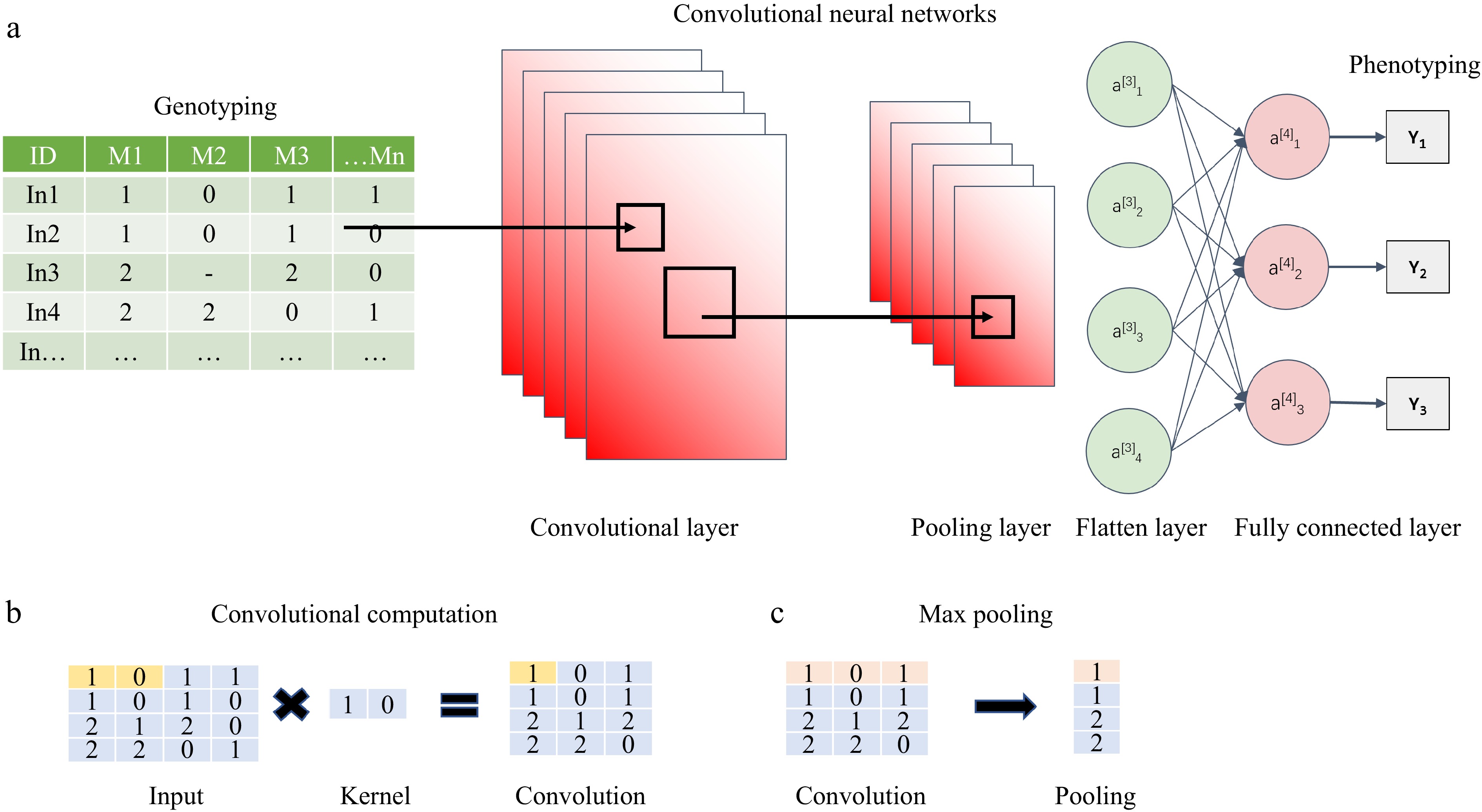. Pooling layers are periodically inserted between successive convolutional layers. The function gradually reduces the spatial size and decreases the features to reduce the need for computing resources by downsampling without affecting the results. A max-value algorithm is usually used to implement downsampling.

Figure 5. 

An architecture of convolutional neural networks^[67]. (a) General CNN algorithm, including convolutional layer, pooling layer, and fully connected layer. (b) Explanation of the convolutional computation. (c) Max pooling method.

The kernel could be set to different dimensions based on circumstances: 1D, 2D, or 3D, all of which are expressed as a weight parameter matrix to be trained in the CNN. A 1D convolutional kernel could be applied for the SNP feature, as the genotyping of each individual is expressed as a 1D vector based on previous studies, such as DeepGS^[68], DLGWAS^[69], and DNNGP^[70]. While all these models aim to enhance genomic prediction, they exhibit significant differences in their architectural designs and methodologies. DeepGS and DLGWAS both employ CNN structures; however, DLGWAS introduces a dual-stream design that significantly enhances the flexibility of feature processing. In contrast, DNNGP adopts a more conventional approach focused on efficient feature extraction, which may limit its capacity to capture complex data relationships due to its relatively simpler architecture. Meanwhile, there is a new focus on 2D expression, which remains to be tested. The convolutional layer performs dimensionality reduction. An activation function is then used to implement a non-linear approach. All these models are MLP or CNN models that do not use many layers. Nevertheless, these DL models that use convolutional layers were not shown to be more accurate than traditional models based on previous results^[64].

Comparison of ML-based GS algorithms and statistical algorithms

ML algorithms have been extensively applied to various large and high-dimensional datasets. These algorithms not only allow for the inclusion of numerous markers from high-throughput sequencing but are also suitable for different types of omics data, such as gene expression data, and functional annotation of proteins. ML models also provide important results, facilitating the identification of markers with the most significant effects on the trait of interest^[60]. Therefore, ML is highly flexible for feature processing. The biological process from gene to phenotype is highly complex, including transcription, translation, and gene networks. Traditional linear models cannot accurately capture all of these complex relationships. In contrast, many ML methods can recognize non-linear relationships between genetic markers and phenotypes, offering improved modeling capabilities^[40]. However, ML algorithms, such as DL models, require significant computational resources and large training datasets due to the many parameters to be estimated among the potential factors^[70]. Additionally, ML models, particularly DL architectures, are often black boxes, making it challenging to interpret marker effects or to understand the biological mechanisms underlying the resulting predictions. It is essential to select the appropriate ML method based on the specific characteristics of the dataset and the objectives of the GS. In general, ML model tuning should be performed to evaluate the performance and suitability of each method for a particular trait and dataset (Table 1).

Maize DH lines can be produced in a high-throughput manner in the laboratory, greenhouse, or winter nursery via yearly management. However, it is challenging to screen and develop DHs. It is not feasible to plant all DHs in the field due to the excessive workload and low-efficiency selection process. Consequently, GS is a critical step for methods involving DH^[71]. Similarly, numerous F2/F3 or BC1/BC2 materials of maize, rice, and wheat are generated on a large scale during breeding, although the genotypes of these materials are not stable and some loci are segregating. However, phenotypic prediction of these materials still increases the efficiency of the breeding process^[72,73].

Hybrid prediction

With the hybrid materials of maize or rice in place, breeders can use this model to predict the performance of different hybrid combinations^[60]. The genomic information from the selected parental lines is used to estimate the expected performance of the hybrid progeny for the target traits. These predictions help breeders make informed decisions about which hybrid combinations are likely to display superior performance and should be advanced in the breeding program.

Prediction of simulated progenies of parental lines

During inbred line selection, the two parental lines from maize, rice, or wheat must be selected to perform a single cross. A general rule is that the two parents will generate lines that have improved versions of their phenotypic traits. However, parents that have complementary advantaged genetic backgrounds tend to produce superior progeny. As a result, it is difficult to decide which combination is best when many parental lines are available. In modern breeding, each elite line could be genotyped using high-density markers, and a breeding population containing 300–400 individuals could be simulated by the genetic algorithm based on the markers of the parental lines. Each phenotypic trait of these individuals could be predicted by the trained models^[74,75]. A predicted phenotypic value could be obtained for each possible combination from two parental lines. All combinations could then be compared to facilitate decision-making based on the predicted breeding values.

The prediction accuracy for various traits is relatively variable across BLUP estimation models, Bayesian estimation models, and ML^[76,77]. The genomic estimated breeding value from GBLUP of the realized (additive) relationship matrix is equivalent to that from the marker-based rrBLUP strategy^[22,78]. Additionally, PBLUP is less accurate than GBLUP in most situations, as GBLUP can capture the effects from both within- and between-family genetic variation^[79]. There is a growing number of prior distributions and hypotheses based on Bayesian regression models, with varying levels of accuracy: the accuracy is higher when the genetic architecture of the traits complies with the prior distribution^[80].

There is a dialectical relationship between GS models and QTLs. For example, BayesB is more accurate when traits are controlled by many genes or major QTLs^[5]. Meher et al. reported that the Bayesian alphabet model is better when the traits are controlled by a few genes/QTLs with relatively large effects. To assess this issue in more detail, we used a dataset of 487 wheat individuals with 30,548 markers. The dataset included various types of wheat such as cultivars, landraces, and synthetic hexaploids, and we analyzed several models, including rrBLUP, BRR, BL, BayesA, BayesB, MLP, and CNN (Fig. 6). In some traits, BayesA and BayesB had more accurate predictions than other models when the traits were determined by multiple small-effect QTLs and a few large-effect QTLs^[80] (Fig. 6a). However, for some complex traits such as yield, the BayesA and BayesB are not always better (Fig. 6b).

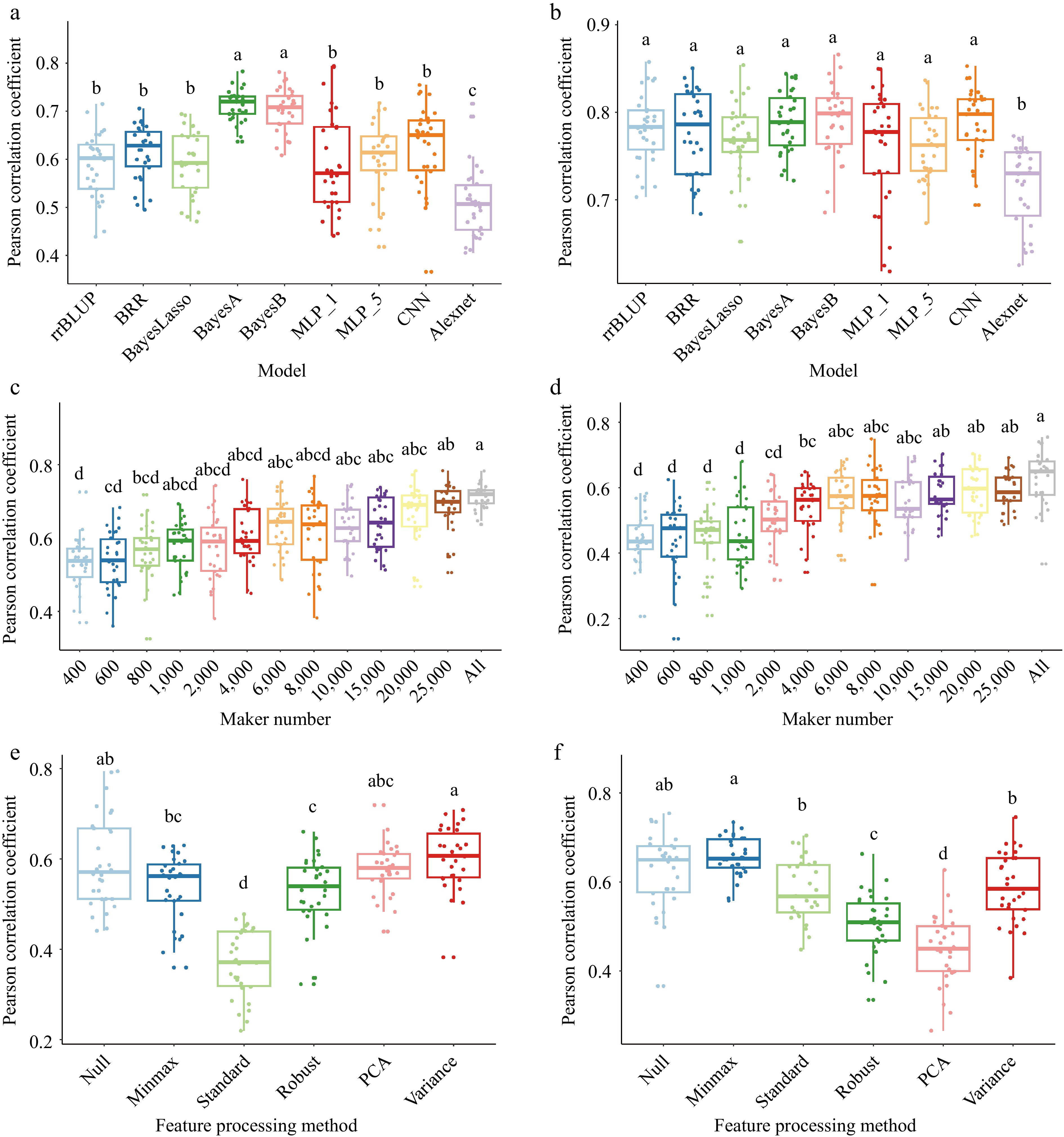
Figure 6. 

Comparison of factors on GS models prediction ability. (a) and (b) comparison of nine GS algorithms on wheat based on the Pearson correlation coefficient of the model prediction ability. (a) Plant height with two major QTLs and heritability is 75.7% in 2014 and 76.5% in 2015, (b) yield with five major QTLs and heritability is 70.1% in 2014 and 85.6% in 2015. 'MLP_1' and 'MLP_5' denote the one and five hidden layers in multilayer perceptron algorithm; 'CNN' means the one convolutional layer, one pooling layer, one fully connected layer; 'Alexnet' is based on the Alexnet architecture model. (c) and (d) Impact of marker numbers on prediction accuracy. (c) Thirteen ways of markers set were randomly selected from 30548 markers to validate the prediction accuracy through the BayesA model. (d) Thirteen ways of markers set were randomly selected from 30548 markers to validate the prediction accuracy through the MLP_1 (multilayer perceptron algorithm with one hidden layer) model. (e) and (f) Impact of feature processing on prediction accuracy. (e) Six ways of feature processing were used to validate the prediction accuracy through the MLP_1 model. (f) Six ways of feature processing were used to validate the prediction accuracy through the CNN model. 'Null' is all markers; 'minmax' is min-max scaling; 'standard' is z-score normalization; 'robust' is robust feature processing; 'PCA' is principal component analysis; 'variance' is the variance scaling. Validation of all models is conducted by five-fold cross validation and repeat 30 times. The least significant difference (LSD) is used as the significance test with threshold of 0.05.

Additionally, during the construction of models for use in GS, data preprocessing has a critical effect on the accuracy of prediction. An appropriate data preprocessing technique pipeline could help ensure the integrity and usefulness of the data, resulting in improved accuracy for GS. This preprocessing could include steps such as screening and imputation of genotyping data and filtering out missing phenotypic data and outliers^[81].

The heritability of traits is critical for prediction accuracy as well. There is a close relationship between predictability and heritability. Bayesian regression models are more accurate than BLUP regression for traits with high heritability (Fig. 6a & b), whereas traits with lower heritability should be predicted using BLUP regression models^[82]. However, if the heritability of traits is lower, the prediction accuracy can be overestimated. Consequently, GS for traits with low heritability is still quite challenging.

The size of the training population is a crucial factor for model accuracy. In general, the larger the population, the greater the prediction accuracy, but this association weakens after a certain threshold^[60,70]. Therefore, the cost of the experiment and prediction accuracy must be balanced. A representative training population of sufficient size could lead to better generalization of a model. Higher accuracy is obtained when there is a very close relationship between the training dataset and the testing dataset, such as when both are part of the same full-sib family. Insufficient or biased training data can result in poor accuracy for GS.

Genotyping provides genetic information in the form of markers or variants, which are linked with the gene of interest and can be used as features in GS models. Theoretically, the prediction accuracy depends on the number of markers used (Fig. 6c & d). Additionally, incorporating genetic features derived from genotyping into the modeling process could potentially improve the prediction accuracy for GS^[83], such as PCA, Min-Max Normalization, or others (Fig. 6e & f). However, strategies used for feature processing must be chosen carefully, as their effects on prediction ability are not always as expected (Fig. 6e & f). In practice, markers cannot explain all genetic variation; a haplotype block feature strategy could be a suitable way to explain some portion of additional genetic variation^[84]. Consequently, combining different genetic features could improve the accuracy of a model.

In previous sections, we summarized GS using models based on statistical analysis or ML. Much effort has focused on improving the prediction accuracy of all these models; however, breeding traits, especially yield, are highly complex due to the control exerted by gene regulatory networks, and innovative new models must be developed. What is the future direction of GS algorithms?

With the continuous improvement of commercial breeding systems, the types of breeding populations have become increasingly diverse, including many DHs from bi-parental populations and sets of breeding populations or lines derived from different stages of self-crosses in breeding programs and hybrid trials across multiple locations and over multiple years^[85,86]. Multi-population joint prediction models are urgently needed to address this issue. With the development of high-throughput sequencing techniques and advances in biotechnology, the cost of processing single samples has decreased, making the production of multi-omics data, including genomics^[87], transcriptomics^[88], and proteomics^[89] data easier and more convenient. The construction and preprocessing of large-scale multi-omics datasets, including screening, filtering, and integration, are challenging using traditional methods^[90,91]. With the continued collection, accumulation, and analysis of envirotypic data, enviromics is increasingly being used to explore genotype-by-environment interactions based on spatial and temporal variability at multidimensional scales^[85,92]. This analysis provides insights into the environmental drivers of the distribution of elite germplasm, facilitates the screening of breeding materials, and enhances the precise evaluation of plant varieties, ultimately leading to advanced breeding processes.

Complex quantitative traits, such as yield, are regulated by multiple genes and their interactions. These traits pose significant challenges for current predictive models due to their genetic complexity. Each gene contributes a small effect to the overall phenotype, and these effects accumulate to determine the final trait expression. Consequently, to capture interactions between genetic factors and specific environments, much more novel and innovative models must be explored. Three specific models for genomic selection (GS) based on CNN architecture have been reported: DeepGS^[68], DLGWAS^[69], and DNNGP^[70]. These methods have proven to be competitive with others and outperform traditional methods in some respects due to their ability to handle high-dimensional data. We believe that AI holds tremendous potential applications for GS. Some researchers have started to use RNA-seq data to enhance the efficiency of selection by integrating gene expression data into GS models using kernel-based methods, which have been used to capture complex genetic interactions and non-linear relationships between genetic variants and phenotypic traits in animals^[93].

However, applying these models directly for GS might not be straightforward, since they are primarily designed for computer vision (CV), speech recognition, and natural language processing (NLP), especially Bidirectional Encoder Representations from Transformers (BERT)^[94] and Generative Pre-trained Transformer (GPT) based on transformer architecture models. Genomic data are different from text data, making it necessary to preprocess and represent the genomic sequences in a format suitable for the models. This may involve encoding variants, genomic regions, or other relevant genetic features appropriately^[70,83]. Directly applying ML models is not better than Bayesian models and rrBLUP, like AlexNet, is not very well suited for GS applications^[63] (Fig. 6a & b). It is important to handle the sequential nature of genetic data and to ensure that the representations capture the relevant information.

Other technologies for applying these models to GS could also be considered: the underlying transformer architecture and the transfer learning principles they employ could be adapted for GS with the appropriate modifications. DeepCCR^[95] improves contextual comprehension by integrating BiLSTM layers, which are particularly beneficial for the interpretation of sequential data. In comparison, SoyDNGP^[96] employs a three-dimensional input matrix, enabling it to capture intricate genotypic variations and provide richer feature density than the one-dimensional vectors used in other models. GPformer^[97] utilizes innovative attention mechanisms to enhance the representation of SNP relationships, thereby enhancing predictive accuracy. Meanwhile, Dual-Extraction Modeling (DEM)^[98] stands out with its dual-extraction mechanism, effectively integrating multi-omics data and improving performance through noise reduction and enhanced feature separability. Collectively, the advancements exemplified by GPformer, SoyDNGP, and DEM reflect a trend toward developing more complex and integrated processing architectures that effectively address the multifaceted challenges of genomic prediction. Pre-training the models on large-scale genomic data or related tasks could be beneficial for adapting the pre-training process to GS, capturing meaningful patterns from the pre-training data, and assisting in downstream GS tasks. After pre-training, it is essential to fine-tune the models for specific GS tasks. The fine-tuning process helps adapt the models to specific tasks, and the relationships between genetic variants and performance can be deduced by incorporating domain-specific knowledge into the models. This could be achieved by incorporating prior knowledge about the biology and genetic pathways of the organism, or by using specialized loss functions that account for the specific requirements of GS^[92].

Breeding 4.0 reflects the future ability to combine any known alleles into optimal combinations, potentially revolutionizing the field. This stage of agriculture will rely on the development of highly advanced genetic manipulation technologies that can be used to obtain ideal genetic combinations for specific traits. In future breeding pipelines, large-scale multimodal data will be created and developed, such as DNA/protein sequences; text annotation of multi-omics data; images, audio files, and video files from phenomic analysis; sensor readings; and telemetry data^[99]. Additionally, numerous public databases, data-sharing platforms, and research papers will be channeled into the pipelines. We believe that GS can serve as a bridge from AI to Breeding 4.0 with innovations in ML, NLP, CV, and other novel technologies. Such enhancements will extend the use of AI in breeding programs.

In summary, the above factors could enhance the prediction accuracy of GS models. These advanced analytical methods can handle big genomic data, identify complex patterns, and enhance prediction accuracy. As computational tools continue to improve, they could enhance the efficiency and effectiveness of genomic prediction models. By considering a wider range of molecular information, researchers can gain a deeper understanding of the biological mechanisms underlying traits and develop more accurate prediction models for GS.

Many innovative models based on ML are applied to GS to improve the efficiency of breeding. However, not all ML methods significantly enhance prediction accuracy compared to traditional methods, such as BLUP estimation and Bayesian estimation. All of these methods are useful under the appropriate scenarios, and there is currently no unified strategy for GS. Consequently, all types of models for enhancing the accuracy of GS should be considered on a case-by-case basis based on previous studies (Table 2, Fig. 6a & b). Compared to ML, the development of GS models is in its early stages, but GS will serve as a tool for enhancing breeding programs. AI technologies can analyze vast repositories of breeding data, scientific literature, and expert knowledge to discover new patterns, relationships, and insights. These findings can be shared and transferred to breeders, scientists, and stakeholders, fostering collaboration, innovation, and accelerated progress in the breeding community. AI will play a crucial role in accelerating the transition to Breeding 4.0 by facilitating the creation of large-scale multimodal datasets, complex predictive modeling, and precise decision-making processes in crop breeding programs.