A WPT system with DDQ pads and LCC compensation topology for improving high misalignment tolerance and interoperability in the Y direction

Today, people's increasing attention to environmental pollution, energy consumption, and rising oil prices has driven interest in electric vehicles (EVs) as a sustainable transportation solution^[1]. The wireless charging of electric vehicles provides several advantages for electric transportation^[2,3]. This innovative technology significantly improves the convenience for users to charge electric vehicles and reduces reliance on physical charging connections^[4−7].

In wireless power transmission technology^[8], misalignment between the transmitting and receiving ends of magnetic coupling structures is inevitable, which can lead to a decrease in the coupling coefficient and a decrease in system transmission capacity. In order to solve the problem of poor misalignment tolerance in the coupling zero-crossing direction of DD coils, scholars have proposed dual receiving coils such as DDQ coils and BP coils^[9]. For the two types of coils mentioned above, the DD and Q coils should be decoupled from each other, and the BP coil also needs to overlap with each other to achieve mutual decoupling and avoid introducing cross-coupled reactive power. This requires special design of magnetic coupling structures, which puts forward requirements for design freedom and is not conducive to the application and promotion of multiple receiving coils. Interoperability in wireless power transmission technology refers to the ability of the receiving coil to adapt to different shapes of the receiving coil, in order to accommodate the coil designs of charging stations and rechargeable batteries from different manufacturers.

Some scholars use special algorithms or control methods^[10−12] to solve the problem of low misalignment tolerance of coils. However, both of these methods are too complex, requiring redesign of parameters and schemes for different sizes and forms of this coupling structure, resulting in low universality and adaptability. The proposed method provides a passive decoupling principle for multi-coil systems. Its applicability depends on whether the mutual inductance matrix of the secondary coils can be compensated by a realizable passive decoupling network at the operating frequency.

Some scholars also adopt variable topology structures to implement topology switching in different coupling states^[13], so that magnetic structures with higher coupling states are working. But this approach requires additional switching devices, increases costs, reduces efficiency, and also requires redesign according to different magnetic structures.

Several studies^[14,15] have optimized the parameters of compensation networks to attain a high coupling coefficient while ensuring robust tolerance to coil misalignment. Nevertheless, this approach is susceptible to fluctuations in input voltage and load resistance.

To tackle the challenge of system interoperability, some researchers proposed a dual-coupled inductive power transfer (IPT) system integrated with a hybrid topology^[16,17]. This design is engineered to enhance the system's capability to deliver stable constant voltage or constant current outputs even under severe misalignment conditions. Specifically, different coupling coil sets are adaptively selected according to the misalignment distance, thereby enabling consistent output power across a broad range of spatial positions.

In addition, traditional DDQ coils have a pair of D coils wound in reverse series, and the coil current is always the same^[18]. However, due to the difference in mutual inductance between the pair of D coils and the primary side, this paper connects the pair of D coils separately to a rectifier. As the rectifier can automatically match the conduction and turn-off of the diode according to the direction of the current, it greatly improves the interoperability of the system.

In this paper, the size of the DDQ coil and LCC compensation parameters are specially designed to achieve strong misalignment tolerance and constant current output capability of the system. The article also optimized the parameters of the DDQ coil, but only for the magnetic optimization of the circular coil at the alignment position of the transmitting end^[19].

We first analyzed the T-type network model of mutual inductance and obtained the decoupling model and decoupling conditions of the DDQ coil. Then, the magnetic coupling structure was designed and optimized, and specific examples were given on how to optimize the magnetic field. Finally, a prototype was built for experimental verification.

In response to the above issues, especially the misalignment tolerance capability of the DDQ coil along the Y direction, this paper proposes a new rectifier structure for decoupling the DDQ coil, which has the following advantages:

(1) Only one bridge arm is connected in parallel after the bridge rectifier to reduce volume. The equivalent mutual inductance of this system is the sum of the absolute values of the mutual inductances. Compared with a traditional DDQ coil, it has a stronger tolerance for misalignment. The LCC compensation parameters were designed to achieve load-independent constant current output, while also reducing the variation of output current with coupling. By using a mutual inductance T-type network model, a decoupling method based on DDQ coils is obtained, which can be generalized and is applicable to multi-coil structures with no limitations on size and shape.

(2) Decoupling the secondary DDQ coil through passive components and a T-shaped equivalent model increases the design freedom of the magnetic coupling structure. For a traditional DDQ coil, only two center taps are needed to decouple the secondary coil, without introducing reactive power and improving efficiency.

(3) The DD coil of a traditional DDQ coil is wound in reverse series. If the primary side is a square coil, the DD coil will not be able to transmit energy at the aligned position. This wastes the energy transmission capability of the coil at that position. In this paper, decoupling is used to make the three coils of the DDQ coil independent of each other, making it adaptable to primary coils of different shapes, increasing its applicability, and enhancing its interoperability.

The wireless power transmission system with LCC/LCC compensation topology is shown in Fig. 1. The primary side is a traditional DD coil, and the secondary side is the DDQ coil. The three groups of coils on the secondary side are connected to three parallel half-bridge rectifier arms, where LM and CM are decoupling elements. The equivalent model of the decoupled controlled source is shown in Fig. 2.

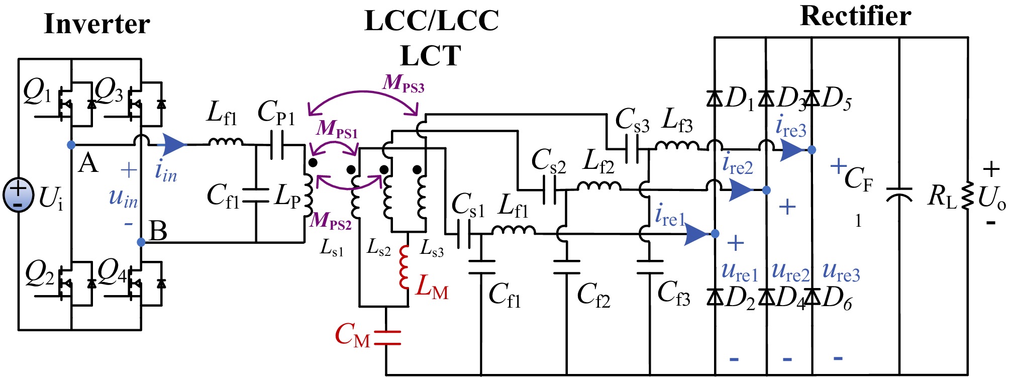
Figure 1. 

The circuit diagram of a WPT system with decoupling DDQ coils.

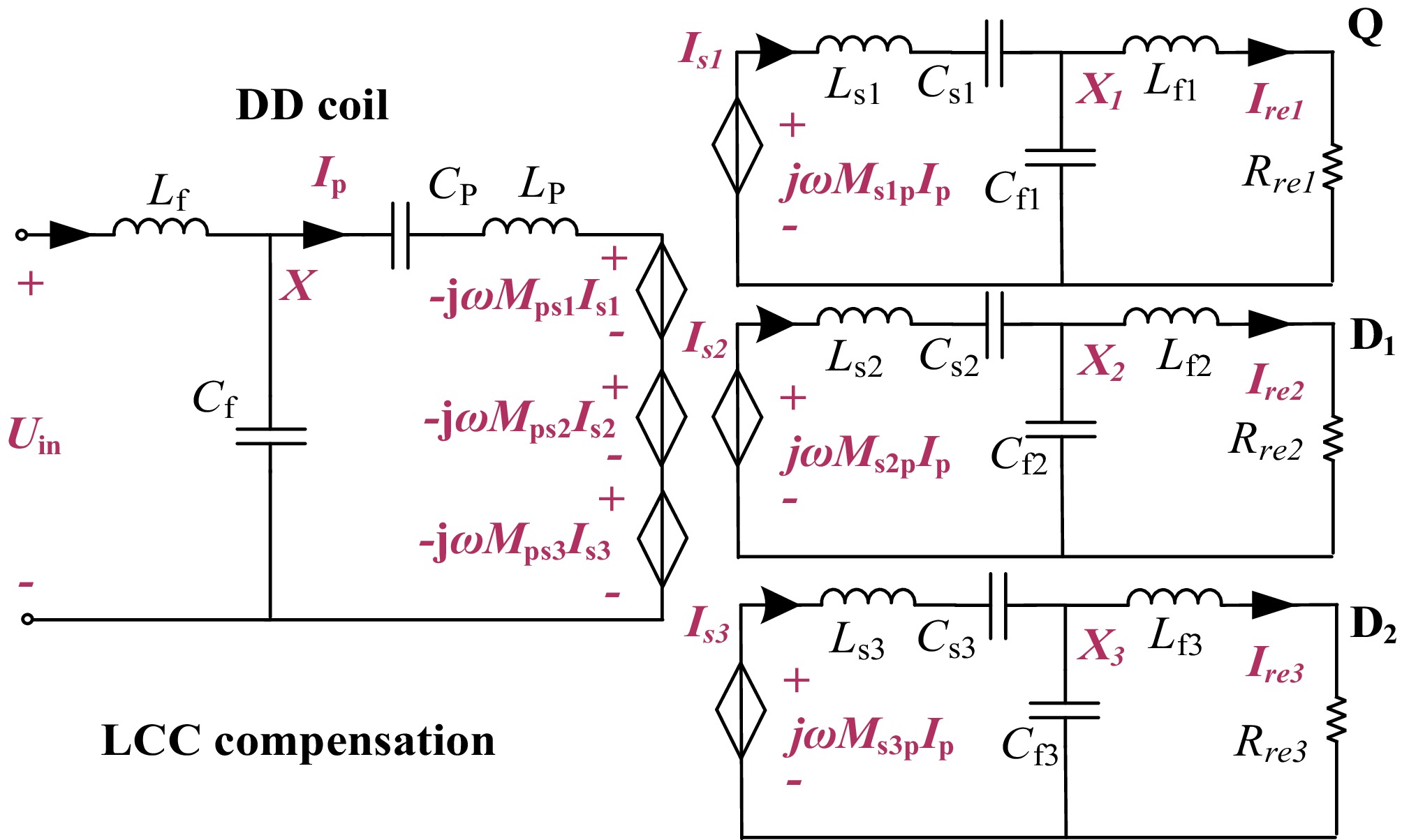
Figure 2. 

The controlled source equivalent model diagram.

According to the T-equivalent model, we can obtain the rectified input currents of each branch after decoupling the model, namely Ire1, Ire2, and Ire3 is shown in Eq. (1). Among them, X, X1, X2, and X3 are the LCC compensation bridge arm impedances of the DD coil on the primary side, the Q coil on the secondary side, and the two D coils on the secondary side, respectively.

By inputting Ip into Ire, the expressions for the currents of each branch can be obtained, as shown in Eq. (2):

Due to the fact that the rectifier is a half-bridge rectifier, the output current expression is shown in Eq. (3). From Eq. (3), it can be seen that the load output current is independent of the load, and the system has a constant current output capability.

It is worth mentioning that due to the decoupling of the three coils of the secondary DDQ coil, the equivalent mutual inductance of the primary and secondary sides is the sum of the absolute values of the mutual inductance of the primary and secondary coils, as shown in Eq. (4):

The decoupling method and compensation parameter design rules will be elaborated below. The decoupling model of the secondary DDQ coil is shown in Fig. 3. The pair of D coils are symmetrical to the Q coil; therefore M_S1S2 = M_S1S3 ≠ M_S2S3. In order to achieve capacitor decoupling, it is necessary to compensate the mutual inductance of the three coils to an equal state. As shown in Fig. 3 (I) is the equivalent model of T-type mutual inductance for the pair of D coils. The function of the decoupling inductance is to make the mutual inductance of the three coils the same, as shown in Eq. (5). By combining the two formulas in Eq. (5), it can be concluded that the function of LM is to supplement the mutual inductance between the two D coils and the Q coils. Therefore, the expression for LM is shown in Eq. (6).

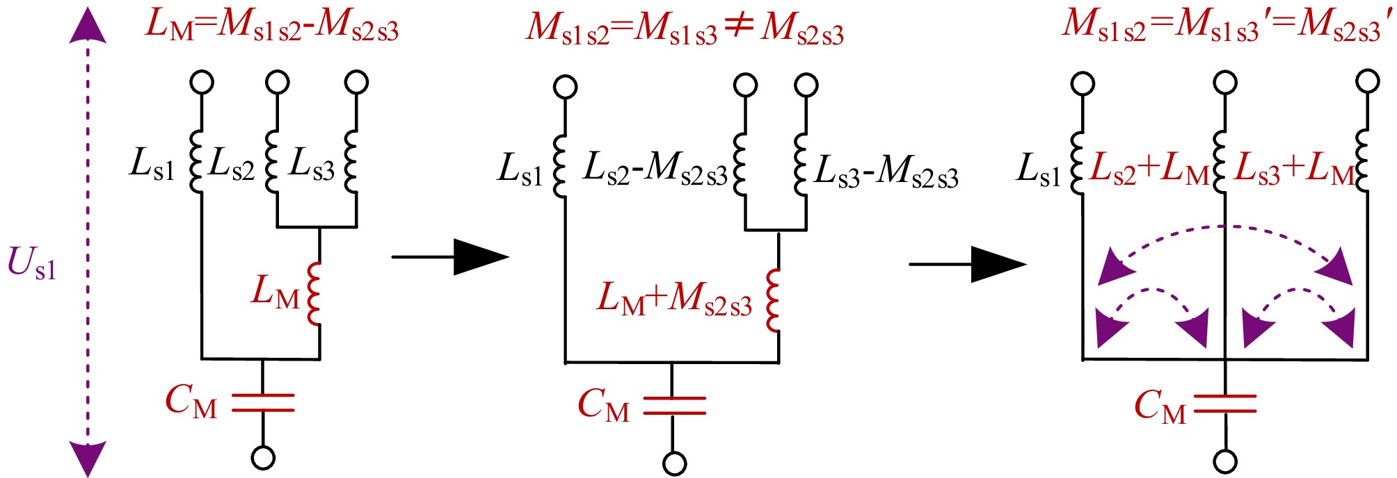
Figure 3. 

Decoupling model of a DDQ coil.

Similarly, the effect of connecting the center taps of the pair of D coils in series with LM is to make the mutual inductance MS2S3 = MS1S2. Therefore, in Fig. 3 (II), the mutual inductance of the three coils is the same, and decoupling can be achieved by compensating for the mutual inductance of the disconnected coil with decoupling capacitor CM. The expression for coil voltage is shown in Eq. (7). It was found that the two formulas in Eq. (7) are equal; therefore, the model holds true. The decoupling capacitor CM should compensate for the mutual inductance MS1S2, as shown in Eq. (8):

After decoupling the DDQ coil, the design rules for the LCC compensation topology, as shown in Eq. (9), are provided:

This method introduces a decoupling inductance LM and compensates for the mutual inductance to make the mutual inductance of the secondary coils Ls2 and Ls3 equal to Ms1s2, so that the mutual inductance of the three groups of secondary coils is the same. Then, through a T-shaped decoupling model, the three groups of coils are decoupled from each other. The applicable conditions for this method are: Ms1s2 = Ms1s3 ≠ Ms2s3. From the above analysis, it can be concluded that the decoupling condition is only related to the mutual inductance relationship between the coils. Therefore, for a general multi-coil secondary structure, the decoupling condition can be written in a simple pairwise form. For any two secondary coils i and j, the coupling term introduced by their mutual inductance should be cancelled by the equivalent reactance provided by the decoupling network. Therefore, the required condition is X_dij + ω₀ M_ij = 0, where ω₀ = 2πf, M_ij is the mutual inductance between the i^th and j^th secondary coils, and X_dij is the equivalent decoupling reactance between these two coils at the operating frequency.

If M_ij is positive, the required negative reactance can be provided by a capacitor; if M_ij is negative, the required positive reactance can be provided by an inductor.

The decoupling DDQ magnetic coupling structure proposed in this article is shown in Fig. 4. The primary side is a traditional DD coil, and the secondary side is a DDQ coil. The three coils on the secondary side are independent of each other and do not exchange reactive power. Decoupling components are connected to the same-named end taps of the three coils.

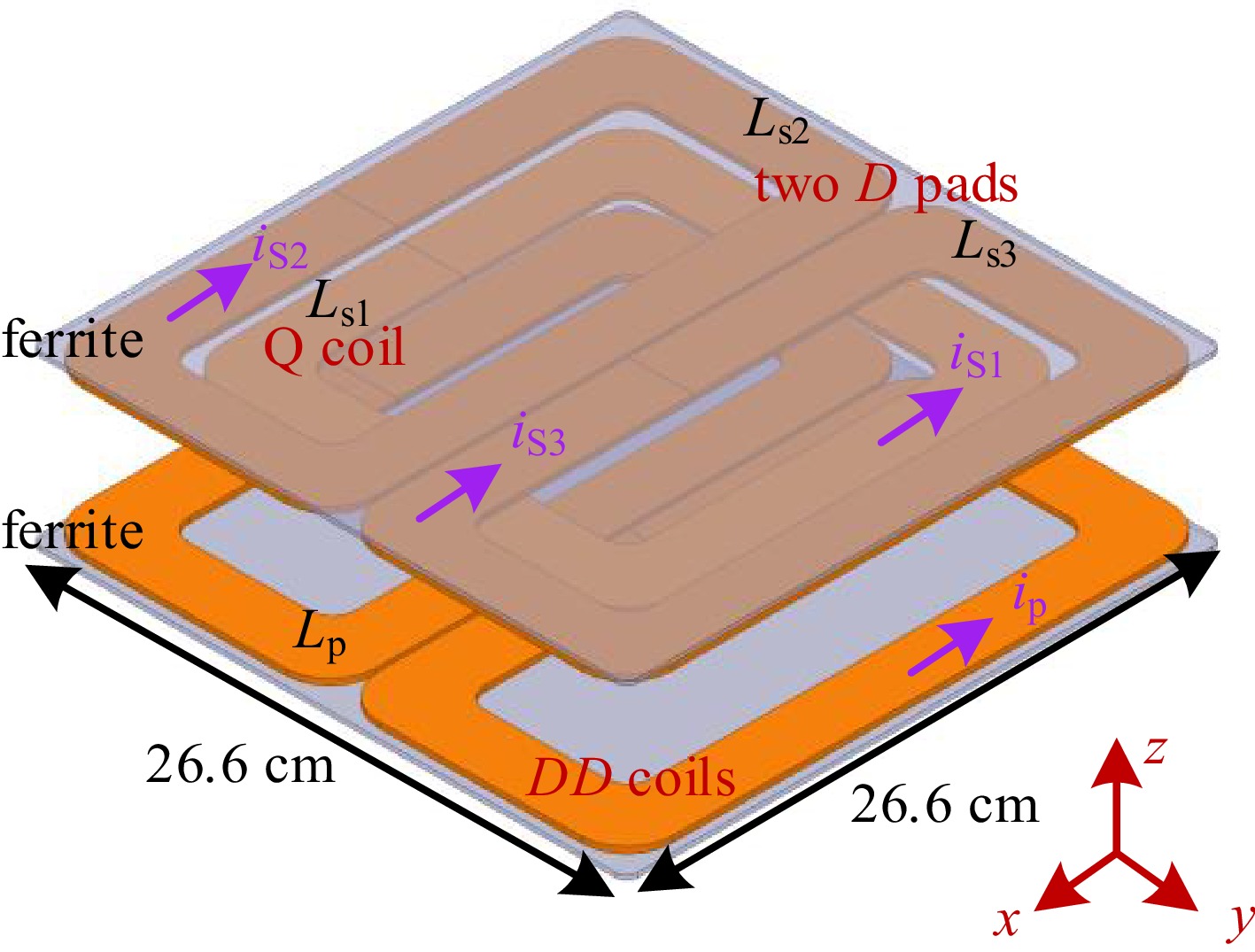
Figure 4. 

Schematic diagram of a decoupling DDQ coil.

When both the primary and secondary sides are traditional DD coils, there will be coupling zeros in the Y direction, with a small misalignment range and poor misalignment tolerance. The specific magnetic field diagram and schematic diagram are shown in Fig. 5.

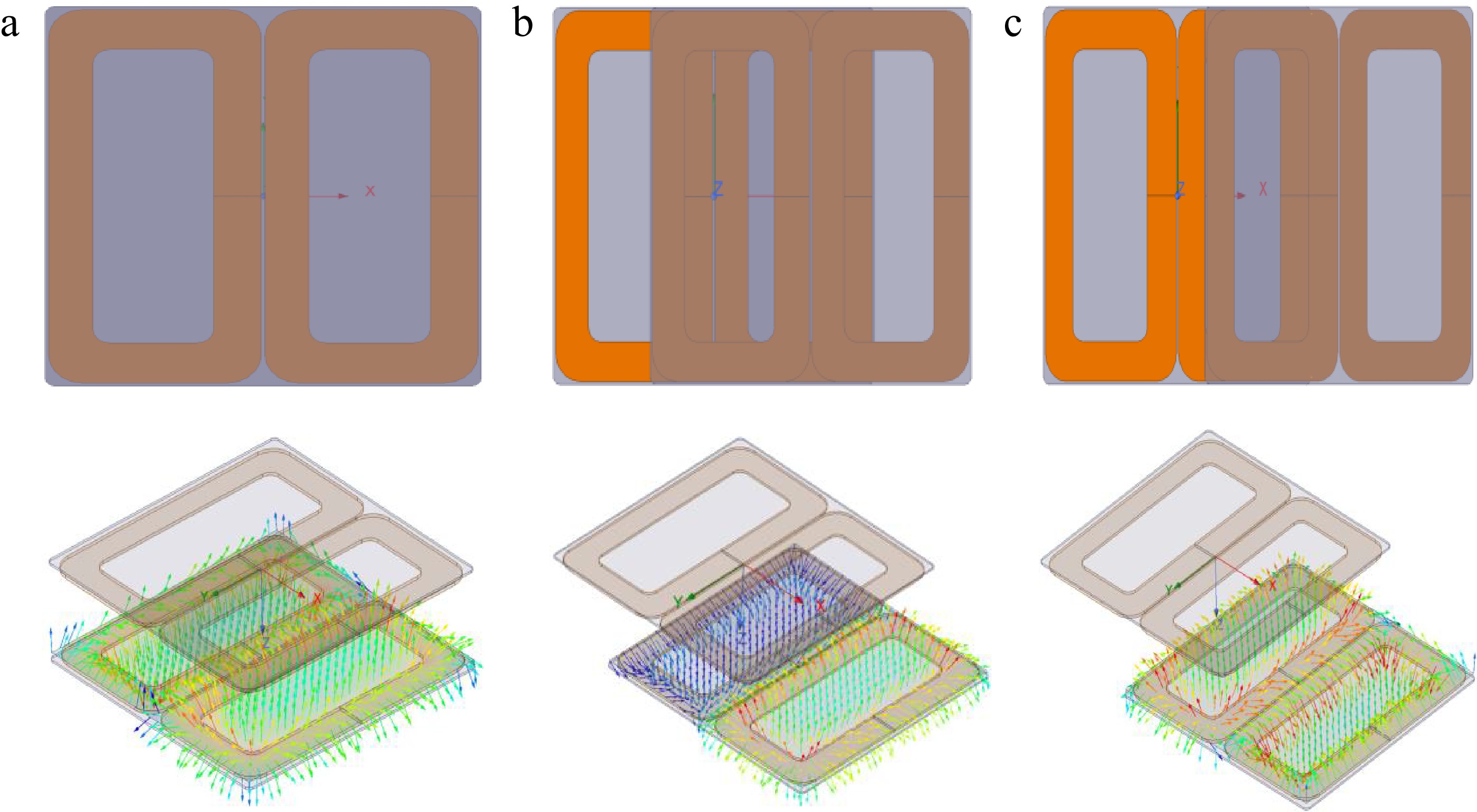
Figure 5. 

The relative position diagram when both the primary and secondary sides are DD coils and the schematic diagram of the secondary side receiving magnetic induction lines: (a) facing position, (b) misaligned 8 cm along the Y direction, (c) misaligned 12 cm along the Y direction.

From Fig. 5, it can be seen that in the facing position, the equivalent magnetic flux passing through the Q coil is zero. However, after being displaced along the Y direction by a certain distance, the equivalent magnetic flux of one of the D coils becomes zero, while the magnetic flux of the Q coil is not zero at this time. Therefore, the Q coil can supplement the coupling zero point of the DD coil. The mutual inductance variation curve misaligned along the Y direction is shown in Fig. 6.

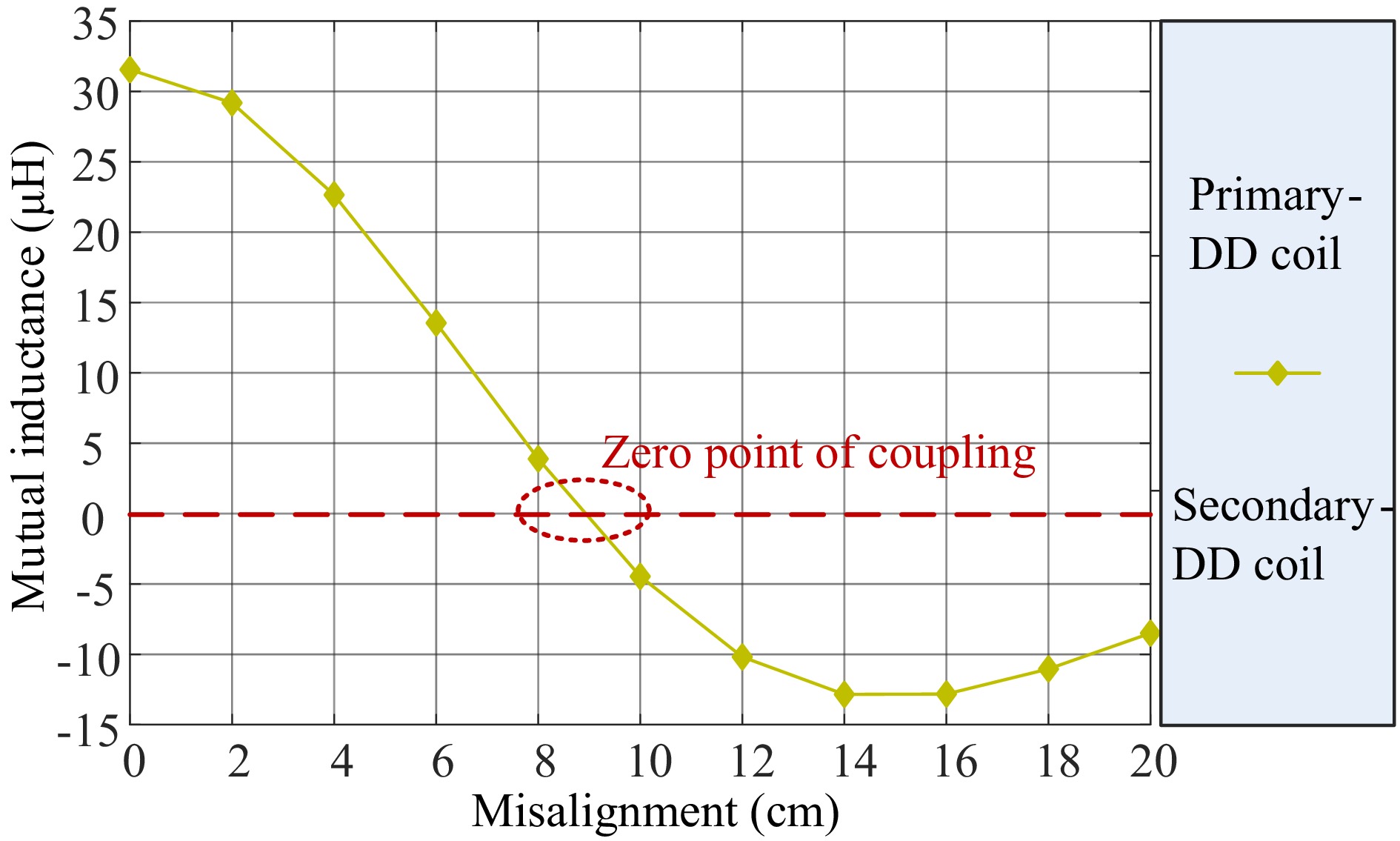
Figure 6. 

Mutual inductance curve of the DD coil misaligned along the Y direction.

When the traditional DD coil is misaligned along the Y direction, the mutual inductance rapidly decreases, and a coupling zero point appears at 8 cm, and then the mutual inductance becomes negative.

In Fig. 5, if the secondary side is a DDQ coil, it can be seen that in the facing position, the equivalent magnetic flux received by the Q coil on the secondary side is zero, while when displaced to the middle position in Fig. 5, the equivalent magnetic flux received by the Q coil is not zero. Therefore, adding the Q coil can effectively compensate for the coupling zero point of the DD coil in the Y direction. The schematic diagram of the magnetic field vector of the DDQ coil is shown in Fig. 7.

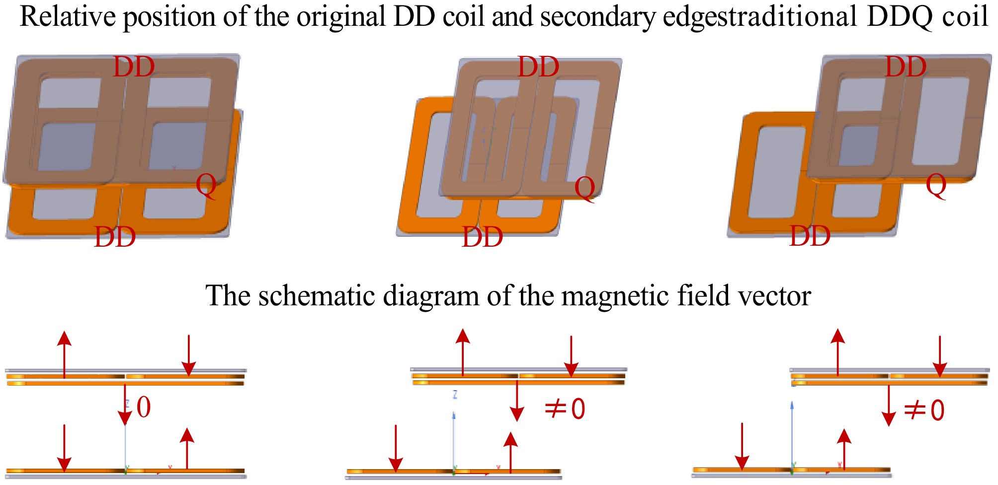
Figure 7. 

The schematic and position diagram of the magnetic field vector when the primary side is the DD coil and the secondary side is the DDQ coil displaced along the Y direction.

In Fig. 7, the process of Y-direction relative displacement of the secondary DDQ coil from the facing position is demonstrated. When in the facing position, the Q coil is decoupled from the primary DD coil, and during the misalignment process, the mutual inductance between the Q coil and the primary DD coil compensates for the mutual inductance lost by the secondary DD coil.

In order to solve the coupling zero point in the Y direction, a Q coil was added, and the two sets of coils are in parallel. In the range of facing position and small misalignment, the DD coil dominates. In the range of large misalignment and coupling zero point, the mutual inductance of the Q coil can compensate for the rapidly decreasing mutual inductance of the DD coil.

In Fig. 8, the addition of the Q coil to the DDQ coil effectively compensates for the coupling zero point when the DD coil is misaligned along the Y direction. The equivalent mutual inductance is shown in Eq. (10):

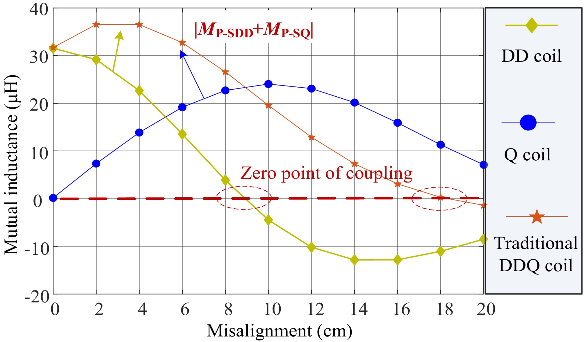
Figure 8. 

Mutual inductance curve of the DDQ coil misaligned along the Y direction.

This is a solution to the problem of reduced coupling from the perspective of supplementing mutual inductance. As we can observe from Fig. 7, when the total magnetic flux direction received by a pair of D coils on the secondary side changes, they cannot change the current direction of any D coil in the pair. If a pair of D coils can freely change their current direction according to the direction of the received magnetic flux, thereby changing the direction of the magnetic field, it can fundamentally solve the problem of rapid zero crossing of DD coil coupling. As shown in Fig. 9.

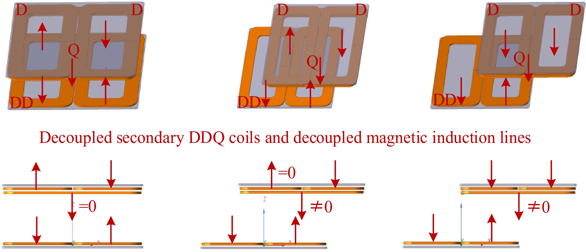
Figure 9. 

Schematic diagram of magnetic induction lines with mutual decoupling DDQ coils displaced along the Y direction.

In Fig. 9, the three coils of the secondary-side DDQ are decoupled from each other, and the current direction can be adaptively changed according to the magnetic flux received by each coil, which fundamentally solves the problem of weak misalignment tolerance of the DD coil along the Y direction.

If the DD coil and Q coil cannot be decoupled from each other, this approach will not hold, as the coupling of the two coils will introduce reactive power and reduce system efficiency. Therefore, we considered the possibility of finding a simple and effective coil decoupling method by reconstructing the magnetic field so that different coils do not affect each other, in order to increase the interoperability between coils and further increase the misalignment tolerance of coils. The solution is the coil decoupling method proposed in this paper, as shown in Figs 1 and 3.

Due to the fact that the pair of D coils in the DD coil is wound in reverse series, their current amplitudes are the same; due to the opposite winding directions, the magnetic fields generated are in opposite directions. When the primary coil is a bipolar coil similar to DD and undergoes relative misalignment, a pair of D coils will receive magnetic fields in opposite directions, and the DD coil as a whole cannot make changes to the magnetic fields in opposite directions. The decoupled DDQ coil can effectively solve this problem.

In Fig. 10, the mutual inductance variation of each coil can be obtained when the Y-axis is not aligned. It can be seen that within the misalignment range of 16 cm, the equivalent mutual inductance of the decoupled DDQ coil is higher than that of the traditional method.

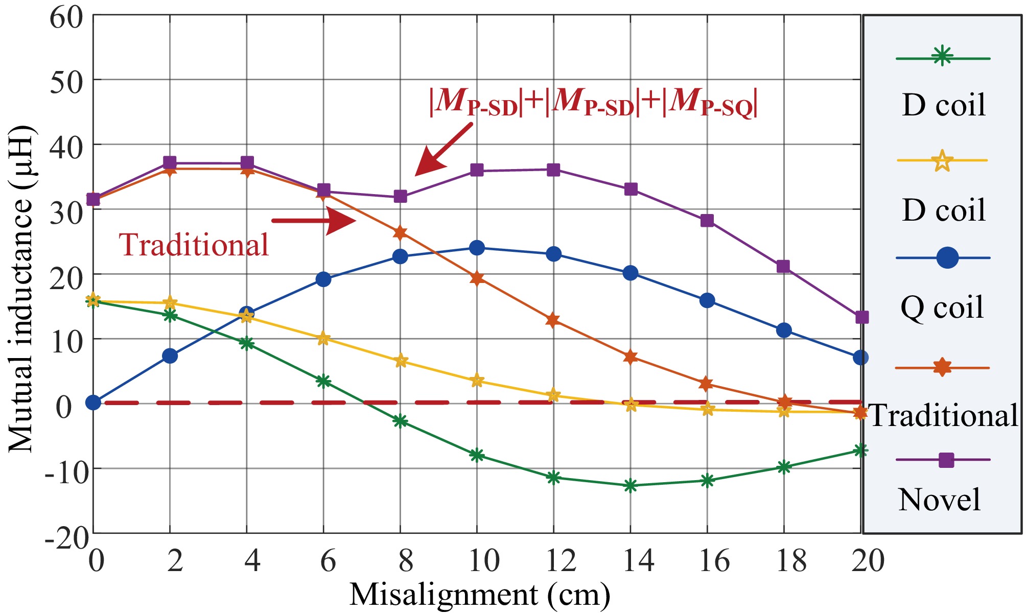
Figure 10. 

Curve of mutual inductance between a decoupling DDQ coil and a primary coil with Y-axis misalignment.

The equivalent mutual inductance of the decoupled DDQ coil is shown in Eq. (4). Compared with the equivalent mutual inductance in Eq. (10) of the traditional DDQ coil, the improved method has a higher equivalent mutual inductance, enhancing the misalignment tolerance and interoperability of the DDQ coil.

In order to optimize the improved DDQ mutual inductance curve in Fig. 10, we have decided to explore the influence of Q coil design on the mutual inductance changes when decoupling DDQ coils are misaligned along the Y direction, starting from the size and number of turns of the Q coil.

The size of the DD coil on the primary and secondary sides is exactly the same, while the size of the Q coil will affect the change in mutual inductance between the primary and secondary coils, thereby affecting the system's output and misalignment tolerance capability. Therefore, parameter scanning is performed on the size of the Q coil in finite element simulation software to obtain the optimal mutual inductance variation curve. We expect to minimize the external dimensions of the Q coil to be consistent with those of the DD coil, so we change the number of turns and internal dimensions of the coil to obtain a smoother mutual inductance curve.

We use the number of coil turns as a constraint condition, with the goal of obtaining a smoother equivalent mutual inductance curve. From Fig. 11, it can be seen that when the number of turns of the Q coil is 10, the equivalent mutual inductance of the system fluctuates greatly. Through parameter scanning, when the number of coil turns is 15, the equivalent mutual inductance of the system is large, and the variation amplitude is small. At this time, the misalignment tolerance of the magnetic coupling structure is high. The equivalent mutual inductance of the system is shown in Eq. (4), which is the sum of the absolute values of the mutual inductance between the primary coil and each secondary coil.

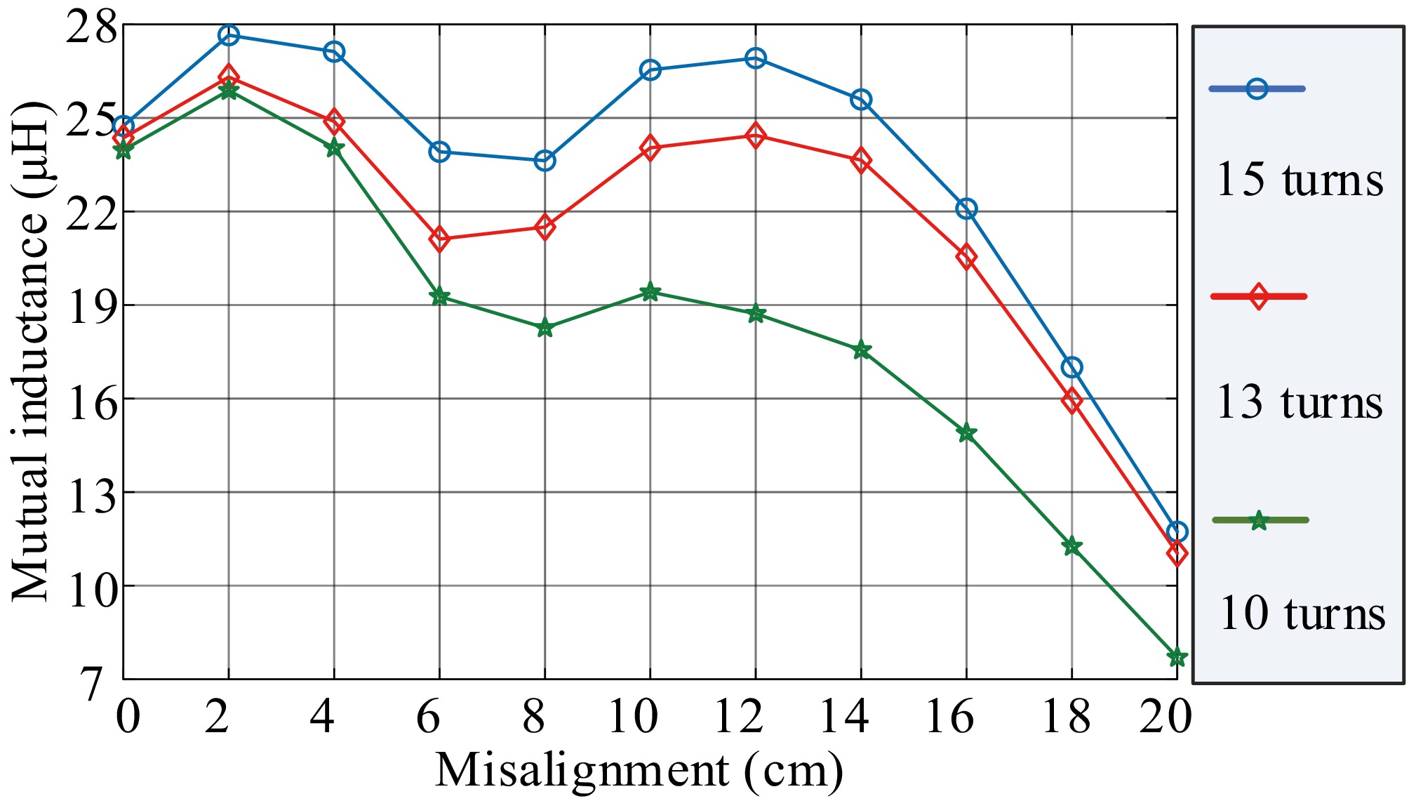
Figure 11. 

Equivalent mutual inductance of magnetic coupling structure under different turns of the Q coil.

To validate the high misalignment tolerance of the proposed structure, a 1.7 kW experimental prototype with DDQ coils and an LCC/LCC compensation topology is constructed, in which the secondary DDQ coil is split into three coils and connected to the novel rectifier, as shown in Fig. 12. The transmission distance is 7 cm. The circuit parameters are shown in Table 1.

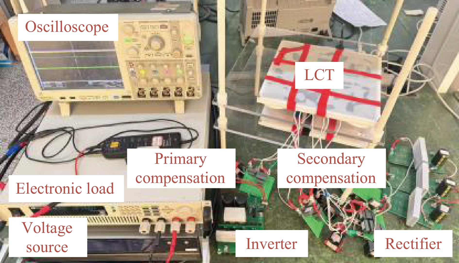
Figure 12. 

The experimental prototype.

Figure 13 shows the measured changes in mutual inductance of each coil when displaced along the Y direction. The trend of mutual inductance variation in the simulation is the same as that in Fig. 11.

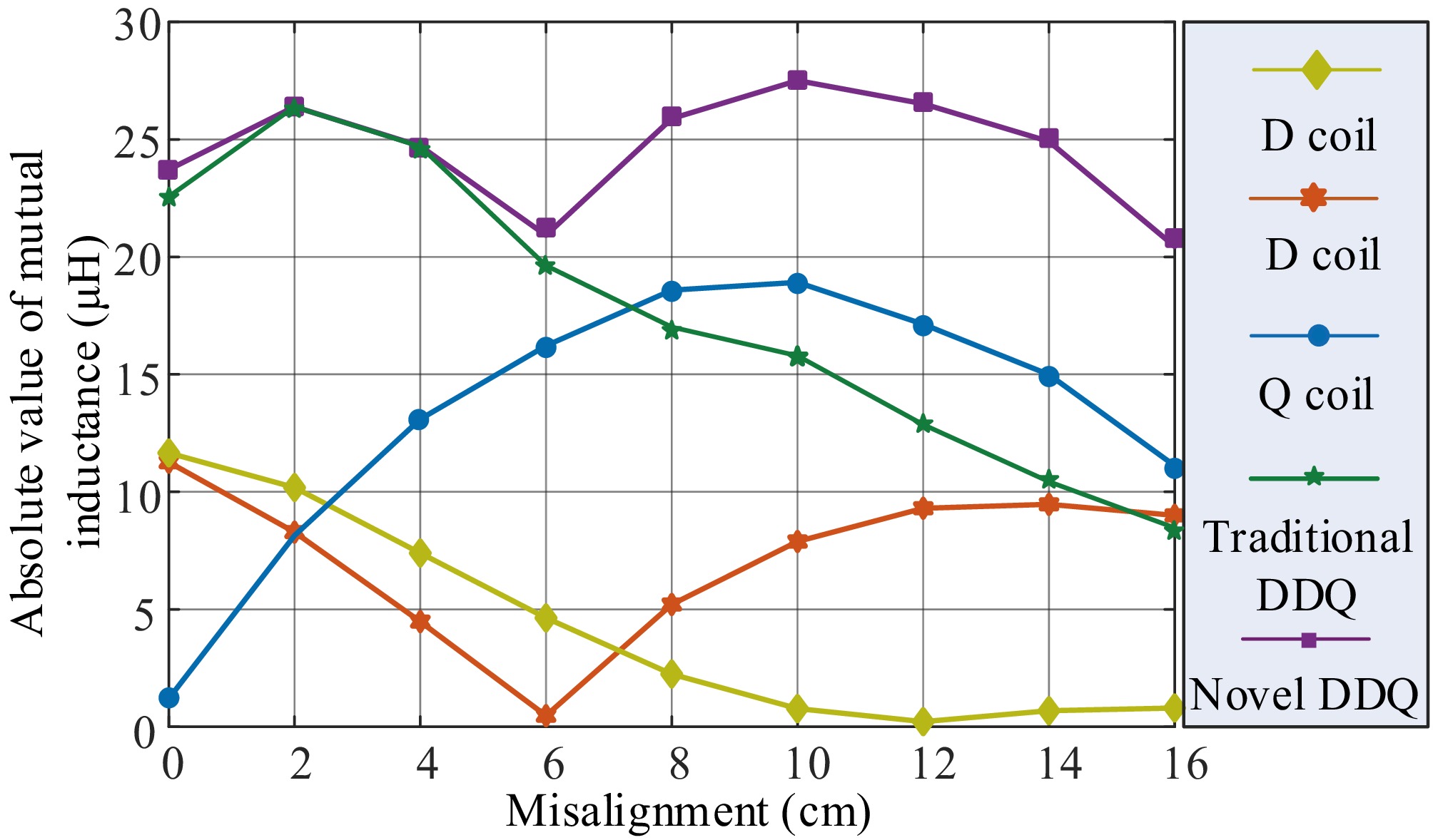
Figure 13. 

Actual measurement of coil mutual inductance.

The curves of output current and efficiency with coil misalignment are shown in Figs 14 and 15. The trend of the output current vs misalignment curve in Fig. 14 is the same as that of mutual inductance in Fig. 13, which verifies the correctness of the theoretical analysis of Eq. (4). The improved output current curve has a significant difference compared to the traditional output current curve after 8 cm, and the improved output current is significantly higher than that of the traditional method, with stronger misalignment tolerance.

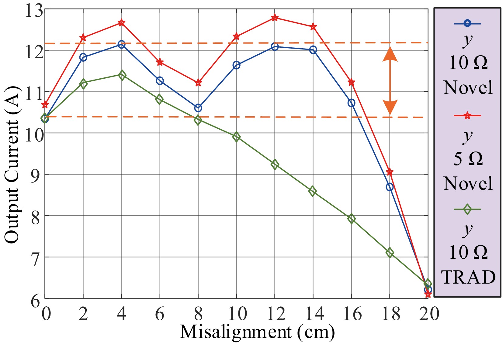
Figure 14. 

The curves of output current with coil misalignment.

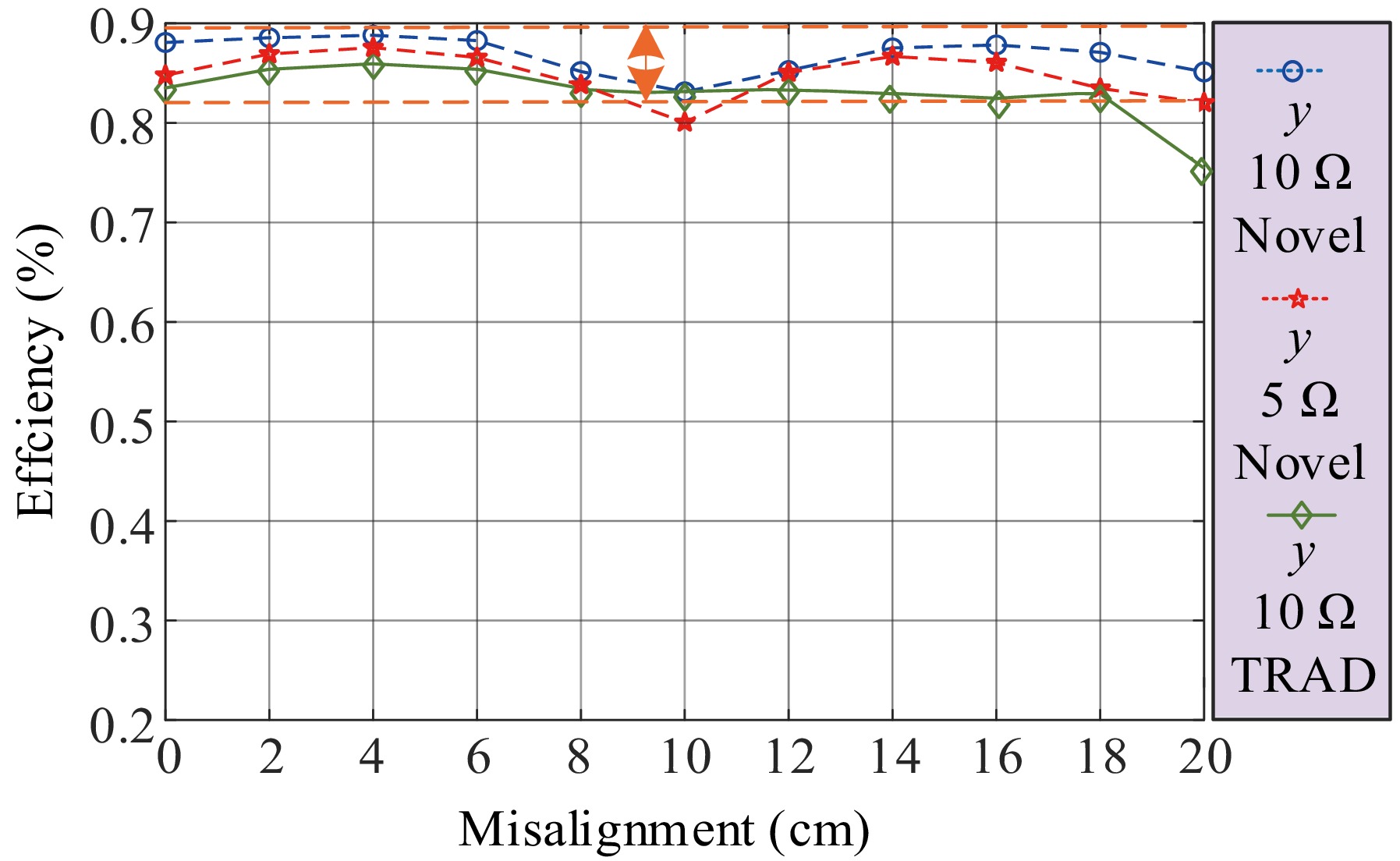
Figure 15. 

The curves of efficiency with coil misalignment.

In Fig. 14, when the misalignment is 16 cm, the current is equal to the current at the facing position. Within the misalignment range of 0–16 cm, the maximum output current is 12 A, the minimum value is 10.4 A, and the current fluctuation amplitude is 13.3%. The external dimensions of the magnetic coupling mechanism are 26.6 cm, with a misalignment of 16 cm accounting for 60% of the external dimensions. This is a large displacement distance, indicating that the method has strong displacement tolerance capability.

In Fig. 15, the maximum efficiency of the improvement methods is 89%. Within the 20 cm misalignment range, the system efficiency is always higher than 80%.

In Fig. 15, the green curve represents the primary side as the DD coil, and the secondary side is the traditional DDQ coil. The efficiency changes when displaced along the Y-direction. The improved efficiency curve is also higher than the traditional efficiency curve.

Although traditional DDQ coils solve the problem of rapid coupling zero-crossing when the DD coil is misaligned along the Y direction, they cannot reduce the coupling fluctuations during large-scale misalignment. The decoupling DDQ model proposed in this paper has small current fluctuations during large-scale misalignment and always maintains high efficiency.

Figure 16 shows the voltage and current waveforms of the inverter and the coil current in the facing position. It can be seen that the voltage and current of the inverter in the facing position are in the same phase, and there is no reactive power transmission.

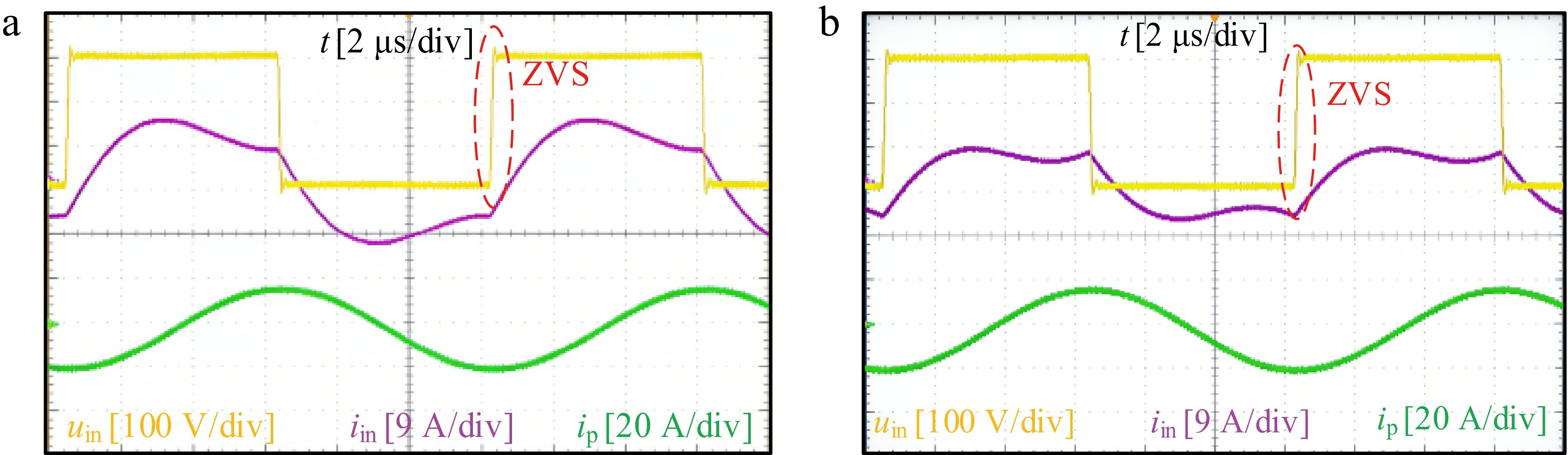
Figure 16. 

Experimental waveforms of inverter voltage, current, and coil current at the facing position. (a) 10 Ω. (b) 5 Ω.

Figure 17 shows the experimental waveform of three rectified voltages, currents, and coil currents on the secondary side in the facing position. In Fig. 17a and b, due to the decoupling of the Q coil on the secondary side and the DD coil on the primary side in the facing position, the rectified current is very small. The rectifier voltage and current of the pair of D coils on the secondary side are in phase. In the facing position, the Q coil of the secondary side is decoupled from the DD coil of the primary side. According to Eq. (2), the rectified input current is related to the mutual inductance, so the rectified current of the Q coil is in a discontinuous state at this time.

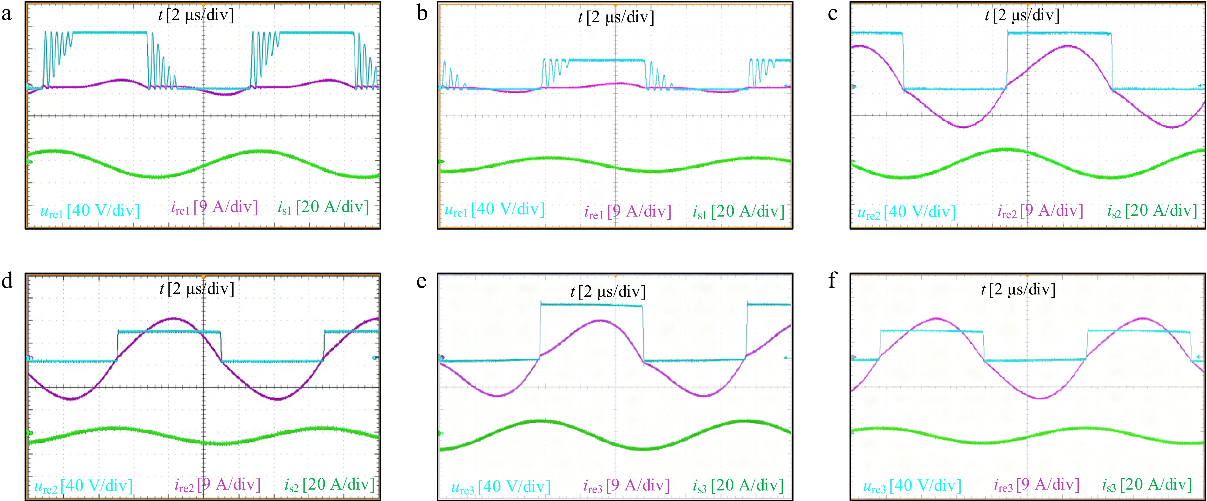
Figure 17. 

Experimental waveforms of rectifier voltage, current, and coil current in the facing position. (a) Secondary-side Q coil, 10 Ω. (b) Secondary-side Q coil, 5 Ω. (c) Secondary-side D coil, 10 Ω. (d) Secondary-side D coil, 5 Ω. (e) Another secondary-side D coil, 10 Ω. (f) Another secondary-side D coil, 5 Ω.

Figure 18 has similar content to Fig. 17, but with a misalignment of 8 cm along the Y direction. Figure 18c and d show one of the D coils on the secondary side. When misaligned by 8 cm, this D coil is decoupled from the DD coil on the primary side, thus exhibiting a discontinuous state similar to Fig. 17a and b. It is worth mentioning that, due to the symmetrical design of parameters, according to Eqs (1) and (2), the current of the secondary coil is equal; because three sets of half-bridge rectifiers are connected in parallel, the output voltage Uo is the same, and the parameter X1 is also the same. The rectified current is related to the mutual inductance.

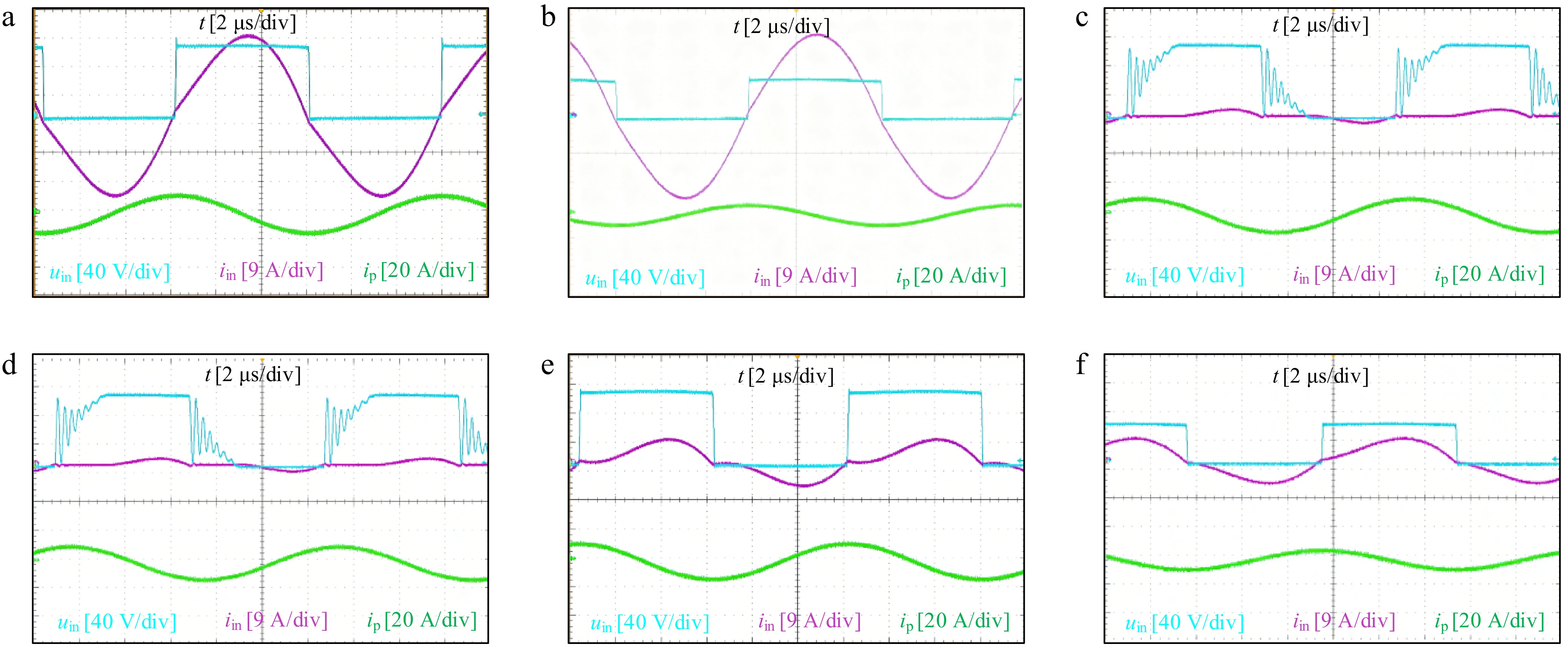
Figure 18. 

Experimental waveforms of rectifier voltage, current, and coil current with a misalignment position of 8 cm in the Y direction. (a) Secondary-side Q coil, 10 Ω. (b) Secondary-side Q coil, 5 Ω. (c) Secondary-side D coil, 10 Ω. (d) Secondary-side D coil, 5 Ω. (e) Another secondary-side D coil, 10 Ω. (f) Another secondary-side D coil, 5 Ω.

Figure 18 shows the system's adaptive switching state, which can achieve automatic switching according to different coupling states. Compared to the receiving end of a traditional DDQ coil, the DD coils of traditional DDQ coils are connected in reverse series and cannot automatically switch based on coupling. This demonstrates that the system has strong interoperability.

Figure 19 shows the inverter voltage and current with a misalignment of 8 cm along the Y direction, and the coil current diagram. It can be seen that the inverter voltage and current are in phase, and the system has no reactive power transmission under two load and misaligned conditions.

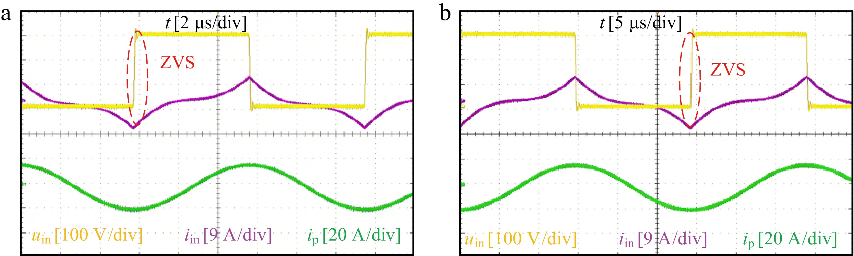
Figure 19. 

Experimental waveforms of inverter voltage, current, and coil current with a misalignment position of 8 cm in the Y direction. (a) 10 Ω. (b) 5 Ω.

The proposed receiver-side structure uses three LCC compensation branches to improve the misalignment tolerance of the DDQ receiver. Although this configuration improves the output-current stability under lateral misalignment, it also introduces additional loss components compared with a conventional single-branch receiver. Therefore, the loss distribution is analyzed to clarify the efficiency trade-off of the proposed method. The total system loss can be expressed as: P_loss = P_in – P_o, where P_in is the input power, and Po is the output power. The system efficiency is: η = P_o/P_in = P_o/(P_o + P_loss). The total loss can be approximately divided into: P_loss = P_inv + P_coil,p + P_coil,s + P_LCC/S + P_dec + P_rec + P_core, where P_inv is the inverter loss, P_coil,p is the primary coil copper loss, P_coil,s is the total copper loss of the three secondary coils, P_LCC/S is the loss of the three receiver-side LCC compensation branches, P_dec is the loss of the decoupling components, P_rec is the rectifier loss, and P_core is the magnetic core loss.

The additional loss of the proposed system mainly comes from the three receiver-side LCC branches, the secondary coil branches, and the diode rectifier. These losses reduce the peak efficiency compared with a simpler single-channel receiver. However, the proposed structure significantly improves the misalignment tolerance and output-current stability. Experimental results show that the output current fluctuation is only 13.3% within a lateral misalignment range of 60% of the coil outer dimension, and the system efficiency remains higher than 80% over the tested range. Therefore, the proposed method provides a trade-off between efficiency and misalignment tolerance. Further efficiency improvement can be achieved by adopting synchronous rectification, reducing the AC resistance of the coils and compensation inductors, and optimizing the LCC compensation parameters. The specific loss analysis diagram is shown in Fig. 20.

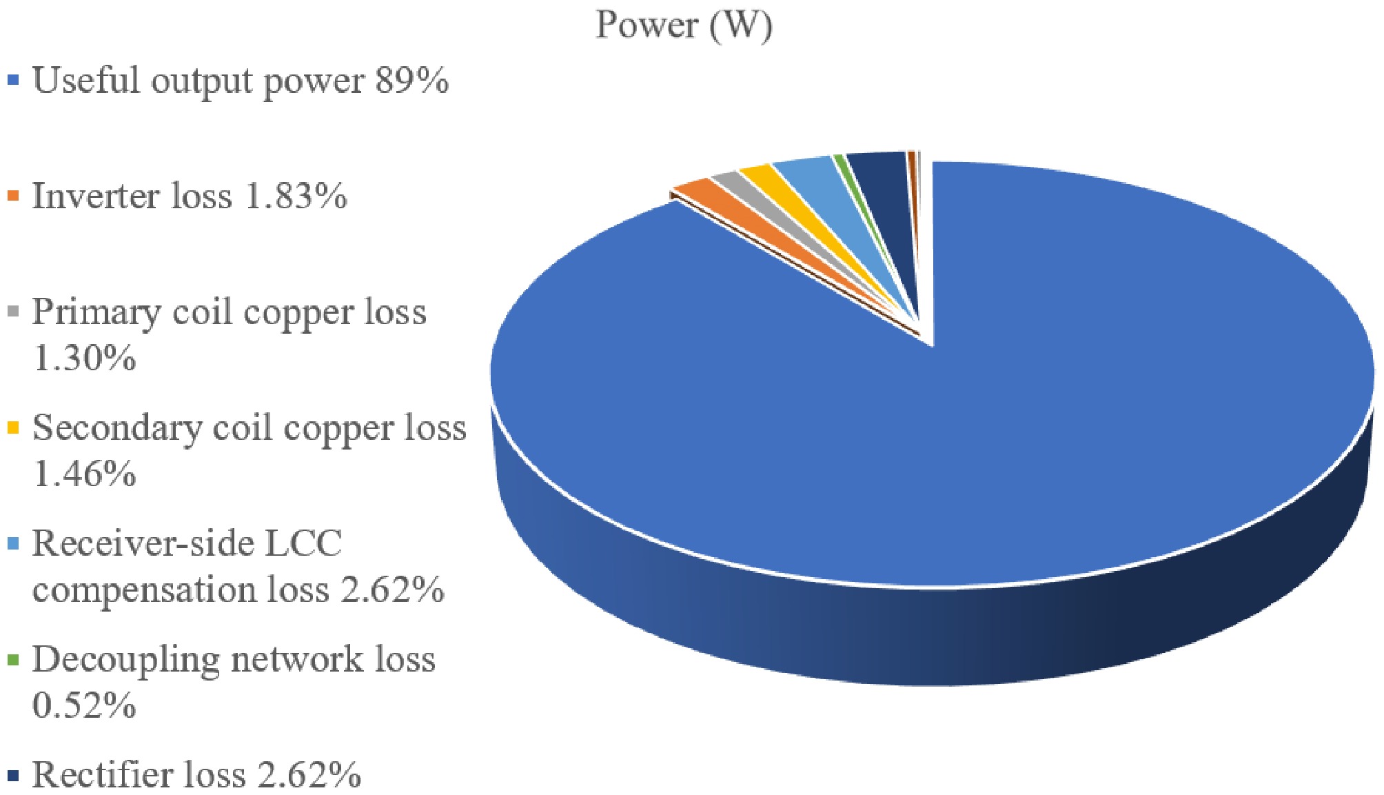
Figure 20. 

The specific loss analysis diagram.

To comprehensively evaluate the proposed decoupling model based on the DDQ coil, a systematic comparison with state-of-the-art solutions reveals distinct trade-offs among efficiency, complexity, and reliability (Table 2)^[20−22].

It should be noted that the systems listed in Table 2 were implemented with different power levels, magnetic coupler dimensions, air gaps, load conditions, and control strategies. Therefore, the absolute values of output power and efficiency cannot be used alone as a fully fair basis for comparison. To provide a more meaningful benchmark, the misalignment capability is also expressed in a normalized form, i.e., the maximum lateral misalignment divided by the outer dimension of the magnetic coupler. In addition, the output fluctuation and system complexity are included to reflect the practical trade-offs among misalignment tolerance, efficiency, hardware cost, and implementation difficulty.

From this normalized comparison, the proposed method does not aim to achieve the highest peak efficiency under a specific operating point. Instead, its main advantage lies in achieving a large normalized misalignment range with small output fluctuation using only passive decoupling components and a simplified rectifier structure. Compared with methods relying on hybrid topology switching, special coil structures, or reconfigurable rectifiers, the proposed system provides a lower-complexity solution for improving the misalignment tolerance and interoperability of DDQ-based WPT systems. Nevertheless, the present prototype still has limitations in peak efficiency, and further improvements can be expected by adopting synchronous rectification and optimizing the compensation parameters and coil structure.

Although the research method in this paper has some deficiencies in efficiency, the advantage is that the misalignment range is large while maintaining a high coupling coefficient, so that the output fluctuation is small. The method in this paper only changes the connection relationship between the coil and the compensation topology and adds passive components and a group of rectifier bridge arms to realize coil decoupling, so as to achieve strong anti-offset and interoperability. In addition, the goal of future work is to improve the efficiency by introducing a synchronous rectifier circuit, and further improve the system by optimizing the compensation topology parameters and coil structure to improve the offset tolerance.

The secondary-side DDQ coil is tapped at the center and connected in series with inductors and capacitors to achieve magnetic decoupling. Then, DDQ is connected to a novel rectifier topology that allows the absolute mutual inductance of the two D pads and Q coil relative to the primary coil to be added. Compared with the traditional DDQ coil, which solves the coupling zero-crossing problem of the DD coil by supplementing mutual inductance with the Q coil, the improved decoupled DDQ coil, based on the advantages of the traditional DDQ coil, enables a pair of D coils to adapt to magnetic field changes and change the current direction separately, thereby optimizing the output current curve when the Y direction is misaligned, making the output current fluctuation smaller and the efficiency higher. Therefore, the misalignment tolerance along the Y-axis is significantly improved, effectively simulating the behavior of automatic switching and enhancing interoperability. A 1.7 kW prototype was developed, and experimental results showed a maximum efficiency of 89%. Even within a 60% lateral displacement range relative to the length of the coil along the y-axis, the output current is higher than the rated value, with a variation amplitude of only 13.3%, and the efficiency is higher than 80%.