SRD: Sparse ramp discrimination for classification and variable selection on high-dimensional biological data

The rapid advancement of high throughput technologies has enabled the collection of diverse omics data generated through whole genome tiling arrays, mass spectrometry, and more recently next-generation sequencing platforms. While these massive data provide us with vast information, they also pose significant challenges for data analysis. One major issue is the high dimensionality of the data—for instance, microarray gene expression data can measure tens of thousands of genes simultaneously—coupled with the typically small sample sizes. This 'curse of dimensionality' makes it difficult to accurately estimate model parameters. Additionally, the inherent noise in biological data and the uncertainty in the target response often lead to overfitting, further complicating analysis.

Classification plays a pivotal role in biomedical and bioinformatics research^[1,2]. It involves learning a function from training data to predict the class label of any valid input covariates. The support vector machine (SVM) is one of the commonly used classification methods^[3−5]. However, SVMs cannot perform variable selection simultaneously, which is essential for analyzing high-dimensional data. Zhu et al.^[6] proposed the ℓ₁-norm SVM, which incorporates the LASSO penalty^[7] for automatic variable selection. Wang et al.^[8] applied the elastic-net penalty^[9] to SVMs for variable selection on high dimensional data. The elastic-net penalty exhibits a 'grouping effect', which tends to select or remove highly correlated covariates together.

Many large margin classification algorithms, including SVMs, are in the regularization framework, typically following the 'loss + penalty' format. In addition to the LASSO and elastic-net penalties, other penalties, such as ℓ_1/2^[10] and SCAD^[11], have also been applied to pattern classification in high-throughput biological data analysis.

In this work, we focus on the loss function. For binary classification problems, the most straightforward loss function is the 0-1 loss. However, it is well known that minimizing the 0-1 loss is NP-hard. As a result, surrogate loss functions are commonly used instead. Generally, loss functions can be categorized into two types: convex and non-convex.

Convex loss functions, such as the hinge loss used in SVMs, are computationally advantageous due to the convexity. However, the unbounded property of the convex function often leads to poor approximations to the 0-1 loss function. To address this limitation, various non-convex loss functions have been proposed, including the Ψ loss^[12], the ramp loss^[13,14], and the sigmoid loss^[15,16]. Non-convex loss functions, such as the ramp loss, are particularly robust to outliers^[14]. In contrast, convex loss functions can be sensitive to outliers, making the corresponding classifiers prone to being dominated by outliers.

The robustness of non-convex loss functions makes them well-suited for handling noisy, high dimensional biological data. However, non-convex optimization poses significant challenges. In this work, we use a smoothed version of the ramp loss function, and propose applying the difference of convex (d.c.) algorithm to efficiently solve the non-convex optimization problem through a sequence of convex subproblems. We refer to the proposed method as Sparse Ramp Discrimination (SRD).

Consider n training data pairs: {(x_i, y_i), i = 1, ... ,n}, where x_i is a d-dimensional covariate vector representing the i' th sample, and y_i $ \in \ ${1, −1} is the corresponding class label. The linear decision function is described as:

where, β = (β₁, ..., β_d)_T, and β₀ is a scalar. The decision function divides the covariate space into two regions based on the sign of f(x).

Many large margin classification methods, such as SVMs, fall in the regularization framework, where the objective function is constructed in the form of 'loss + penalty' as follows:

where, L(·) is a loss function and p_λ(·) is a penalty function with regularization parameters λ. For binary classification problems, the most straightforward loss function is the 0-1 loss $ L\left(r\right)=\mathbb{I}\left(r < 0\right) $, where $ \mathbb{I}\left(\cdot \right) $ is the indicator function. The well-known SVMs use the hinge loss, L(r) = max(1−r, 0), and the ridge penalty, $ {p}_{\lambda }\left(\beta \right)=\dfrac{\lambda }{2}{\beta }^{2} $. Although SVMs are widely applied in bioinformatics for high-dimensional data analysis, they do not support automatic variable selection. Traditional variable selection methods, such as recursive feature elimination
(SVM-RFE)^[5,17], are computationally intensive and often lack stability^[18].

Zhu et al.^[6] proposed the ℓ₁-norm SVM, which uses the LASSO penalty, $ {p}_{\lambda }\left(\beta \right)=\lambda \left|\beta \right| $^[7] for automatic variable selection. However, the LASSO penalty has two notable limitations: (1) the number of selected variables is constrained by the sample size; (2) the LASSO penalty tends to select only one or a few highly correlated variables. To address these issues, Wang et al.^[8] applied the elastic-net penalty^[9], defined as:

where, λ₁, λ₂ ≥ 0 are regularization parameters. The elastic-net penalty represents an important generalization of the LASSO penalty. As a hybrid of the LASSO and ridge penalties, the elastic-net penalty retains the variable selection feature of LASSO while introducing a grouping effect, a characteristic of the ridge penalty. This grouping effect ensures that highly correlated variables are likely to be selected or removed together, resulting in similar estimated coefficients for such variables.

Sparse ramp discrimination

The loss functions in Eqn (1) can be categorized into two types: convex and non-convex. An example of a convex loss function is the hinge loss used in SVMs. It serves as a convex upper bound of the 0-1 loss function. The convexity makes the optimization algorithm computationally efficient. However, the unbounded nature of convex loss functions often results in a poor approximation of the 0-1 loss.

On the other side, non-convex loss functions, such as the ramp loss^[14], provide better approximations to the 0-1 loss. It is well known that by truncating the unbounded hinge loss, ramp loss-related methods have been shown to be robust to outliers in training data for classification problems^[14]. The robustness makes non-convex loss functions suitable for handling noisy high dimensional biological data. However, the non-convex optimization is challenging, which often limits their practice application. Here we consider a novel non-convex loss function:

We refer to this as the smoothed ramp loss in this article. Figure 1 illustrates the hinge loss, ramp loss, and smoothed ramp loss functions. Unlike the ramp loss, the smoothed ramp loss is differentiable everywhere, providing computational advantages for optimization. Moreover, similar to the ramp loss, the smoothed ramp loss is also robust to outliers.

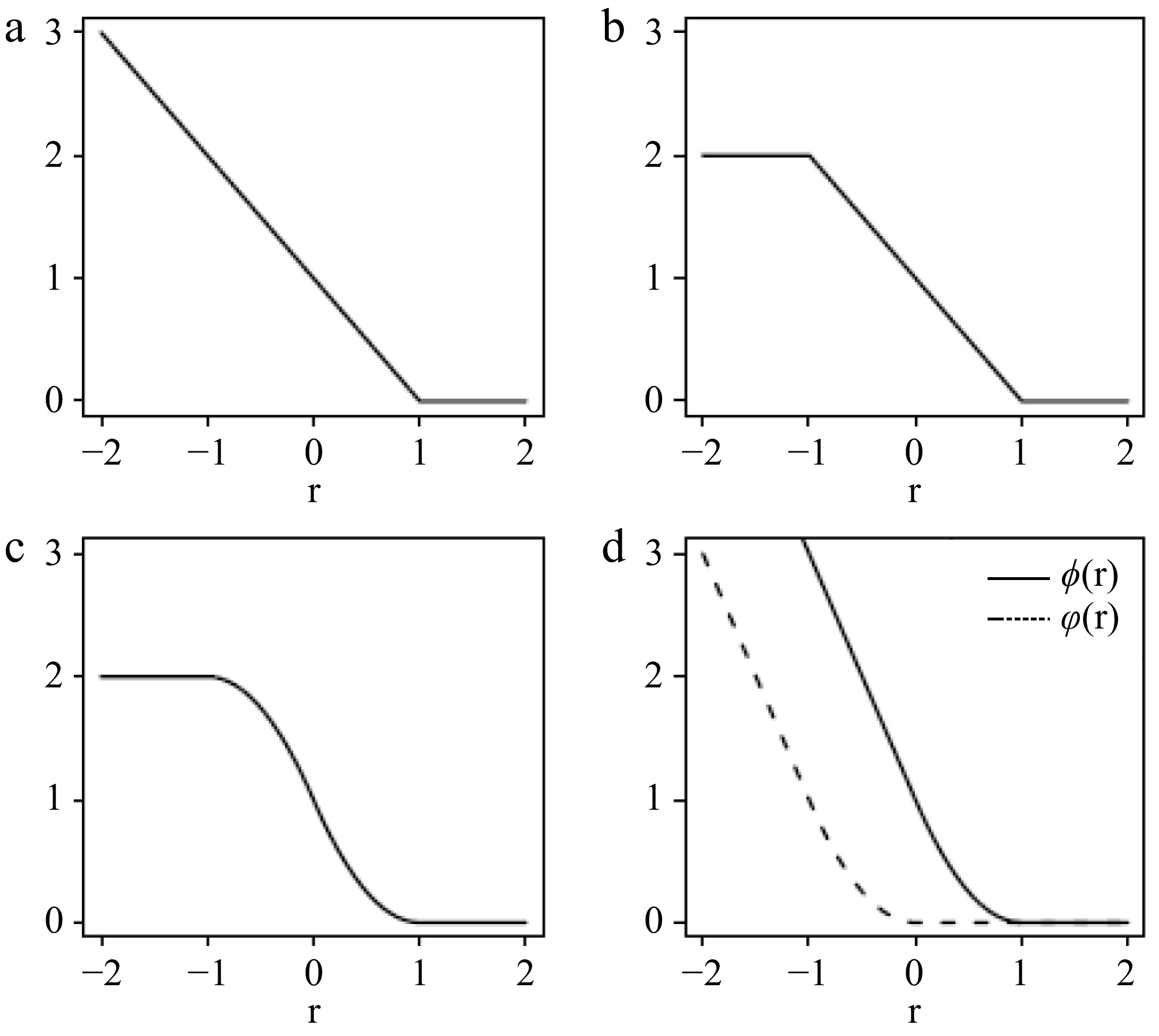
Figure 1. 

(a) Hinge loss, (b) ramp loss, and (c) smoothed ramp loss functions. (d) Shows the difference of convex decomposition of the smoothed ramp loss, T(r) = ϕ(r) − $\varphi $(r).

In this work, we integrate the smoothed ramp loss with the elastic-net penalty into the regularization framework in Eqn (1), and propose a novel method called sparse ramp discrimination (SRD):

Here we only present a case where all covariates are penalized using the same parameters λ₁ and λ₂. In practice, different values of λ₁'s or λ₂'s can be assigned to individual covariates.

Note that T(·) is Lipschitz continuous with a Lipschitz constant of 2. According to Theorem 1 in Wang et al.^[8], SRD has the grouping effect. For the sake of completeness, we restate the theorem for SRD in this article.

Theorem 1. Let $ \hat{\mathbf{{\boldsymbol{\beta}} }} $ and $ {\hat{\beta }}_{0} $ denote the solution for (3). For any pair (j, j'), we have

Furthermore, if the input covariates x._j = (x_1j, ..., x_nj)^T and x._j' = (x_1j', ..., x_nj')^T are centered and normalized, then

Theorem 1 demonstrates that highly correlated covariates tend to have similar estimated coefficients. As a result, they are more likely to be selected or removed together, particularly when λ₂ is large.

Algorithm

The smoothed ramp loss is a non-convex loss function, which makes the optimization problem in Eqn (3) a non-convex minimization task. Similar to the robust truncated hinge loss SVM^[14], we solve the non-convex minimization problem using the d.c. algorithm^[19], also known as the Concave-Convex Procedure (CCCP) in the machine learning community^[20]. This approach assumes that the objective function can be expressed as the sum of a convex component, Q_vex(Θ), and a concave component, Q_cav(Θ). As outlined in Algorithm 1, the d.c. algorithm solves the non-convex optimization problem by minimizing a sequence of convex subproblems.

Let

Note that both $\varphi $(·) and ϕ(·) are smooth and convex. We have a difference-of-convex decomposition of the smoothed ramp loss,

as illustrated in Fig. 1d. Denote Θ as (β, β₀). Applying Eqn (4), the objective function in Eqn (3) can be decomposed as:

where, the margin $ {r}_{i}={y}_{i}\left({\mathbf{x}}_{i}^{T}\mathbf{\beta }+{\beta }_{0}\right) $. To simplify, we introduce the notation,

for i = 1, ..., n. Thus, the convex subproblem at the (t + 1)'th iteration of the d.c. algorithm is:

It is popular to use coordinate descent methods to solve such optimization problems^[21,22]. However, under some circumstances, coordinate descent methods may suffer from slow convergence. In this work, we apply the General Iterative Shrinkage and Thresholding (GIST) algorithm^[23]. GIST updates all coordinates simultaneously through gradient descent and a thresholding rule, and it is easy to implement. We do not delve into the details of GIST in this article. Interested readers may refer to Gong et al.^[23]. The SRD procedure is summarized in the following algorithm:

The algorithm is not limited to the smoothed ramp loss. It is applicable to a broader class of smooth non-convex loss functions that can be similarly expressed using a difference-of-convex decomposition, as shown in Eqn (4). For instance, the logistic sigmoid loss function^[16], s(r) = 1/{1+ exp(r)}, can also be used in this framework. It is easy to verify its difference-of-convex decomposition as s(r) = ϕ'(r) − $\varphi $'(r), where:

Implementation

We have implemented Algorithm 2 in the R package SRDnet. SRD involves two tuning parameters λ₁ and λ₂. λ₁ plays a more significant role in variable selection, making the performance highly sensitive to its value.

We first generate a pre-specified set of λ₂ values by ignoring λ₁ and using a similar procedure as in SVMs. Then for each pre-specified λ₂, we compute the solution path using a fine grid of λ₁ values to achieve better tuning for λ₁. We start with finding λ_max, which is the smallest λ₁ that sets β = 0. According to the Karush-Kuhn-Tucker (KKT) conditions^[24], λ_max satisfies at least one of the following inequalities,

for j =1, ..., d. Let $\tilde{\lambda } $_max = max_j$\tilde{\lambda } $_max,j. We first set λ₁ = $\tilde{\lambda } $_max and gradually decrease λ₁ in Algorithm 2 to locate λ_max. We set λ_min = τλ_max, where τ is a user-defined quantity. The default value of τ is τ = 0.01 for n < d data and τ = 0.0001 for n ≥ d data. Between λ_min and λ_max, we place K points uniformly in the log-scale. The default value for K is 98 such that the solution path has 100 λ₁ values. A warm-start trick, as in GCDnet^[22], is also implemented. Specifically, for computing the solution of the (k + 1)'th λ₁, the solution at the k'th λ₁ is used as the initial value in Algorithm 2.

In this section, we conducted simulation studies to evaluate the performance of the proposed SRD method. The training data consisted of 100 subjects (50 cases and 50 controls), where each input x was a d = 500-dimensional vector. Independent tuning and testing data were generated in the same way as the training data. The sample sizes for the tuning and testing data were 100 and 10,000, respectively. The tuning data were used to select the optimal tuning parameters via a grid search, and the testing data were used to evaluate the accuracy of various classification methods.

We considered two scenarios similar to those in Wang et al.^[25]. In the first scenario, all covariates are independent. The '+' class follows a normal distribution with a mean of:

and a covariance matrix $ \mathbf{\Sigma }={\mathbf{I}}_{d\times d} $. The '−' class follows a similar distribution except that the mean is:

The Bayes optimal classification rule depends solely on the first 10 covariates, with a Bayes error of 5.69%. The second scenario represents an example where the relevant covariates are correlated. The '+' class follows a normal distribution with a mean of:

and a covariance matrix:

where, the diagonal elements of $ {\mathbf{\Sigma }}^{\mathrm{*}} $ are 1 and all off-diagonal elements are 0.8. The '−' class has a similar distribution except that the mean is:

The Bayes optimal classification rule depends only on the first 10 highly correlated covariates, and its Bayes error is 13.47%.

We compared the standard SVM, hybrid huberized SVM (HHSVM)^[25], and the proposed SRD method. HHSVM uses a smoothed hinge loss, called huberized hinge loss, combined with an elastic-net penalty. SVM was implemented using the e1071 R package, and the R package GCDnet^[22] was used for HHSVM.

We used the tuning dataset to select the tuning parameters for each method. For SVM, we searched over a pre-specified set of tuning parameter values for C, and selected the one that minimized the prediction error on the tuning data. For HHSVM and SRD, we chose a pre-specified set of λ₂ values, and adaptively determined a fine grid of λ₁ values using the procedure described in the methods, with τ = 0.01 and K = 98. The best pair (λ₁, λ₂) was selected based on the smallest prediction error on the tuning data. The performance of the selected models was then evaluated on independent testing data. Each experiment was repeated 1,000 times.

The mean prediction errors and corresponding standard deviations (in parentheses) are summarized in Table 1 (first two rows). As shown in Table 1, the prediction errors of SRD and HHSVM are similar, and outperform those of SVM in both scenarios. This improvement is attributed to the variable selection mechanism employed by SRD and HHSVM. Unlike SVM, which uses all covariates and is thereby affected by noise covariates, SRD and HHSVM are more robust due to their ability to select relevant features. The similar performance of SRD and HHSVM in scenario 2 highlights that SRD effectively identifies all correlated relevant covariates, a result of the 'grouping effect' provided by the elastic-net penalty, as in HHSVM.

The computation of SRD is higher than that of HHSVM due to the nature of non-convex optimization. At our computational facility, HHSVM took approximately 26.6 min for scenario I with 1,000 repeats. In contrast, with the same number of pre-specified (λ₁, λ₂) pairs for tuning, SRD took approximately 145.2 min for 1,000 repeats.

We perturbed the training data by randomly selecting perc(10% or 20%) of the samples and flipping their class labels to the opposite. We repeated the above testing procedure on the perturbed training data. The results are also presented in Table 1. The performance of all methods deteriorated due to the perturbation. However, SRD was the least affected, as expected. This supports our claim that the non-convex smoothed ramp loss enhances the robustness of the model compared to convex loss functions, leading to more accurate classifiers in the presence of outliers in the training data.

We also compared the covariates selected by HHSVM and SRD (SVM retains all covariates). We consider q_signal, the number of selected relevant covariates, and q_noise, the number of selected noise covariates. The results are presented in Table 2. When there is no perturbation in the training data, both HHSVM and SRD perform similarly. However, in the presence of perturbation, SRD tends to select more relevant covariates. Despite this, both methods also select a significant number of noise covariates. One way to further remove the noise covariates is to use tuning methods that favor more parsimonious models. For example, applying the 'one-standard error' rule^[26] during cross-validation for parameter tuning has proven effective in screening out noise.

In this section, we investigated the performance of SVM, HHSVM, and our proposed SRD method using microarray gene expression data from a colon cancer study^[2]. This dataset includes 62 samples, consisting of 40 colon cancer tumors and 22 normal tissues. Each sample contains expression measurements for 2,000 genes obtained using an Affymetrix gene chip. The data are publicly available.

We pre-processed the data following the procedure described by Dudoit et al.^[27]. Microarray gene expression levels below the minimum threshold of 100 were set to 100, and the maximum threshold was capped at 16,000. We excluded genes with max/min ≤ 5 and (max − min) ≤ 500, where max and min denote the maximum and minimum expression levels of a gene across samples. The expression levels were then logarithmically transformed. After thresholding, filtering, and logarithmic transformation, the data were standardized to have a zero mean and unit standard deviation for each gene. The pre-processed data (p = 1,224) were used for all subsequent analysis. It has been reported that five samples (three tumors and two normal tissues) were contaminated^[28], making this dataset particularly suitable for assessing the robustness of the proposed SRD method.

We compared the performance of SVM, HHSVM, and SRD. All methods involve at least one tuning parameter. We used 10-fold cross-validation to select the optimal parameters. Since the sample size is small, the cross-validation error is known to have high variance. To mitigate this, we repeated the cross-validation procedure ten times and averaged the cross-validation errors to reduce the variance. We selected the parameter with the smallest average cross-validation error. This tuning strategy is referred to as the optimal rule in this article. For HHSVM and SRD, we aimed to choose a parsimonious model if its prediction performance was not compromised too much. A common approach, the 'one-standard error' rule^[26] is used in cross-validation to select the most parsimonious model whose prediction error is no more than one standard error above the optimal error. In this work, we used a slightly different way to compute the standard error to incorporate into the repeated cross-validation procedure. That is, the standard error was computed through the individual prediction error rates for each of the ten repetitions. Here, we applied both tuning strategies: the optimal rule and the 'one-standard error' rule.

To evaluate classification performance, we conducted a nested 10-fold cross-validation procedure^[29]. The data were randomly partitioned into ten roughly equal-sized folds. In each iteration, nine folds were used as training data, where an internal cross-validation procedure was performed to tune the model parameters. The classification model was then trained on the full training set using the selected parameters and applied to predict class labels for the left-out fold. This process was repeated nine more times to obtain predictions for all folds, yielding the overall prediction error. For a reliable evaluation of prediction accuracy, we repeated the outer cross-validation procedure 100 times with different fold partitions. The average and standard deviation of these 100 prediction errors are reported in Table 3. During the cross-validation procedure with 100 repetitions, we trained a total of 1,000 classification models for each method. For HHSVM and SRD, the average number of selected genes is also reported in Table 3.

We can see that SRD seems to have a better classification accuracy than HHSVM. It confirms again the robustness of SRD in classification and variable selection when there exist outliers in the training data. Interestingly, SVM performed similarly with SRD although SVM used all covariates. The reason perhaps is that the gene expression levels are highly correlated for many genes. The correlation enhances the signal. In the simulation studies, both scenarios have ten relevant covariates, and the only difference is that in scenario II the relevant covariates are highly correlated. SVM performed much better in scenario II than in scenario I.

We used two tuning strategies. From Table 3, the 'one-standard error' rule is effective to select a parsimonious model without sacrificing too much on the prediction accuracy. We investigated the genes selected in the 1,000 SRD models determined by the 'one-standard error' rule during the cross-validation procedure. The top 20 most frequently selected genes are listed in Table 4.

The molecular carcinogenesis of colorectal cancer is complex and poorly understood. Some comments about the top frequently selected genes are worthy of mention. MYH9 and its regulatory MYL9 are components of the cytoskeletal network involved in actomyosin-based contractility and implicated in the invasive behavior of tumor cells^[30]. hnRNP A1, a major member of the hnRNP family, binds to G-rich repetitive sequences and quadruplex structures in DNA. The overexpression of hnRNP A1 in colorectal cancer cells leads to evasion of cancer cell apoptosis^[31]. Uroguanylin, encoded by GUCA2B, is markedly down-regulated in adenocarcinomas of the colon, and the treatment with uroguanylin leads to induction of apoptosis in human colon carcinoma cells in vitro^[32]. S100P overexpressed in colorectal carcinomatous tissues, and the overexpression is significantly correlated with tumor metastasis, advanced clinical stage, and recurrence^[33].

In this article, we have proposed the Sparse Ramp Discrimination (SRD) method, which leverages the smoothed ramp loss to assess the 'badness-of-fit' and incorporates the elastic-net penalty for automatic variable selection. We apply the difference of the convex (d.c.) algorithm to efficiently solve the non-convex optimization problem through a sequence of convex subproblems. From the simulation studies and real data analysis, SRD is robust to outliers, making it particularly well-suited for handling noisy, high dimensional biological data.