Research on 4D trajectory prediction methods for aircraft in point merge approach mode

The International Air Transport Association predicts that the world's route volume will continue to grow. The contradiction between the rapidly growing demand for air transportation and limited airspace is prominent, leading to increasingly severe congestion in airport terminal areas^[1]. Trajectory Based Operation (TBO), as a set of system-level solutions proposed by the civil aviation community in recent years, aims to improve the ATC system protection capability and operational efficiency, and its improvement in high-density airspace operation is mainly oriented to improve the automation capability, which is divided into three main parts: Four Dimensional (4D) trajectory prediction system, conflict detection and resolution system, and route surveillance system^[2]. Among them, the 4D trajectory prediction system is the cornerstone of TBO air route management, and its importance is self-evident^[3].

In the research of trajectory prediction, the method based on multiple linear regression has been used for a long time. For example, Kalman filtering^[4], linear^[5], or Gaussian regression models^[6,7], time series analysis^[8], and autoregressive models^[9] to optimize hand-crafted energy functions are gradually emerging and developing. In 2018, Shiz et al.^[10] implemented trajectory prediction based on long and short-term memory networks. Wang & Huang^[11] realized trajectory prediction based on the Kalman filtering algorithm and improved the algorithm, which improves the accuracy of trajectory prediction by identifying system noise. Han et al.^[12] designed a parameter evolution model for aircraft to plan conflict-free 4D trajectories by adjusting the flight parameters of the aircraft. Linear models are difficult to apply in complex nonlinear motion trajectories, and neural networks have achieved better results in trajectory prediction due to their better ability to learn nonlinearities.

In point merge research, in 2006, the Norwegian Air Traffic Control proposed the concept of point merge, which improves the prediction accuracy of aircraft arrival moments and airspace capacity. Ivanescu et al.^[13] in 2009 confirmed that the point merge approach model improves aircraft descent profiles, and reduces the amount of controller and pilots' call volume, which is suitable for high traffic operational environment. Chao et al.^[14] and designed a point merge approach procedure for Changsha Huanghua Airport in 2016 and summarized the design method of the point merge mode, and the dynamic and static capacity calculation methods within the point merge system. Li^[15] also studied the feasibility of the point merge procedure at Chongqing Jiangbei International Airport. Ma et al.^[16] took the point merge procedure at Shanghai Pudong International Airport as an example to discuss the impact of design parameters on the operation and environmental benefits of point merge systems, conducting computer simulations with a 4D trajectory prediction model to evaluate the operational effectiveness of point merge systems.

In this paper, a 4D trajectory prediction method for aircraft in point merge approach mode is proposed in response to the pressure brought by the increasing air traffic demand. Firstly, while retaining the flight characteristics of the aircraft, data preprocessing is carried out based on the principle of point merge. Secondly, the point merge data is screened out by dividing the route data. Finally, the simulation results of the two models, CNN (Convolutional Neural Network) and LSTM (Long Short-Term Memory), are compared and analyzed in terms of time, longitude, latitude, and altitude.

The point merge system is an air traffic management technology procedure applied in civil aviation to improve route safety. The technology achieves optimized route approach sequencing by sequencing aircraft according to temporal and spatial requirements and directing them to the merge point.

The point merge procedure mainly consists three important components: merge points, sequencing legs, and positioning points. Merge points are used to merge traffic flows and form a relatively unified traffic flow. Sequencing legs ensure that the distance from any point to the merge point is equal. The positioning points are to ensure that the aircraft establishes a safe interval within the point merge procedure. The schematic diagram of the point merge approach illustration is shown in Fig. 1.

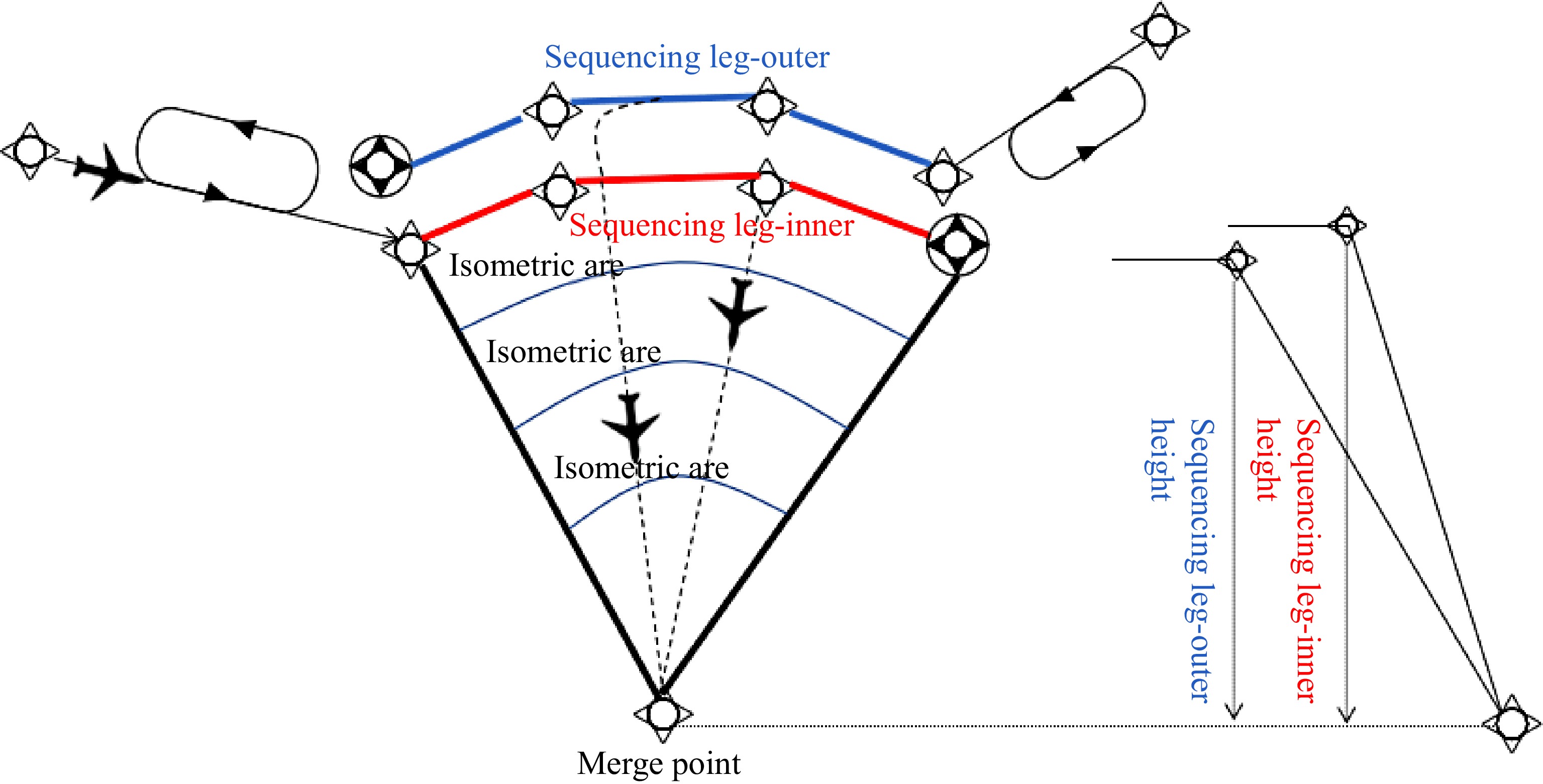
Figure 1. 

Point merge approach procedure.

The basic working principle of the point merge system is to guide routes originally dispersed in different radial directions to a point in an orderly manner. The controller only needs to issue the command of leaving the sorting edge and flying directly to the merge point to the aircraft at the right time, and there is no need to adjust the aircraft's heading, speed, and altitude frequently.

Continuous Descent Operations (CDO) can be combined with point merge mode to further improve the efficiency and safety of route approach. By using CDO, the landing altitude and descent rate can be well controlled under the guidance of the point merge system, which reduces delays and flight conflicts.

Data preprocessing

In this paper, the ADS-B data of 28,649 routes for 7 months from 2021 to 2022 in a certain airport are firstly partitioned into different CSV files corresponding to different routes based on the route number, which is convenient for the subsequent route mapping, screening, and prediction.

Redundant features are deleted from the segmented files, and the files are sorted according to the time sequence, which is convenient for subsequent route mapping, screening, and forecasting, and the time stamps are converted to Coordinated Universal Time (UTC) for easy reading and inspection. The different date routes of the same route name were segmented to obtain the navigation parameters such as longitude, latitude, altitude, speed, and vertical speed of each route for each day.

This passage focuses on trajectory prediction in point merge approach mode, and the data of departure routes, and cruise phase should be excluded during data screening. The distance between the latitude and longitude of the last line of each route and the Aerodrome Reference Point (ARP) coordinates of a certain airport is calculated to determine whether the end point is near the airport. For the data culling in the cruise phase and the labeling screening of point merge approach routes, the route data are selected to be screened by observing them in the range of the terminal area.

The final screening from 28,649 routes, eliminating nearly half of the departure routes, and then processing the resulting approach routes, removing other ways to approach the routes, selecting the point merge approach routes, and ultimately obtaining 596 point merge routes, in order to facilitate the intuitive display of the overall route characteristics of the routes on different dates of the unified processing of the times, drawing the time−altitude illustration.

Data set partitioning and training preparation

The 596 point merge routes screened are divided into: 70% training set, 20% validation set, and 10% test set. In addition to this, in order to maintain the continuity of the data, the time series are harmonized and sorted before dividing the dataset. After dividing the dataset, ensure that a sliding window is applied to each subset (training, validation, and testing). The data also needs to be preprocessed and normalized before input to the model. After creating the sliding window data for all the routes, merge them into one large input matrix and output matrix for input into the deep learning model. Iterate through all the routes and create sliding window data for each route and then stack them together and feed them into the deep learning model for training and prediction after preparing the input and output data.

Model training and results analysis

CNN model

CNN is a deep learning model commonly used in the field of image processing and computer vision. CNN is a hierarchically structured neural network whose main purpose is to perform tasks such as classification, recognition, and segmentation of multidimensional data such as illustration. CNN mainly consists of convolutional, pooling, and fully-connected layers.

The convolutional layer is one of the most important components of CNN. It uses a convolution kernel (also called a filter) to perform a convolution operation on the input image to extract features. The pooling layer is used to reduce the size of the feature map while preserving the features. It is achieved by performing aggregation operations on small regions in the feature map. The main role of the pooling layer is to reduce the dimensionality of the feature illustration and reduce the amount of computation, while improving the robustness of the features. The fully connected layer is used to classify or regress the features extracted from the previous convolutional and pooling layers.

LSTM model

LSTM is a common RNN (Recurrent Neural Network) model which is commonly used to process sequential data, such as time series, text, etc. The main feature of LSTM is that it adds memory units, input gates, forgetting gates, and output gates on top of RNNs to achieve better memory and selective forgetting of information.

The core idea of the LSTM model is to control the flow of information through a gating mechanism, where each time step receives inputs from the current time step, as well as the hidden and memorized states from the previous time step. The gating mechanism controls the processes of input, forgetting, and output through a series of neural networks, thus realizing the selective processing of information.

Model training

The route data are read from different CSV files. The data contains information such as time, longitude, latitude, altitude, heading angle, ground speed, and vertical speed of the route. The dataset is divided using stratified sampling, where 70% of the data is used as a training set, 20% as a validation set, and 10% as a test set.

In the data preprocessing phase, for each route, the input features (including time, longitude, latitude, altitude, velocity, vertical velocity, and angle) and output features (including time, longitude, latitude, and altitude) are first determined. Second, the data is divided into training samples and corresponding labels based on the given time step. In this paper, a time series of length 16 is extracted as input features using the sliding window method, and the longitude, latitude, and altitude of the 17^th time step are used as the target outputs so that the trajectory prediction problem is transformed into a univariate single-step short-time prediction problem. Next, the input features are normalized for model training. In building the model, the Keras framework is used to construct a sequential model.

The specific parameters of CNN are listed as follows: two convolutional layers, each with 32 convolutional kernels, with kernel sizes of 2 and 1. The pooling window size of the one-dimensional max pooling layer is 2, and the number of neurons in the fully connected layer is 50. The specific parameters of LSTM are listed as follows: the number of hidden layer units is 50, the loss function of the model is chosen as mean square error, and the optimizer uses an Adam optimizer with a learning rate of 0.001.

When training the model, an early stopping strategy is used, by monitoring the loss values on the validation set. If the loss values do not improve significantly during 10 consecutive rounds of training, the training is stopped early and the optimal weights are restored. The training process for the different models only requires changes to the introduced libraries and the model-building section.

After the training is completed, the models are evaluated by using a test set. The outputs predicted by the models are back-normalized with the true outputs. Evaluation metrics such as Root Mean Square Error (RMSE), Mean Absolute Error (MAE), Mean Absolute Percentage Error (MAPE), Evaluation indicators include Average Horizontal Displacement Error (AHDE), Final Horizontal Displacement Error (FHDE), Average Vertical Displacement Error (AVDE), and Final Vertical Displacement Error (FVDE) are calculated between the predicted results and the actual data.

Next, the loss during training and the validation loss are visualized to observe the convergence of the model. The predicted values are plotted against the actual values to visualize the performance of the model in predicting longitude, latitude, and altitude. Finally, the predictions are saved to a CSV file and the trained model is saved as an HDF5 format file for subsequent use.

RMSE measures the deviation between the predicted and actual values, and the smaller its value is, the better the prediction performance it shows. The formula is shown in Eqn (1).

where, A_i is the actual value, P_i is the predicted value, and n is the number of observations. Equations (2) and (3) are identical.

MAE measures the deviation between predicted and actual values, and the smaller its value, the better the prediction performance. The difference with RMSE is that MAE is not sensitive to outliers, while RMSE is sensitive to outliers. The formula is shown in Eqn (2).

MAPE measures the size of the prediction error relative to the actual value and is often used to measure the relative degree of prediction bias, the smaller its value is, the better the prediction performance it shows. The formula is shown in Eqn (3).

AHDE refers to the average horizontal Euclidean distance between each predicted trajectory point and the actual trajectory point. The smaller the value, the better the prediction performance. The formula is shown in Eqn (4).

FHDE refers to the horizontal Euclidean distance between the last predicted trajectory point and the actual trajectory point. The smaller its value, the better the prediction performance. The formula is shown in Eqn (5).

AVDE refers to the average vertical Euclidean distance between each predicted trajectory point and the actual trajectory point. The smaller the value, the better the prediction performance. The formula is shown in Eqn (6).

FVDE refers to the vertical Euclidean distance between the last predicted trajectory point and the actual trajectory point. The smaller its value, the better the prediction performance. The formula is shown in Eqn (7).

In Eqns (4) to (7) above, $ {\mathrm{P}}_{\mathrm{i}}^{\mathrm{l}\mathrm{o}\mathrm{n}} $, $ {\mathrm{P}}_{\mathrm{i}}^{\mathrm{l}\mathrm{a}\mathrm{t}} $ and $ {\mathrm{P}}_{\mathrm{i}}^{\mathrm{a}\mathrm{l}\mathrm{t}} $ respectively represent the longitude, latitude, and altitude of the predicted trajectory point. $ {\mathrm{A}}_{\mathrm{i}}^{\mathrm{l}\mathrm{o}\mathrm{n}} $, $ {\mathrm{A}}_{\mathrm{i}}^{\mathrm{l}\mathrm{a}\mathrm{t}} $ and $ {\mathrm{A}}_{\mathrm{i}}^{\mathrm{a}\mathrm{l}\mathrm{t}} $ respectively represent the longitude, latitude, and altitude of the actual trajectory point; $ {\mathrm{P}}_{\mathrm{f}\mathrm{i}\mathrm{n}\mathrm{a}\mathrm{l}}^{\mathrm{l}\mathrm{o}\mathrm{n}} $, $ {\mathrm{P}}_{\mathrm{f}\mathrm{i}\mathrm{n}\mathrm{a}\mathrm{l}}^{\mathrm{l}\mathrm{a}\mathrm{t}} $ and $ {\mathrm{P}}_{\mathrm{f}\mathrm{i}\mathrm{n}\mathrm{a}\mathrm{l}}^{\mathrm{a}\mathrm{l}\mathrm{t}} $ represent the longitude, latitude, and altitude of the last predicted trajectory point. $ {\mathrm{A}}_{\mathrm{f}\mathrm{i}\mathrm{n}\mathrm{a}\mathrm{l}}^{\mathrm{l}\mathrm{o}\mathrm{n}} $, $ {\mathrm{A}}_{\mathrm{f}\mathrm{i}\mathrm{n}\mathrm{a}\mathrm{l}}^{\mathrm{l}\mathrm{a}\mathrm{t}} $ and $ {\mathrm{A}}_{\mathrm{f}\mathrm{i}\mathrm{n}\mathrm{a}\mathrm{l}}^{\mathrm{a}\mathrm{l}\mathrm{t}} $ respectively represent the longitude, latitude, and altitude of the last actual trajectory point.

In addition, the prediction results can be subsequently visualized by plotting the comparison between the predicted and actual values. Finally, 2D and 3D illustration of the predicted and original routes were plotted by selecting the optimal model to further analyze the accuracy and consistency of the predicted trajectories. The plotted illustrations were used to more visually assess the degree of similarity between the model-predicted routes and the actual routes.

Loss characterization curve

To verify the fitting degree of the model, the loss characteristic curve is introduced for visual observation, which is characterized as follows:

(1) If both the training loss and the validation loss decrease with the increase in the number of training times, it means that the model is still improving during the learning process. In this case, the number of training times can continue to be increased until the validation loss no longer decreases significantly.

(2) If the training loss continues to decrease, but the validation loss no longer decreases or even rises after a few training times, then overfitting may have occurred. It means that the model is overfitting on the training data and cannot generalize well to new data.

(3) If both the training loss and the validation loss are high and decreasing slowly, there may be underfitting. It means that the model does not have enough complexity to capture the underlying structure of the data. In this case, try adding more layers or neurons, or adjusting hyperparameters such as the learning rate.

The results of the CNN model run are shown in Table 1.

By observing the results in Table 1, it is believed that the accuracy of latitude and longitude prediction is high, and the accuracy of altitude prediction is lacking. Time, due to the Unix time as more than 1.6 billion digital texts, and the route comes from different dates of data features, is bound to produce greater volatility, the difference between the predicted value and the true value of the calculated results is bound to vary a lot, so the time of the RMSE and MAE is only for reference, and should be focused on the observation of the MAPE results, and the results are better.

CNN loss characteristic curve and CNN model longitude, latitude, and altitude prediction illustration are shown in Fig. 2.

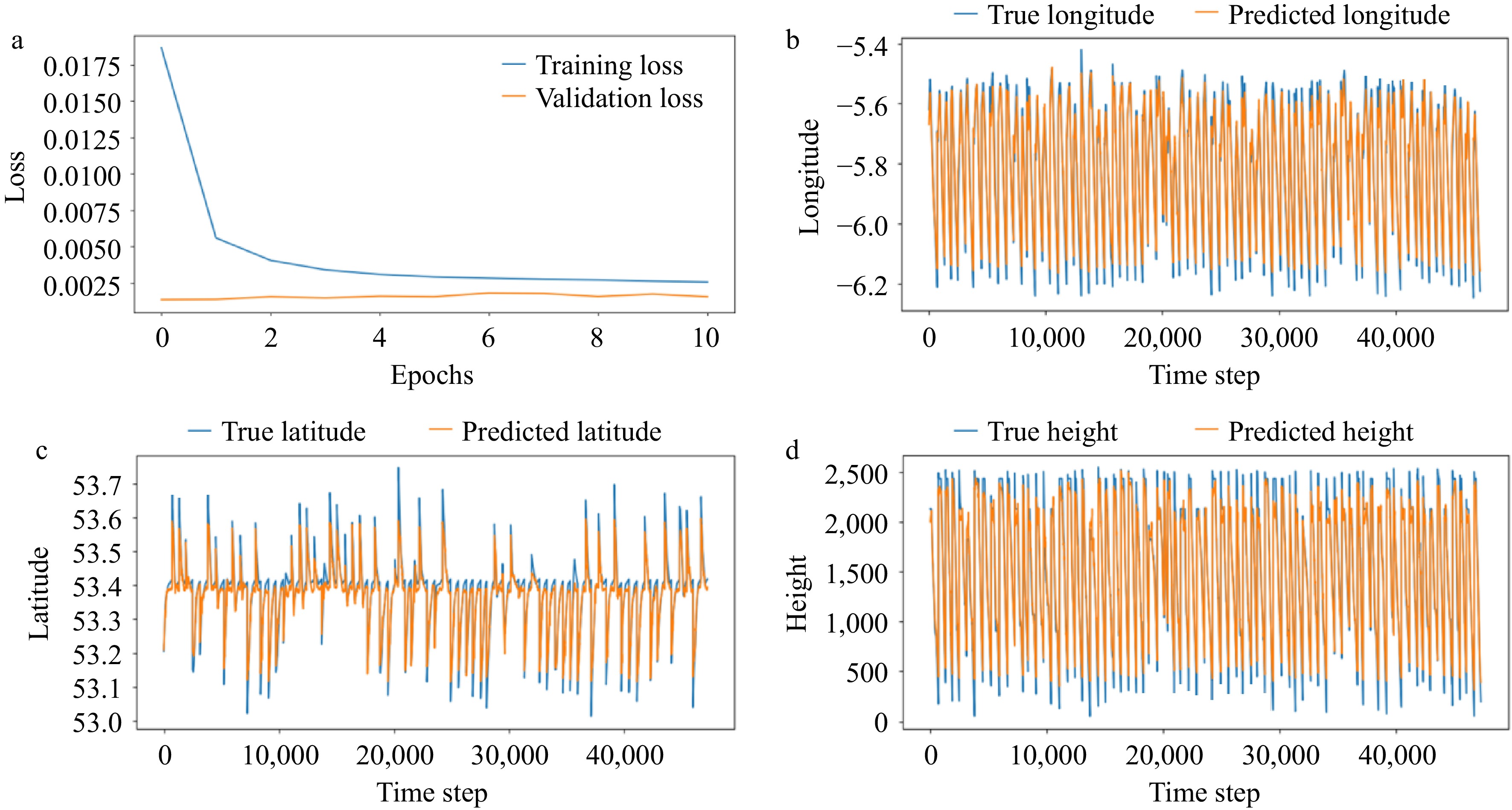
Figure 2. 

(a) CNN loss characteristic curve and CNN model prediction of (b) longitude, (c) latitude, and (d) height based on the CNN model.

Through the validation loss curve, it is found that the validation loss curve rises, and overfitting occurs, indicating that the model 4D trajectory prediction effect of CNN is general. For longitude prediction, the overall trend remains consistent, but the end position prediction has a large deviation, indicating that the prediction of the final result has a large deviation, and the accuracy lacks accuracy. For latitude prediction, the overall trend remains consistent, but the end position prediction has a large deviation, indicating that the final result has a large deviation after prediction, and the accuracy lacks accuracy. For latitude prediction, the overall trend remains consistent, but the end position prediction has a large deviation, indicating a large deviation in the final result of the prediction and a lack of accuracy, and a large error in the prediction occurs when there is a small change in the fluctuation of latitude. For altitude prediction, there is still an inaccuracy in the prediction of the end position, which is followed up by a test on the prediction ability of the LSTM model.

Analysis of LSTM model prediction results

The results of the LSTM model are shown in Table 2.

By observing the results in Table 2, the latitude and longitude predictions are more accurate and significantly better than the CNN model. Height prediction accuracy is lacking, but also significantly better than the CNN model, which shows the superiority of LSTM in handling data of time series. In terms of time, the MAPE results are observed and found to be superior.

The LSTM loss characteristic curves with the LSTM model longitude, latitude, and height predictions are shown in Fig. 3.

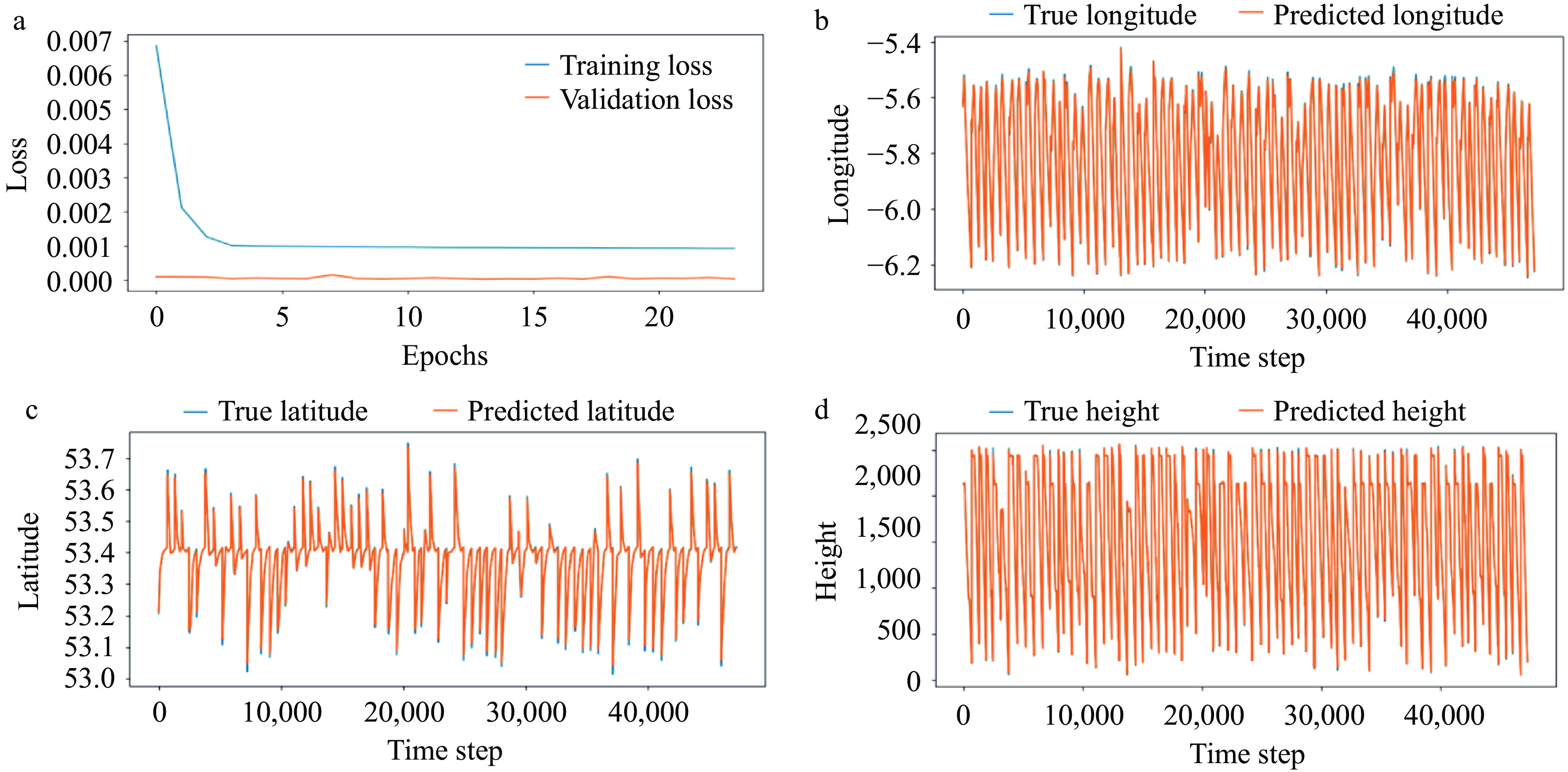
Figure 3. 

LSTM loss characteristic curve and prediction of longitude, latitude, and altitude based on the LSTM model. (a) LTSM loss characteristic curve, LTSM model (b) longitude, (c) latitude, and (d) height prediction and actual illustration.

The training loss decreases rapidly and stabilizes in about three steps, indicating that the LSTM model learns the point merge approximation pattern faster. The subsequent validation loss has no obvious rising trend, indicating that there is no obvious overfitting. The longitude prediction is more accurate, solving the problem of inaccurate CNN prediction of the end point location; the latitude prediction is more accurate, solving the inaccuracy of the end point prediction while also solving the accurate prediction of the latitude under the small fluctuation of the latitude. The actual and predicted values of the altitude are almost overlapped, indicating that the altitude prediction is more accurate.

Comparison of prediction results

According to Tables 1 and 2, it can be seen that the LSTM model outperforms the CNN model in predicting time.

The comparison of prediction results of the two models in horizontal and vertical dimensions, as well as in longitude, latitude, and altitude is shown in Fig. 4.

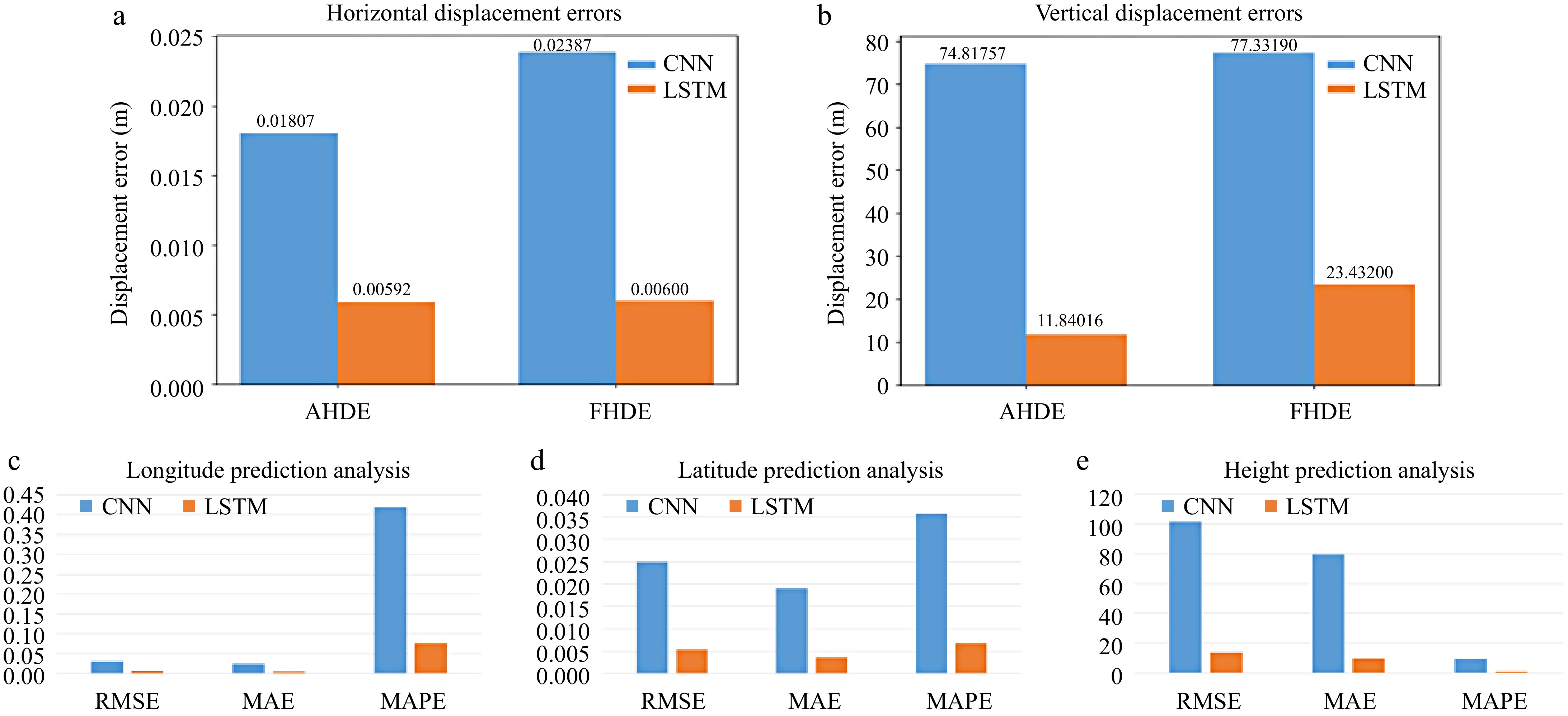
Figure 4. 

Comparison of prediction results. Comparison of prediction results in (a) horizontal dimension and (b) vertical dimension between two models. Comparison of (c) longitude prediction results, (d) latitude prediction results, and (e) height prediction results between two models.

In the horizontal dimension, the LSTM model is significantly better than the CNN model. The displacement error indicators AHDE, FHDE, AHDE, and FHDE of LSTM are all smaller than those of the CNN model; In the vertical dimension, the LSTM model also outperforms the CNN model in predicting values. The displacement error indicators HVDE, FVDE, HVDE, and FVDE of LSTM are all smaller than those of the CNN models.

In terms of longitude, latitude, and altitude prediction, LSTM performs significantly better than CNN models. The RMSE, MAE, and MAPE values of the LSTM model are all lower than those of the CNN model, indicating that it is more accurate in predicting the trajectory of longitude, latitude, and altitude. In summary, the LSTM model with better temporal characteristics is selected as the last model chosen for 3D and 2D plotting and prediction, and it is seen that the prediction results are better, as shown in Fig. 5.

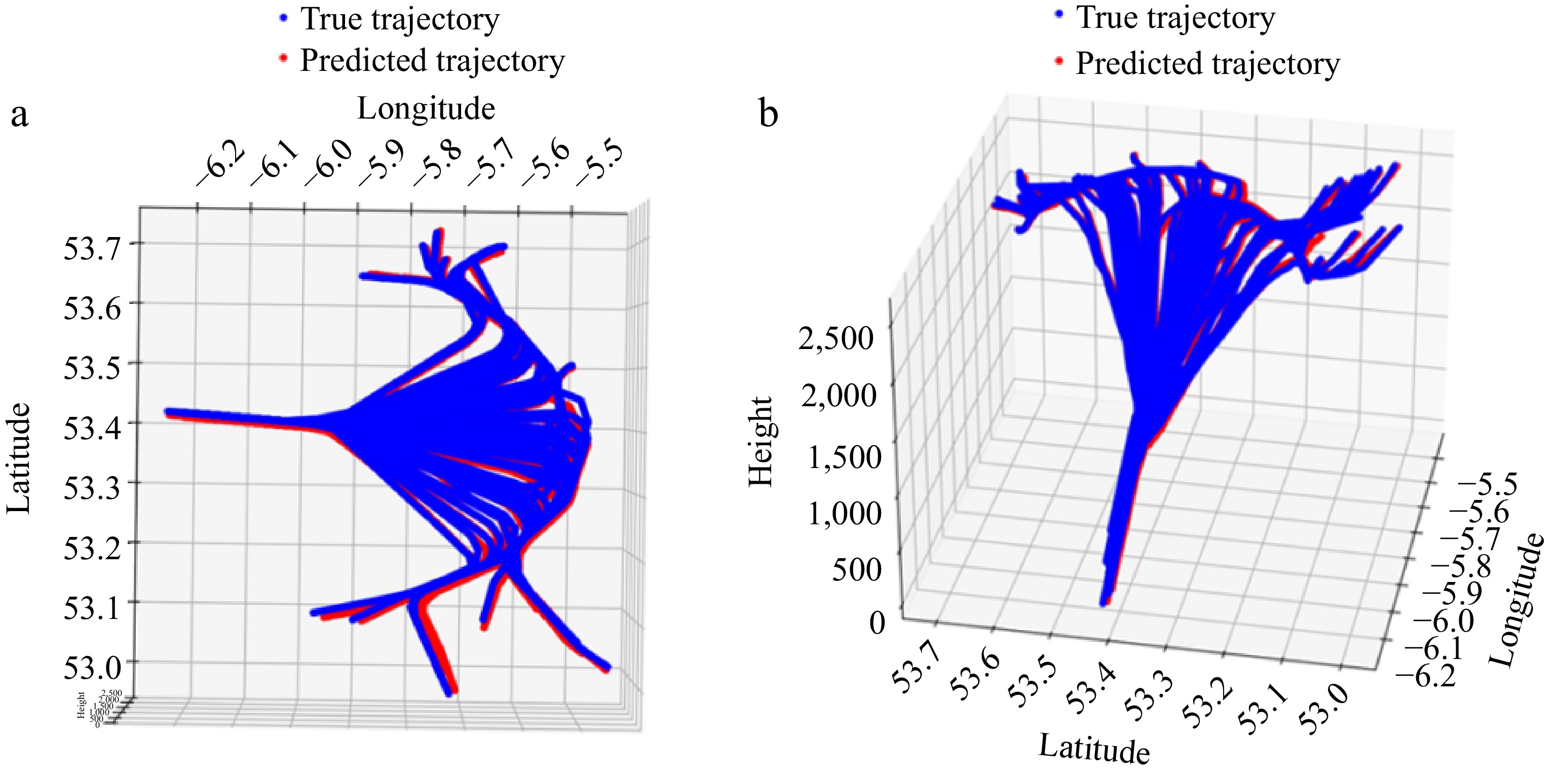
Figure 5. 

(a) 2D and (b) 3D illustration of the LSTM model.

In summary, the LSTM model is significantly better than the CNN model in all aspects and has better prediction results, and it is feasible to use the LSTM model for 4D trajectory prediction. The test set performs better on 3D and 2D illustrations.

In this paper, the research on 4D trajectory prediction methods for aircraft in point merge approach mode is proposed. Through the data preprocessing based on the principle of point merge, the division and screening of route data, and the comparative analysis of the simulation results of the two models, CNN and LSTM, it is shown that the prediction of the LSTM model is significantly better than that of the CNN model in four aspects, namely, time, longitude, latitude, and altitude, and the LSTM model performs excellently in the processing of sequential data, especially in the prediction of longitude and latitude, and the degree of accuracy of its prediction is significantly higher than the CNN model. Although there is some error in height prediction, the overall performance is still better. Through the drawing of 3D and 2D illustrations, it is verified that the LSTM model has high feasibility and prediction accuracy for 4D trajectory prediction in point merge approach mode. Therefore, the LSTM model is selected as the final 4D trajectory prediction model.

Future research work includes improving the prediction capability of the model by collecting more high-quality route data and considering other features such as speed and vertical velocity.