Short-term inbound passenger flow forecasting for urban rail transit based on phase space reconstruction and deep learning

With the acceleration of urbanization, the urban rail transit systems in megacities are becoming increasingly crowded during peak periods, presenting significant challenges in passenger flow management^[1]. Short-term passenger flow forecasting (STPFF) can provide real-time traffic information to assist urban rail transit authorities in managing passenger inflows, optimizing train scheduling, handling emergencies, and helping passengers choose optimal travel times and routes. It plays a crucial role in ensuring the efficiency and safety of urban rail transit. However, due to the complex impacts of factors such as passenger behavior, weather, and unexpected events^[2], passenger flow entering stations exhibits significant nonlinearity and randomness^[3], posing substantial challenges for STPFF. STPFF has attracted widespread attention from researchers due to its practical significance.

In the early stages, traditional statistical methods provided basic forecasting approaches, such as historical data regression analysis^[4], exponential smoothing^[5], and ARIMA models^[6]. These methods rely on fixed model structures and parameters, making it difficult to capture dynamic changes in passenger flow, limiting forecasting accuracy^[7]. With the development of machine learning, models based on machine learning techniques have been introduced for short-term passenger flow forecasting, such as Bayesian Networks^[8], Random Forests (RF)^[9], and Support Vector Machines (SVM)^[10]. These models have some ability to model nonlinear relationships, but they face limitations when considering more complex spatiotemporal correlations^[11].

In recent years, deep learning methods, due to their powerful feature extraction capabilities have been widely applied in the field of STPFF. Long Short-Term Memory (LSTM) networks, with their recurrent structure and parameter-sharing advantages^[12], are suitable for forecasting passenger flow at a single station^[13]. However, the single LSTM model relies on one-dimensional passenger flow time series provided by Automatic Fare Collection (AFC) data, making it difficult to fully capture the nonlinear characteristics of passenger flow. Convolutional neural networks (CNN) and LSTM can be combined to address the limitations of single networks. CNN effectively handle spatial issues^[14], and hybrid models that integrate spatial, variability, and periodic features of passenger flow exhibit better prediction accuracy than baseline models^[15]. However, relying solely on the fusion of spatial and temporal features is inadequate for fully capturing the complex dynamic characteristics of passenger flow under varying external conditions. Emerging research has gradually shifted towards integrating multidimensional influencing factors into hybrid models^[16−20] to further enhance prediction accuracy and model applicability. For instance, hybrid models of Graph Convolutional Networks (GCN) and LSTM that consider station connectivity, weather conditions, and air quality demonstrate high prediction accuracy^[21], but challenges remain in obtaining and processing real-time data, including computation delays and high complexity, making it difficult to meet real-time prediction needs. Additionally, these models often rely on human experience to adjust parameters, which affects their generalization ability and adaptability. In practical applications, balancing prediction accuracy and real-time performance remain a problem that requires resolution.

However, due to the complex impacts of factors such as passenger behavior, weather, and unexpected events^[2], passenger flow entering stations exhibits significant volatility, which becomes increasingly pronounced as the data collection interval is reduced^[22]. It has been demonstrated that short-term passenger flow data typically exhibits nonlinear and chaotic characteristics^[23]. Chaos is the unity of determinism and randomness, simultaneously embodying both global stability and local instability^[24]. In-depth study of chaotic phenomena can help reveal their internally complex yet orderly structure, thereby uncovering the underlying laws behind these seemingly irregular phenomena^[25]. On one hand, chaotic systems are highly sensitive to initial conditions and small disturbances, resulting in long-term unpredictability. On the other hand, although the trajectories may seem to diverge, they are actually confined by strange attractors, allowing for the identification of their underlying patterns and short-term prediction^[26].

According to Taken’s theorem^[27], in chaotic systems, the future state of one dimension depends on interactions with other dimensions. This principle underlies Phase Space Reconstruction (PSR), which reconstructs chaotic attractors in a higher-dimensional space from one-dimensional time series data. PSR reveals the inherent irregularity and self-similarity of the data^[28]. Therefore, PSR serves as a prerequisite for the nonlinear time series analysis and forecasting of data from chaotic systems^[29].

At the same time, short-term passenger flow data often exhibits periodicity, with patterns recurring on a daily or weekly basis. This time-dependent behavior indicates that historical data with similar periodic characteristics can assist in predicting future passenger flows. LSTM networks are particularly well-suited for this task, as they can capture both short-term and long-term temporal dependencies by learning the relationships between past and future values over time. Therefore, a forecasting model that integrates both chaotic features extracted by CNN from the reconstructed phase space and temporal dependencies captured by LSTM is expected to yield more accurate results.

This study proposes a novel forecasting model that combines Phase Space Reconstruction (PSR) with the deep learning model CNN-LSTM. The PSR method is employed to transform the original one-dimensional time series into a multi-dimensional phase space, unveiling the chaotic features inherent in the dynamical system. The CNN-LSTM model is utilized to learn both spatial features (phase space features) and temporal features of the passenger flow data. The model's hyperparameters are optimized using the Grey Wolf Optimizer (GWO), further enhancing its performance. Experimental results demonstrate that, compared to single models and other advanced hybrid models, the PSR-CNN-LSTM model exhibits significant advantages in prediction performance, convergence speed, and stability. It effectively uncovers passenger flow patterns in short-term nonlinear and chaotic AFC transaction data, enabling accurate forecasting of short-term station passenger flow.

The contributions and highlights of the study are as follows:

(1) By calculating the Lyapunov exponent of the passenger flow time series, the chaotic characteristics were quantitatively identified.

(2) Using a Phase Space Reconstruction method to expand the one-dimensional passenger flow time series into a high-dimensional space, enabling accurate capture of passenger flow volatility while significantly reducing data complexity.

(3) The integration of CNN and LSTM enables comprehensive capture of spatiotemporal features in phase space. CNN effectively extracts spatial features from the reconstructed high-dimensional phase space data, while LSTM handles temporal dependencies within the time series based on phase space features.

(4) The GWO algorithm optimizes the proposed forecasting model's parameters automatically, adapting the model to varying data in different situations, and maintaining stable prediction performance under various uncertainties and dynamic changes.

The dataset used in this study was sourced from the Automated Fare Collection (AFC) system of the Shanghai Metro Line 1 and Line 2, covering passenger entry and exit transactions from April 1 to April 30, 2015. The raw dataset contained non-rail transit records (e.g., bus transactions) and redundant attributes such as fare type classifications, which were filtered and cleaned to ensure relevance to subway passenger flow analysis. The original data format is summarized in Table 1.

The specific steps for data preprocessing are as follows:

(1) Data cleaning: Non-rail transit records (e.g., bus transactions) and irrelevant attributes (e.g., fare type information) were systematically removed. Additionally, records logged during non-operational hours (23:30–05:30) were excluded, as these periods lack passenger activity and do not contribute to meaningful forecasting. Duplicate entries with identical timestamps and station identifiers were also identified and removed.

(2) Outlier handling: Statistical thresholds were applied to detect anomalies in passenger counts. Values exceeding three standard deviations (Z-score > 3) or displaying negative entries were flagged as outliers. These anomalies were replaced via linear interpolation using adjacent time intervals to preserve temporal continuity. Negative values, indicative of data corruption, were directly discarded.

(3) Identification of entry and exit records: Since the original data did not distinguish between entry and exit records, this study determined the entry and exit status based on the fare deduction amount. Records with a fare deduction of 0 were labeled as entry, while non-zero values indicated exit. This rule was validated against station layouts to ensure consistency.

(4) Time granularity classification: To facilitate short-term passenger flow forecasting, the processed data was aggregated into non-overlapping 10-min intervals using time-series resampling techniques.

After the above preprocessing steps, the data was integrated into records of passenger entries for each station, grouped by different time intervals, as shown in Table 2.

The processed entry passenger flow data about each station can be regarded as a set of one-dimensional time series obtained within specific collection intervals. In the temporal dimension, the one-dimensional time series of entry passenger flow at a station is represented as,

where, $f_t^s$ represents the entry passenger flow at the station during the t-th time interval.

Chaos identification

The application of phase space reconstruction to prediction is based on the premise that the time series exhibits chaotic characteristics^[30]. To visually demonstrate the significant fluctuations in inbound passenger flow over time, data from a station is plotted over 20 working days, as shown in Fig. 1. The figure shows that the fluctuations do not follow a simple linear pattern but exhibit significant randomness and complexity, indicating strong nonlinear characteristics. The absence of sinusoidal patterns serves as a key characteristic of chaotic signals.

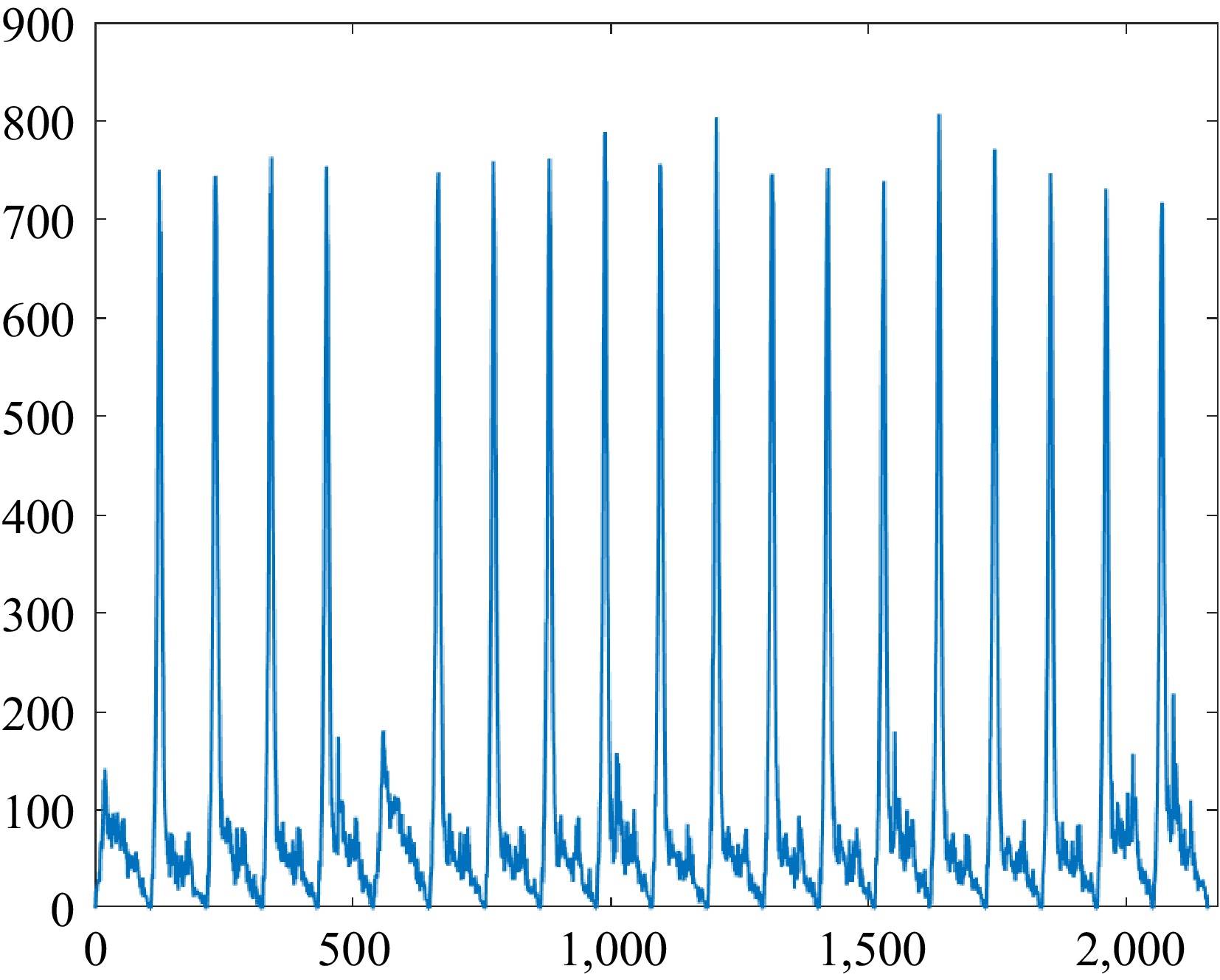
Figure 1. 

Inbound passenger flow variation.

To obtain a more accurate assessment, we further conduct quantitative analysis by calculating the Lyapunov exponent. The Lyapunov exponent precisely characterizes the dynamic convergence or divergence trend of adjacent trajectories in phase space over time^[31]. A positive value indicates that the system exhibits chaotic behavior, while a zero or negative value suggests that the system tends toward randomness or periodicity.

Wolf's method^[32] was used to calculate the maximum Lyapunov exponents (MLEs). The formula is,

where, L_i represents the distance between two neighboring points in phase space reconstruction, $L_i^\prime $ represents the distance between two points at the next moment, and M is the total number of iterations.

In this study, MLEs solely for identifying chaos and do not influence the subsequent forecasting or prediction steps. The chaotic characteristics of passenger flow at metro stations exhibit significant spatial heterogeneity, requiring independent chaos validation for each station. A uniform exponent across stations could obscure these differences and impact the chaos identification process. Therefore, station-specific MLEs are necessary to accurately capture the unique chaotic characteristics at each station. The MLES for various stations on Shanghai Metro Line 1 are calculated and tabulated in Table 3.

All of the values are larger than 0, indicating that the inbound passenger flow at these stations has various varying degrees of chaotic characteristics. The passenger flow time series are reconstructed to the high-dimension in the phase space is feasible.

PSR-CNN-LSTM structure

Since it is difficult to extract representative nonlinear features from one-dimensional passenger flow time series data, PSR of chaotic time series is performed as a preprocessing step before building and training the prediction model. PSR maps the time series into a higher-dimensional phase space, revealing complex nonlinear patterns and temporal dependencies that are not apparent in the original data. This enriched representation provides the model with more informative features, improving its ability to capture dynamic behavior. The reconstructed phase space offers a clear, structured feature set that is then fed into the CNN-LSTM network, which learns from the enhanced features to make more accurate predictions.

Using PSR before training the neural network, rather than as a learnable module within the network, helps maintain training stability and reduces model complexity, while enhancing prediction accuracy and keeping the network more efficient. The PSR-CNN-LSTM structure is illustrated in Fig. 2.

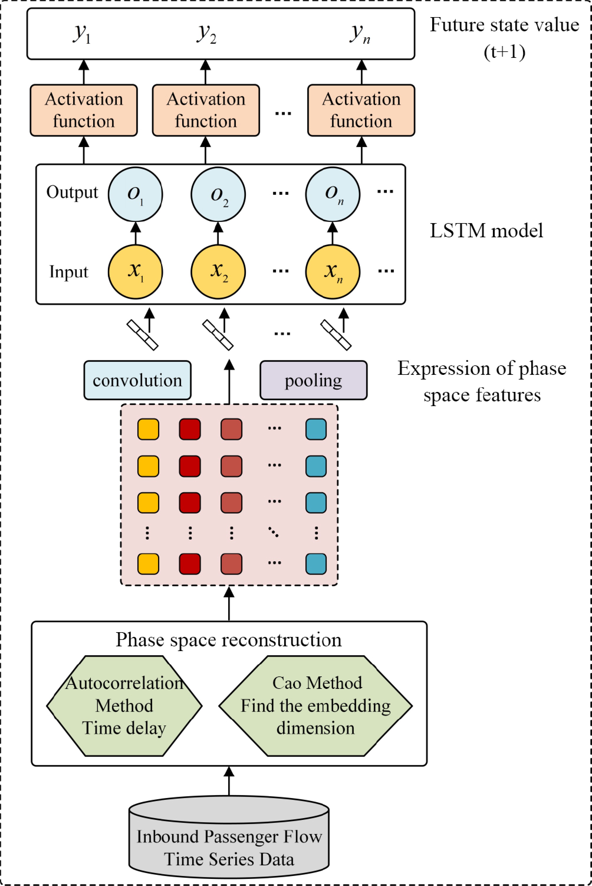
Figure 2. 

Structure of the PSR-CNN-LSTM model.

Phase space reconstruction

To restore its original space, the phase space is reconstructed with the coordinate delay reconstruction method^[33−35]. The dataset of the reconstructed chaotic time series can be represented as the phase space domain Y and the chaotic time series X. The process of phase space reconstruction is illustrated in Fig. 3.

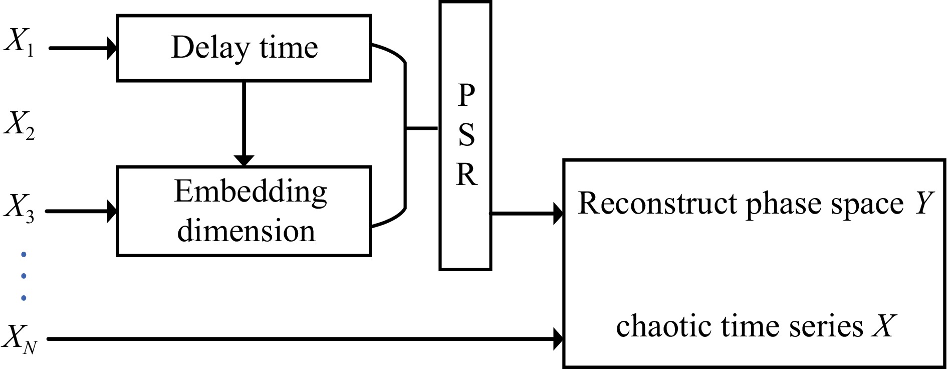
Figure 3. 

The process of phase space reconstruction.

This involves embedding the one-dimensional time series data {x_i | i = 1, 2, ···, N} into a higher m-dimensional space including a series of phase points y. Every point in the phase space corresponds to a possible state within the dynamical system. Reconstruct phase space domain Y can be represented as:

where, $\tau $ represents the time lag, and m is the embedding dimension.

To ensure that the phase space can retransfer the original properties, the embedding dimension m has to satisfy:

Through the phase space reconstruction, the morphology and structure of the attractor will emerge, and a mapping function will be obtained F : Hm → Hm, which satisfy:

where, l represents the prediction step, which can be determined based on the reconstructed state variables.

The phase space is used to predict the state of the time series X_n+l, i.e., the next l steps. We use the autocorrelation function method and the Cao method to compute delay time and embedding dimension, respectively.

Determining the delay time

Using the autocorrelation function, the correlation within the time series is extracted, and an appropriate τ value is selected based on the resulting graph. Given a time series x with a sample size of n, a mean value of μ, and a demeaned value of h(i), after td iterations, the autocorrelation function C(τ) can be expressed as,

Based on the autocorrelation function, a curve about the autocorrelation coefficient with the delay time is obtained. In Fig. 4, the autocorrelation function is with the delay time varying. When the value of the autocorrelation function reaches $1 - \dfrac{1}{e}$ 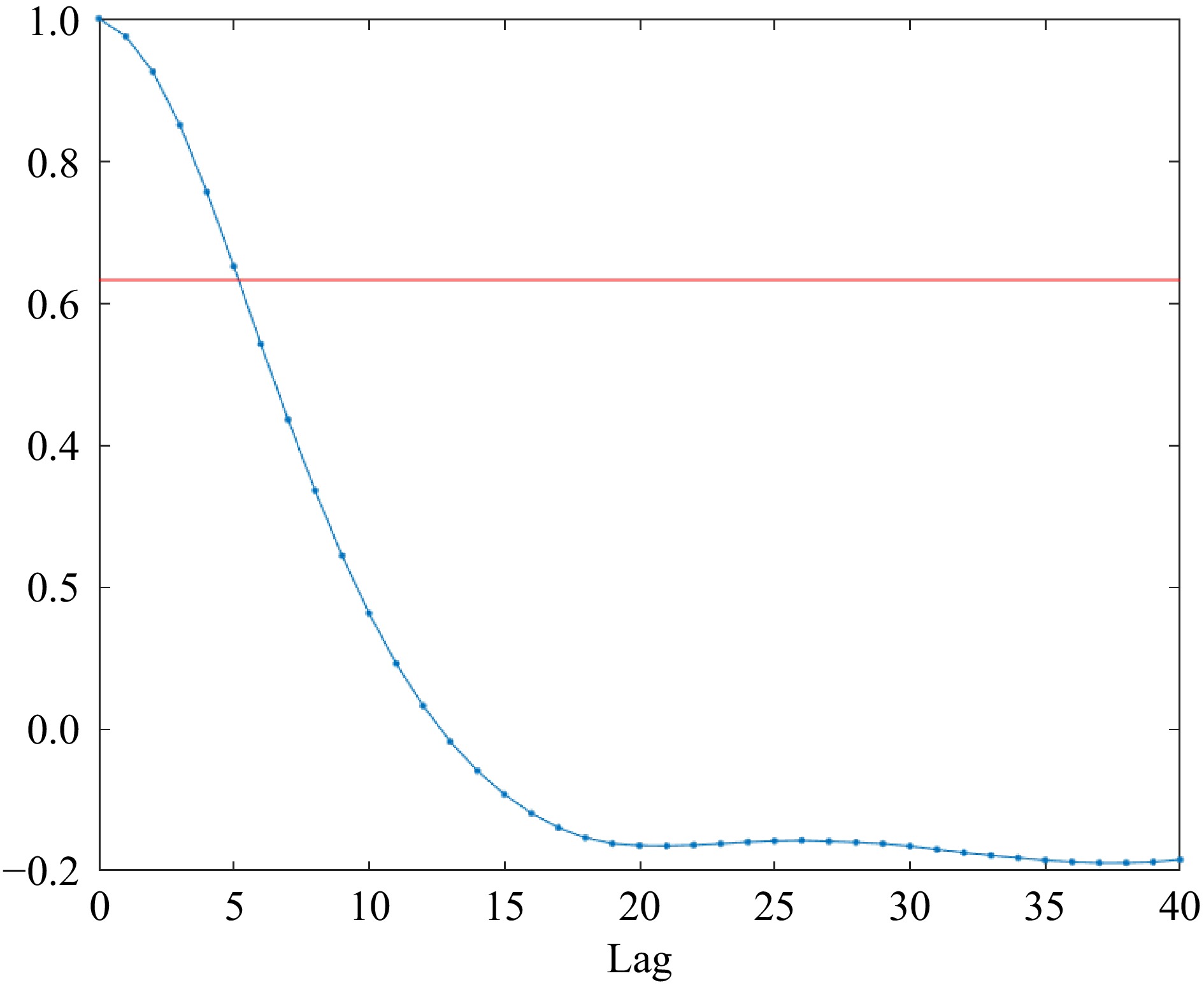times its initial value, the corresponding horizontal coordinate value is 6, which is the optimal delay time.

Figure 4. 

Autocorrelation coefficient.

Determining the embedding dimension

The dominant determining the embedding dimension $ \mathrm{m} $ techniques include the False Nearest Neighbors (FNN) algorithm, the Grassberger-Procaccia (G-P) method, and the Cao method^[36]. Reducing the dependence on the prefined threshold, the Cao method can more accurately capture the intrinsic structure of complex data during processing and is presented as,

where, X_i(m+1) represents the i-th vector in the phase space, and X_n(i,m)(m) is the vector closest to X_i(m+1).

The mean value of all α(i,m) is defined as,

Let E₁(m) = E(m+1)/E(m), when m > m₀ and E(m) is no longer changing, the embedding dimension is m₀+1 and the optimal. The curve of embedding dimension variation is plotted in Fig. 5. When m = 28, E₁(m) no longer changes, indicating that the minimum embedding dimension is 28.

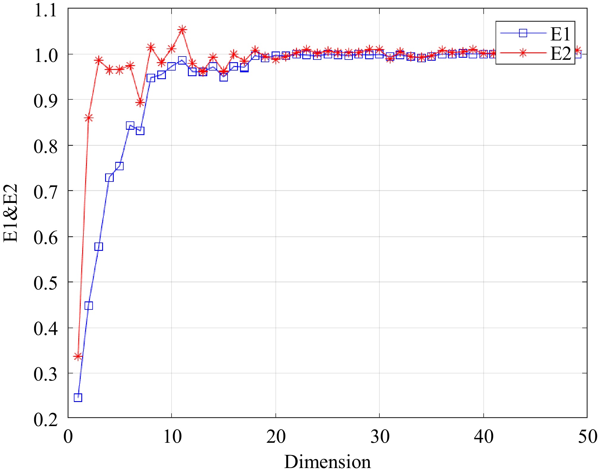
Figure 5. 

Embedding dimension.

Based on the embedding dimension m = 28 and the delay time τ = 28, we deduce the number of phase points M = N − (m − 1)τ. Equation (9) represents the resulting phase space matrix:

Each column in the dataset represents a sample, with a total of 1,998 samples. Each sample has 27 feature values and one response value. Then the order of the data is shuffled to improve the generalization ability of the model.

Phase space visualization

The phase diagram obtained by reconstructing the passenger flow data with different delay times is shown in Fig. 6.

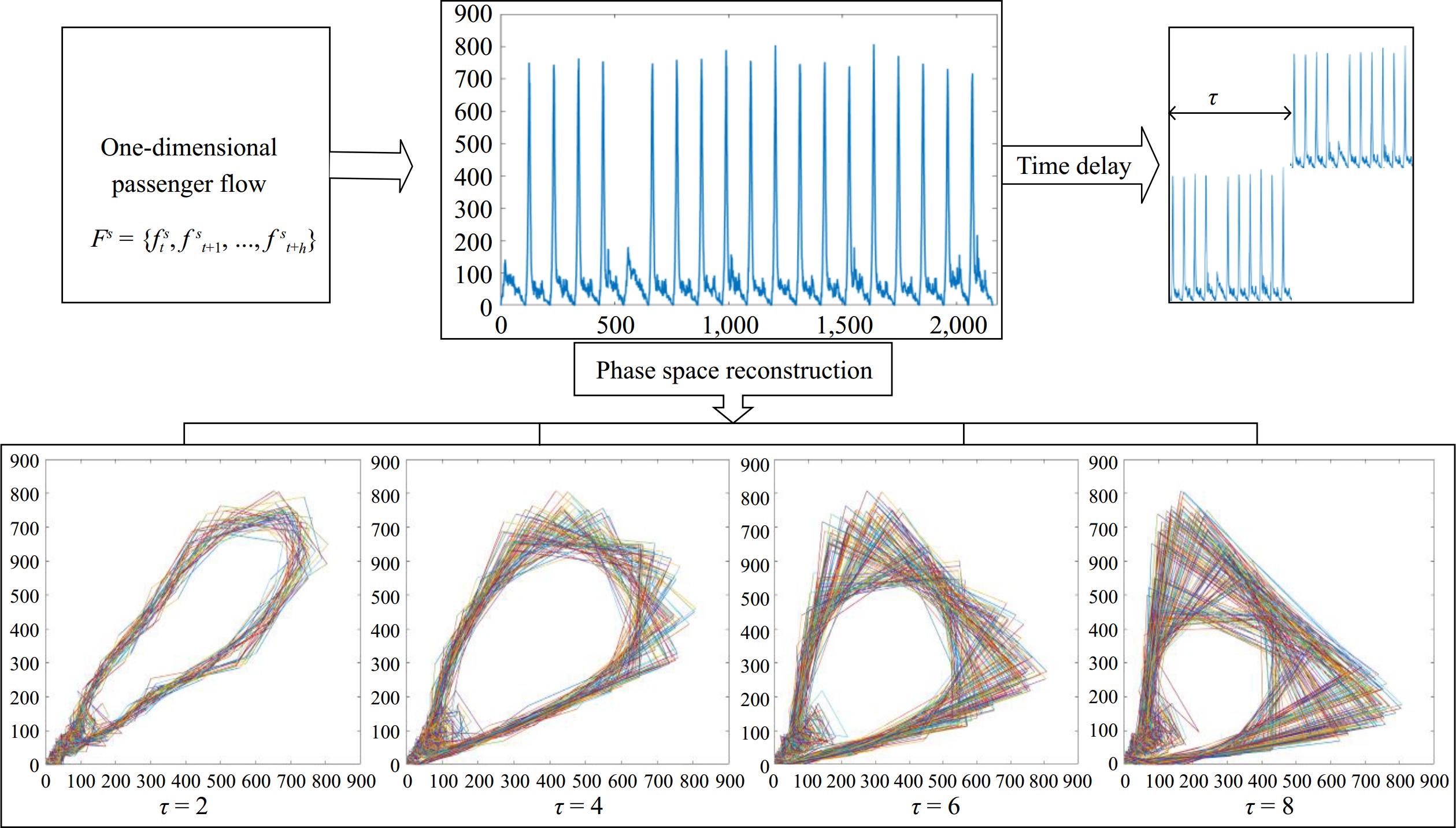
Figure 6. 

Phase space at different delay times.

From the phase space plot of the passenger flow time series shown in Fig. 6, we observe multiple folding of the trajectories, which intertwine to form a tightly interlaced image pattern. Based on this observation, we can conclude that there exists a unique dynamic structure within the system, known as a strange attractor. This finding further supports our inference that the passenger flow time series exhibits chaotic characteristics.

It can also be observed that selecting an appropriate delay time helps in better extracting the nonlinear features of the system. When the value of the delay time is too large, it becomes difficult for the system to accurately capture the dynamics of the original sequence. This causes the originally simple orbit to become overly complex and reduces the number of valid data points. Conversely, if the delay time is too small, the reconstructed phase orbits will become tightly clustered along the diagonal due to a strong correlation, preventing the effective demonstration of the system's dynamic characteristics.

CNN-LSTM model

After being transformed into a two-dimensional pattern through phase space reconstruction, this two-dimensional matrix is fed into the CNN component, where it undergoes two convolutional layers to extract high-dimensional feature information. The pooling layer then filters out the critical features, and the Flatten layer flattens the input data, outputting a one-dimensional vector with high-dimensional feature information. Finally, this vector is input into the LSTM to extract temporal features, leveraging its temporal memory capabilities to deeply integrate and precisely extract the features output by the CNN, thereby predicting the future state values of passenger flow. The structure of CNN-LSTM is shown in Fig. 7.

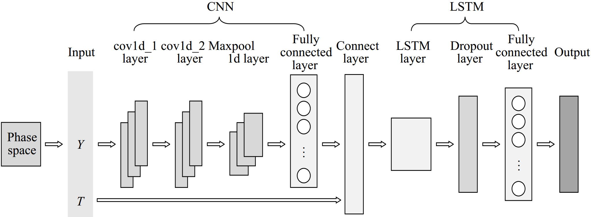
Figure 7. 

CNN-LSTM structure.

CNN capturing spatial features of passenger flow

The two-dimensional matrix reconstructed in the phase space is inputted in the CNN network, whose size is [n − (m_i − 1)τ_i, m]. In the matrix, each row denotes a phase space point with a length of the embedding dimension m, the length of the column corresponds to that of the time series. In the CNN network, the high-dimensional features of the time series are extracted to capture the local features and the patterns in the sequence with the convolutional function H(x) as,

where, f(·) and g(·) are integrable functions, respectively; x and u are variables.

In the 1D CNN network, the temporal patterns passenger flow is treated as image channels, considering the 1D time series data as a special form of image where time steps equate to image pixels. We discuss the two-dimensional passenger flow time series reconstructed in the phase space, which are ‘image-like’ data. Through this approach, the spatial features captured by CNN in the passenger flow phase space include:

(1) Local dynamics patterns, the dynamic characteristics of the original 1D passenger flow time series are mapped into a new phase space, which deduces the dynamic and behavior features of similar systems.

(2) Hierarchical structures, denoting the various scale dynamic patterns learned by the CNN network ranging from the shorter, local dynamic patterns to the longer, more complex ones.

(3) Invariant features, and similar dynamic patterns will be captured by the CNN network, regardless of transformations such as translation, and rotation of the input data, which is particularly important to deal with complex data in the phase space.

LSTM capturing temporal features about the passenger flow

By introducing the forget gate, input gate, and output gate, the issues of gradient vanishing and explosion in Recurrent Neural Networks (RNN) can be effectively addressed. The structure is shown in Fig. 8.

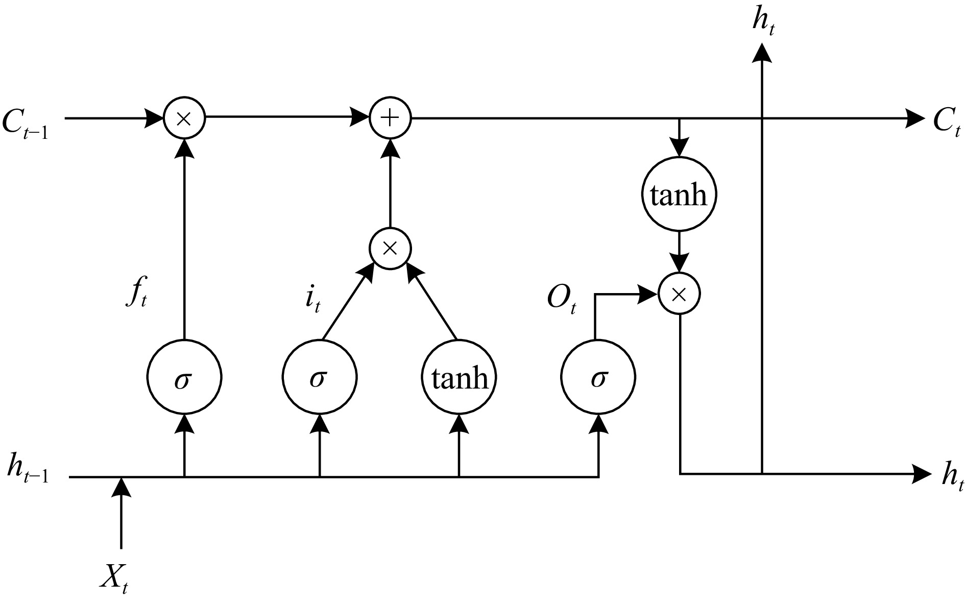
Figure 8. 

LSTM internal structure diagram.

The forget gate determines the importance of past memory cells, deciding whether to retain the previous memory unit based on the current input unit X_t and the previous output unit h_t−1. The input gate controls whether the memory unit value at time t should be used to update the memory unit value at the next time step. The output gate distinguishes between memory cells and hidden layer units, thereby updating the hidden state. The update equation for LSTM is as follows:

where, σ represents the sigmoid function, tanh is the nonlinear activation function, W is the weight matrix for each gate, and b is the bias term for each gate.

The long-term dependencies and more complex temporal features of the time series are captured with the LSTM network. Based on the captured long-term dependencies about the passenger flow sequence, the future passenger flow will be predicted with the subsequent fully connected layers.

Thus, combining CNN and LSTM models, two primary features in time series are captured:

(1) Local temporal features: Short-term time dependencies extracted by the CNN, such as short-term fluctuations or periodic patterns in the time series, allowing for consideration of dynamic changes at the current moment during prediction.

(2) Global temporal features: Long-term time dependencies extracted by the LSTM, which may span multiple time steps and reflect the overall trend or structure of the time series, enabling consideration of dynamic changes over a longer time horizon during prediction.

Hyperparameter optimization

To improve the model's adaptability to varying input data and environmental conditions, adaptive parameter adjustment is necessary. The GWO algorithm^[37] has a simple structure, is easy to implement, and offers strong global search capabilities. It outperforms PSO and GA in terms of convergence speed and accuracy^[38]. Salp Swarm Algorithm (SSA)^[39], a recently emerged nature-inspired optimization technique, has been shown to effectively optimize CNN-LSTM networks with higher prediction accuracy than PSO and other algorithms. We employ GWO as the primary optimization algorithm and incorporate the SSA, which shares similar principles, into the ablation study to facilitate a direct comparison with GWO in optimizing the hyperparameters of the PSR-CNN-LSTM model.

Grey Wolf Optimization algorithm

The fitness function used for minimization using GWO is mean square error is,

where, f is a fitness function used in GWO, Y_true is the test data used to compare with predicted data, and Y_pred is the predicted data from trained model.

The features are evaluated with the best combination of hyperparameters by minimizing the fitness function^[40].

The algorithm flow is as follows:

(1) Initiate GWO Optimization Process: The position parameters of the Alpha, Beta, and Delta wolves are updated by calculating the fitness values, thereby gradually optimizing the parameters of the neural network.

(2) Extract Optimal Results: After the optimization process concludes, the optimal learning rate, the optimal number of convolutional kernels, and the optimal number of neurons in the hidden layer are extracted from the final position parameters. These parameters will be used to construct the final CNN-LSTM model.

By removing the subjective biases associated with manual adjustments, it ensures consistent and objective performance. The integration of the hyperparameter optimization algorithm enhances the model's stability and generalization ability, allowing it to self-adjust to new datasets without the need for re-tuning. This not only improves performance but also reduces time and computational costs, making the model more efficient and suitable for large-scale applications across multiple stations and diverse environments.

Data from the first three weeks were used to predict inbound traffic for the last week. The number of input features is equal to the dimension of the reconstructed phase space, while the number of output features is 1. The specific parameters are shown in Table 4. The total number of iterations for the model is determined through experimental validation beforehand and is ultimately set to 100 rounds, 1,400 iterations.

Evaluation metrics

To comprehensively evaluate the performance of the short-term passenger inflow forecasting model, we select Root Mean Square Error (RMSE), Mean Absolute Error (MAE), and the Coefficient of Determination (R²) as the evaluation metrics for the prediction effectiveness of the model. These metrics measure the differences between the predicted values and the actual values from different angles, as calculated by Eqs (17)−(19). A larger RMSE and MAE indicates a higher error of the model, whereas a higher R² indicates a better model fit.

Time granularity selection

In this study, we evaluate three commonly used time granularities—10 min, 20 min, and 30 min—for predicting the inbound passenger flow on Shanghai Metro. The 10-min granularity is chosen as the smallest time granularity because the AFC system used in the experiment records data every 10 min. This is standard practice for most AFC systems, making 10 min the most appropriate choice for capturing short-term dynamics in passenger flow. The prediction results for these granularities are shown in Table 5.

As shown in Table 5, the prediction accuracy declines with coarser granularities. Specifically, as the granularity increases from 10 to 30 min, RMSE and MAE increase, while R² decreases. This indicates that coarser granularities lead to lower prediction accuracy, primarily because they lose the ability to capture high-frequency fluctuations in passenger flow, which are essential for short-term forecasts.

Since the AFC system provides individual entry records, the time granularity (e.g., 10-min, 20-min, or 30-min intervals) is determined during the data preprocessing stage. Coarser granularities, such as 30-min intervals, may reduce the model's ability to capture short-term fluctuations, which can affect prediction accuracy. However, this issue can be mitigated during preprocessing by aggregating the data into the desired granularity. For instance, resampling individual entry records into 10-min intervals helps retain detailed temporal patterns, improving model performance.

At the same time, the PSR-CNN-LSTM model is flexible and does not require structural changes to handle different granularities. If there is a delay in real-time data, the model can still operate effectively, maintaining similar performance without modifying its core architecture, regardless of whether the data is aggregated into 10-min, 20-min, or 30-min intervals.

Prediction performance of the PSR-CNN-LSTM

To evaluate the generalization capability of the PSR-CNN-LSTM model, we applied it to five representative stations in Shanghai, each located in different functional regions with distinct passenger flow patterns. The results for these stations are shown in Fig. 9.

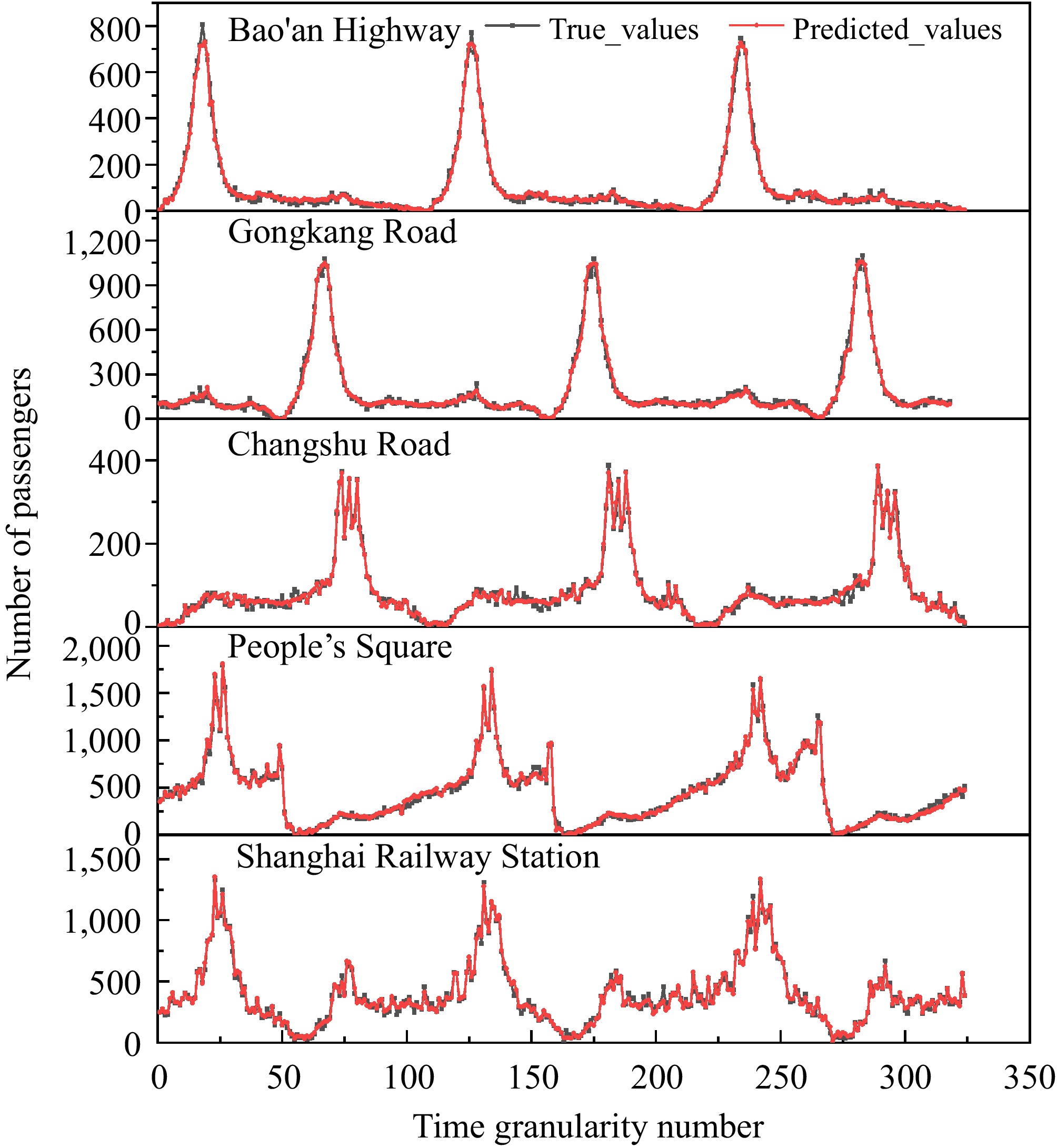
Figure 9. 

Prediction of passenger flow for typical stations of the Shanghai metro.

(1) Bao'an Highway Station (Suburban Residential Area): This station primarily serves residential commuters during peak hours. The model predicts passenger flow with high accuracy, particularly during peak times, with predicted and actual flows closely matching.

(2) Gongkang Road Station (Mixed-Use Community): Located in a mixed residential and commercial area, this station experiences more complex flow dynamics. The model accurately captures these patterns, showing good prediction accuracy for both peak and off-peak hours.

(3) Changshu Road Station (Tourist Area and Small Transfer Hub): This station has a highly fluctuating passenger flow, especially during tourist seasons and transfer times. Despite the irregularity, the model captures these fluctuations successfully.

(4) People’s Square Station (Major Transfer Hub): With its dual-peak flow pattern caused by commuter and tourist congestion, this complex transfer station’s flow is predicted accurately, demonstrating the model’s ability to handle multi-modal passenger traffic.

(5) Shanghai Railway Station (Transportation Hub): The flow at this station is highly irregular and influenced by train schedules. Despite the randomness, the model captures these fluctuations effectively, proving its robustness in unpredictable environments.

These results confirm that the PSR-CNN-LSTM model demonstrates strong generalization across diverse station types and functional areas within the Shanghai Metro system, consistently delivering accurate predictions in suburban, mixed-use, tourist, and transportation hub settings. This robustness suggests its potential adaptability to other urban transit networks.

Comparison of the performance of different models

Benchmark models and experimental setup

To thoroughly assess the performance of the proposed PSR-CNN-LSTM model, five benchmark models were selected for comparison, representing both classical, and state-of-the-art hybrid approaches:

(1) CNN: A baseline 1D convolutional neural network with two convolutional layers (32 and 64 filters, kernel size 3 × 3), capturing local temporal patterns in raw time series.

(2) LSTM: A standard LSTM network with two hidden layers (200 neurons per layer), serving as a temporal baseline.

(3) CNN-LSTM: A hybrid model combining CNN (32 and 64 filters) and LSTM (200 neurons), directly processing raw time series without phase space reconstruction.

(4) GCN-GRU^[19]: A graph-based model using GCN and GRU to capture network topology and temporal dynamics.

(5) ResNet-LSTM-GCN^[21]: An advanced hybrid model integrating ResNet for spatial correlation, GCN for network topology, and attention-LSTM for temporal dependencies, requiring auxiliary data (e.g., weather, station connectivity).

(6) The experimental results are summarized in Table 6. To provide a clearer understanding of these results, Fig. 10 visually compares the performance of the models.

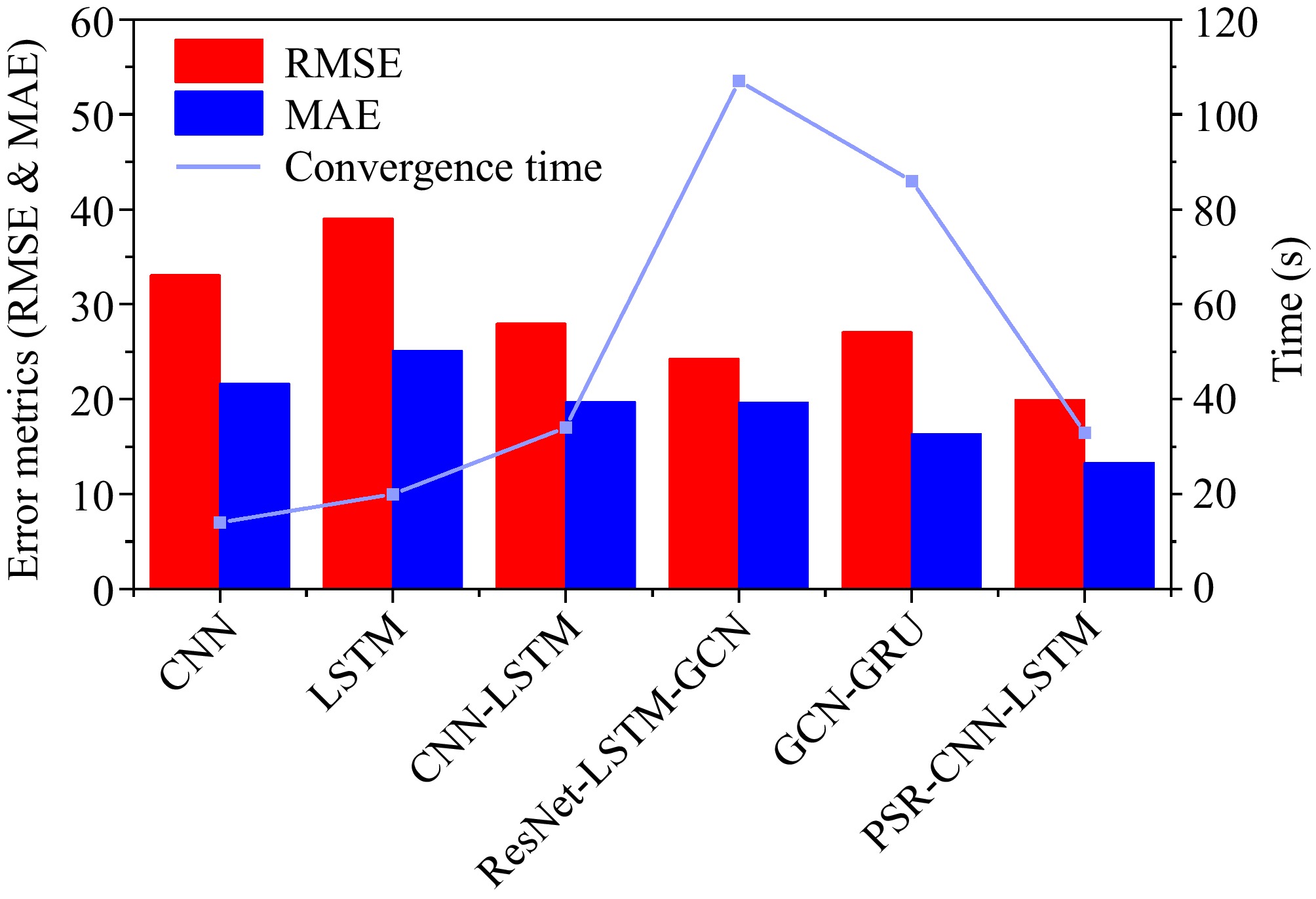
Figure 10. 

Comparison of error metrics and convergence time for models.

The PSR-CNN-LSTM model demonstrates superior predictive accuracy, achieving the lowest RMSE (19.93) and MAE (13.31), and the highest R² (0.99), which emphasizes its effectiveness in forecasting passenger flow. This performance is especially notable when compared to other models in the experiment.

While the CNN and LSTM models focus on spatial and temporal feature extraction, respectively, they fail to effectively integrate both aspects, leading to suboptimal performance in predicting highly complex passenger flow patterns. In contrast, the hybrid CNN-LSTM model combines these two approaches, leading to improved performance. However, the PSR-CNN-LSTM model further enhances feature extraction by incorporating Phase Space Reconstruction (PSR), which significantly improves prediction accuracy. Compared to CNN-LSTM, the PSR-CNN-LSTM reduces RMSE by 28.6% and MAE by 25.8%, demonstrating the critical role of PSR in capturing complex patterns in chaotic time series data.

Although the ResNet-LSTM-GCN and GCN-GRU models exhibit competitive performance, their reliance on auxiliary data (e.g., weather, station connectivity) introduces increased complexity and computational delays. These models take more than 1 min to converge, whereas the PSR-CNN-LSTM model achieves convergence in just 33 s, underscoring its real-time efficiency.

Moreover, PSR-CNN-LSTM operates efficiently with only one-dimensional passenger flow data, reducing the dependency on external factors while maintaining predictive accuracy. This data-efficient approach offers scalability and practical applicability in real-time forecasting for urban rail transit systems. The enhanced performance of PSR-CNN-LSTM can be attributed to its advanced abstraction capabilities via PSR, which effectively captures the dynamic features of passenger flow data, improving both accuracy and generalization.

Thus, PSR-CNN-LSTM not only provides superior performance but also offers an efficient solution for forecasting passenger flow in complex environments, making it an ideal model for real-time prediction in urban rail transit systems.

Ablation study

To validate the effectiveness of each component in the PSR-CNN-LSTM model, we conducted ablation studies by systematically modifying the model's structure and optimization techniques:

(1) PSR-CNN: Removed the LSTM layer and replaced it with a fully connected layer to assess the necessity of temporal modeling.

(2) PSR-LSTM: Removed the CNN layers to evaluate the contribution of spatial feature extraction.

(3) CNN-LSTM (GWO): Removed the PSR layers to evaluate the contribution of PSR.

(4) PSR-CNN-LSTM (SSA): Replaced GWO with the Salp Swarm Algorithm (SSA) for hyperparameter optimization to compare the effectiveness of different optimization methods.

(5) PSR-CNN-LSTM: Removed the hyperparameter optimization component to evaluate the baseline model performance without optimization.

The results of the ablation study, as summarized in Table 7, reveal the crucial role each component plays in the PSR-CNN-LSTM framework. For a more intuitive comparison, Fig. 11 provides a visual representation of these results.

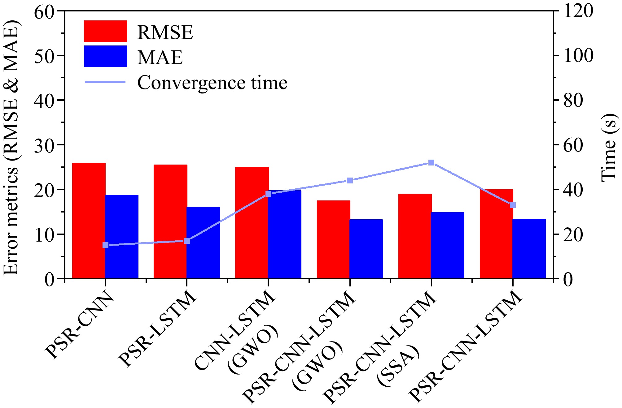
Figure 11. 

Error metrics and convergence time comparison.

The PSR-CNN variant exhibits a performance drop, highlighting the role of LSTM in capturing long-term dependencies in dynamic systems. Similarly, the reduced accuracy in PSR-LSTM emphasizes the contribution of CNN in extracting high-dimensional features from the reconstructed phase space.

The analysis also confirms that incorporating PSR significantly enhances prediction accuracy. In particular, the RMSE is reduced by 40.4%, demonstrating the importance of phase space reconstruction in capturing the underlying structure of non-linear and stochastic systems.

Moreover, when comparing GWO with SSA for hyperparameter optimization, GWO achieves comparable accuracy while using 65.6% fewer parameters. This significant reduction in parameter count makes GWO a more efficient choice, particularly for real-time applications where computational resources are often constrained.

The GWO-optimized PSR-CNN-LSTM model achieves the highest prediction accuracy, as reflected by the lowest RMSE and MAE among all models. However, this enhanced performance comes with a trade-off in terms of both model size, requiring 15% more parameters than the non-optimized model, and convergence time, which is longer compared to the non-optimized version. In real-time scheduling scenarios, omitting the GWO optimization might offer a better balance between computational efficiency, convergence speed, and predictive accuracy. However, in cases where high accuracy is prioritized, but real-time requirements are less stringent and resources are sufficient, the GWO optimization can be used to achieve the best performance. This flexibility allows the framework to prioritize either accuracy or efficiency, depending on the specific operational needs.

To further enhance the applicability, robustness, and computational efficiency of the PSR-CNN-LSTM model, this section discusses its potential for generalization to other transit systems, its adaptability to extreme scenarios, and strategies for improving computational efficiency in large-scale applications.

(1) Expanding Applicability to Other Cities and Transit Systems

The model’s strong generalization across different station types in the Shanghai Metro system suggests its potential applicability to other urban transit networks. While the CNN-LSTM architecture and PSR framework remain applicable, future studies should validate the model in different metro systems to assess whether regional variations in passenger behavior, network structure, and operational policies impact predictive performance.

Moreover, its reliance on AFC entry data makes it adaptable to bus-metro transfer networks, requiring only minor modifications to incorporate multi-modal passenger flows.

(2) Future Work on Extreme Scenarios

Although the model performs well under normal conditions, it requires further enhancements to handle extreme events such as accidents, public events, or weather disruptions, which can cause sudden fluctuations in passenger flow.

To improve adaptability, anomaly detection mechanisms can be integrated directly into the forecasting pipeline. A LSTM-Autoencoder (LSTM-AE) can learn normal passenger flow patterns and detect anomalies based on reconstruction errors, allowing the forecasting model to dynamically adjust predictions in response to unexpected disruptions.

Additionally, incorporating real-time external data (e.g., weather conditions, social media activity, and transit incident reports) could further enhance the model’s accuracy under extreme conditions.

(3) Future Work on Computational Efficiency

Despite its strong predictive accuracy, the model’s computational demands can be challenging for large-scale, real-time applications. A hybrid architecture could improve efficiency by using lighter-weight models (without GWO optimization) for low-complexity, low-traffic stations while reserving the full PSR-CNN-LSTM model for critical hubs with volatile passenger flow.

Additionally, applying dimensionality reduction techniques to the reconstructed phase space could reduce computational costs while preserving essential chaotic features. By integrating these strategies, the system can dynamically balance efficiency and accuracy, ensuring scalability, efficiency, and real-time responsiveness across multiple transit stations.

This study proposes an efficient and accurate model for short-term passenger flow forecasting, providing real-time insights to help subway operators optimize operations.

By analyzing urban rail transit station passenger flow time series data, both qualitative and quantitative methods were used to confirm the chaotic nature of the passenger flow data. Leveraging chaos theory, the one-dimensional passenger flow data were reconstructed into a multi-dimensional phase space, enabling the extraction of crucial nonlinear dynamical information. Based on the reconstructed phase space, spatial features are extracted using CNN, and temporal features are captured by LSTM networks, forming the PSR-CNN-LSTM model. To enhance model performance, the GWO algorithm is integrated to automate the tuning of model parameters, reducing subjectivity and ensuring robustness across different stations and environments. This self-adaptive feature allows the model to handle the dynamic fluctuations typical of real-world traffic systems.

The PSR-CNN-LSTM model outperforms several benchmark models, including CNN, LSTM, CNN-LSTM, GCN-GRU, and the advanced ResNet-LSTM-GCN model. It achieves superior predictive accuracy with fewer parameters and shorter training times. The ablation study further demonstrates the necessity of each component in the PSR-CNN-LSTM framework.

In practical applications, the PSR-CNN-LSTM model requires only one-dimensional passenger flow data, minimizing data dependencies and reducing computational complexity, while still maintaining real-time efficiency. While the GWO-optimized PSR-CNN-LSTM model delivers the highest predictive accuracy, it comes at the cost of increased model size and longer convergence time. Therefore, operators can choose to use the optimization algorithm based on whether they prioritize accuracy or computational efficiency, depending on their specific operational needs.

This model’s flexibility allows it to handle diverse urban contexts, ranging from suburban residential areas to major transportation hubs, ensuring accurate predictions across stations with varying passenger flow characteristics. The PSR-CNN-LSTM model offers a powerful, real-time solution that balances predictive accuracy with computational cost. By combining chaos theory with deep learning, it effectively captures the complexities of passenger flow dynamics, providing valuable insights for urban rail transit operators to optimize operations and improve service delivery.