Time charter rate forecasting by Parsimonious Intelligent Support Vector regression Search Engine

Anticipating future changes, which helps make opportune decisions, is significant in the global shipping market. The global shipping market is highly dynamic and volatile due to trade wars, economic recessions, rigid market disequilibria, trends, and seasonality. This huge volatility poses critical difficulties for shipping companies, ship owners, shipyards, and brokers in making opportune decisions^[1,2]. Therefore, forecasting the future changes of the global shipping market accurately is significant because of its effect on managerial decisions. Many researchers put much effort into understanding the mechanism of the seaborne freight market. The pioneer analysis of the balance between supply and demand of the seaborne freight market was conducted by Rothbarth^[3]. Zannetos^[4] investigated the relationship between the period and the spot shipping market and proposed seminal theoretical models. All the studies showed that the freight market is highly volatile and difficult to model. However, most literature analyzing the seaborne freight market is based on professional and rational postulations about the economic predictors of the freight market.

Since the freight market is highly volatile, some literature focuses on forecasting charter rates using statistical models or machine learning models^[5−11]. For example, Li & Parsons^[7] implemented neural networks to forecast the freight rates of oil tankers for the first time and compared two neural networks with different inputs. However, most of the researchers designed the model's structure arbitrarily, and did not consider optimizing the training sample size, and selected the explanatory variables based on causality. Such relaxation may deteriorate the forecasting accuracy because of the non-objective design of the models.

This work contributes to seaborne crude oil transportation by proposing a novel and objective framework of Support Vector Regression (SVR) to forecast the time charter rates. To the best knowledge of the authors, SVR is utilized to forecast the time charter rates for the first time. In addition, the existing literature deals with time charter rate forecasting based on subjective assumptions of the model's structure and explanatory variables. However, our method which establishes the model based on the accuracy of the validation set, is automatic and objective. Moreover, most of the related literature analyzed the freight market from the perspective of supply and demand, however, our data-driven method can provide insights into the significant explanatory variables based on forecasting accuracy.

The rest of this paper is organized as follows. A review of the studies analysing the freight market and literature about the forecasting methods is presented. The models compared in this study are then described briefly in the next section. Then, the source and pre-processing steps for the data are presented. After introducing the data, we present the comparison results on the time charter rates in terms of three error metrics. The prediction curves on the test set and hyper-parameter settings of the model are presented. Then, a detailed analysis of the models' forecasting accuracy and explanatory variables' contribution is provided. Finally, a conclusion is drawn, and limitations and future work are briefly described.

Many studies focus on investigating the mechanism of the freight market and the predictors that affect the freight rates. The pioneer analysis of the seaborne freight market considering the balance between supply and demand was conducted by Rothbarth^[3]. Zannetos^[4] proposed seminal theoretical models based on the relationship between the spot and period shipping market. Hale & Vanags^[12] and Glen et al.^[13] proposed frameworks to figure out the relationship between the spot and the long-term markets. Strandenes^[14] investigated the effect of expectations of the spot market on the period market.

Since making opportune decisions in the freight market is important for making profits, some researchers try to anticipate the future by using forecasting models. The pioneering work carried out by Beenstock & Vergottis^[15,16] utilized the econometric model to forecast the annual freights and period charter rates. Glen & Martin^[17], and Veenstra^[18] implemented the Vector Autoregression (VAR) model and provided insights into the term structure of freight rates. The authors concluded that the spread between freight and charter rates did not contribute to forecasting. The volatility in the spot and time charter markets was studied by the extension of the Autoregressive Conditional Heteroskedasticity (ARCH) class of models by Kavussanos^[19].

Instead of econometric and statistical forecasting models, intelligent algorithms were touched on in some literature. Bulut et al.^[20] proposed a novel vector autoregressive fuzzy integrated logical model that was robust to noise to forecast time charter rates of two kinds of bulk carriers and compared the performance with several famous fuzzy time series models. Besides fuzzy time series, neural networks show a strong ability to discover patterns and learn knowledge from historical data. The pioneering work using neural networks to forecast oil tankers' spot freight rates was conducted by Li & Parsons^[7]. They showed that the neural networks outperformed the conventional forecasting method, Autoregressive Integrated Moving Average (ARIMA). Lyridis et al.^[8] implemented the neural networks to forecast Very Large Crude Carrier (VLCC) spot freight rates, but the results were not compared with baseline models. Eslami et al.^[5] combined neural networks with a Genetic Algorithm (GA) to forecast the tanker freight rates with parsimonious variables. The neural networks used in the above literature are feed-forward structures and such networks are called Multi-Layer Perceptron (MLP). Santos et al.^[9] showed that the MLP and Radial Basis Function (RBF) network outperformed ARIMA on the period charter rates of VLCC tankers.

Intelligent forecasting algorithms have been proven to outperform conventional econometric and statistical models in various datasets^[21−26]. The modern forecasting model aims at learning a function from the historical data and extracting valuable temporal information. Besides the literature mentioned in the above paragraph, many researchers have developed and implemented intelligent algorithms to forecast various time series from the shipping market. Syriopoulos et al.^[27] applied the Support Vector Machine (SVM) to forecast ship prices and the results showed that SVM outperformed ARIMA. Zeng et al.^[28] utilized the Empirical Mode Decomposition (EMD) to decompose the Baltic Dry Index (BDI) first and feed the sub-series into neural networks to generate predictions. Many researchers put much effort into forecasting the BDI series, such as the fuzzy time series^[29], SVM^[30,31], neural networks^[32−34], and hybrid models^[35].

First, suppose the input multivariate data is $ \gamma ={\mathbb{R}}^{N\times } $ m and the target time series are $ {\phi }_{t}. $ Then, a concise overview of the baseline forecasting models is presented.

Naïve forecast: The naïve forecast is the most common benchmark for forecasting tasks. The naïve forecast uses the most recent value as its forecast^[1]. Naïve forecast is essentially a no-rule forecasting scheme, but a forecasting algorithm must outperform it.

ARIMA: The ARIMA model which aims at describing the autocorrelation of time series is another popular baseline in the forecasting field. ARIMA succeeds in various forecasting tasks because it is an integration of differencing, autoregressive, and moving average models. The differencing helps stabilize the time series. The whole model ARIMA (p,d,q) is defined as^[1,2,36]:

where, $ {\varphi }_{t} $ represents the time series after d times differencing, $ {\epsilon} $ is the residual, and parameters a, b, and c need optimization.

SVR: The key idea of SVR is to transform the linear data into high-dimensional space with a suitable non-linear transformation and solve the problem in that space in a linear fashion^[1]. First, the SVR transforms the input variables $ \gamma $ into high-dimensional space by non-linear function $ \psi \left(\gamma \right). $ Then the SVR learns a function which minimizes the $ {\epsilon} $-loss function^[21]:

with the constraints defined as,

where, $ {\xi }_{i} $ and $ {\xi }_{i}^{*}$ ≥ 0, i = 1, 2, 3, ..., n. The $ {\xi }_{i} $ and $ {\xi }_{i}^{*} $ are defined as the slack variables and C is the regularization parameter. $ {\epsilon} $ denotes the region where no penalty is counted. A small $ {\epsilon} $ means the SVR puts more effort into fitting the data than the SVR with a large $ {\epsilon} $, but a small $ {\epsilon} $ causes over-fitting. By introducing the Lagrange multipliers, this problem is transformed into:

where, the kernel function $ K\left(\gamma ,{\gamma }_{i}\right)=\psi \left(\gamma \right)\psi \left({\gamma }_{i}\right) $. The Lagrange multipliers $ {a}_{i} $ and $ {a}_{i}^{*} $ can be calculated by solving the dual formulation:

subject to:

MLP: MLP is a stacked neural network with a feed-forward structure^[1]. The hidden layer learns a meaningful representation of its input based on the task. MLP's success is essential because of its strong ability to extract the features in an end-to-end fashion. Different from the hand-crafted or unsupervised features, the hidden nodes learn the features which are suitable for the given tasks. Each hidden node has its non-linear activation function which transforms the input data into a different space. Once the information propagates from the input layer to the output layer, the loss can be computed. Then the famous back-propagation algorithm can be applied to optimize the weights of all layers^[2]. In addition, many improved versions of learning algorithms are proposed.

Decision Tree: Decision Tree (DT) is a data-driven model with a tree structure. Each node in the tree functions the partitioning of the input space^[37]. As a result, a learned decision tree divides the whole input space into many areas, and then the regression error is optimized for each area.

Parsimonious Intelligent SVR Search Engine

Inspired by Bekiroglu et al.^[38], we propose a novel model, called Parsimonious Intelligent SVR Search Engine (SVRIMSE). Bekiroglu et al. proposed the Intelligent Model Search Engine (RIMSE) to forecast the crude oil price and the RIMSE model is a automatic and object forecasting model^[38]. RIMSE assumes no prior knowledge about the data and model's structure and establishes the forecasting model based on accuracy of out-of-sample data. Although RIMSE achieved great success in crude oil price forecasting and outperformed the famous forecasting models, it is essentially a linear system which cannot learn the complex and non-linear relationship among the various explanatory variables. Therefore, we propose to use SVR to replace the linear regression (Ridge regression) to enhance the learning of non-linear patterns.

In addition, most of the existing works focus on a dense collection of time lags, which may cause overfitting and introduce irrelevant inputs. To handle these shortcomings, we propose to optimize the time lags in a parsimonious fashion. In other words, instead of selecting a successive sequence of time lags, the combinations of time lags are considered. Finally, to the best knowledge of the authors, there is little SVR-related forecasting literature considering optimizing the training sample size for SVR.

First, we transform all the time series into the first difference. Then, the validation and test set are split from the whole dataset. After the split, the following steps are implemented.

Step 1. The shrinking window size is chosen, which defines the size of the training set. Such a partitioning scheme is shown in Fig. 1. When the shrinking window becomes larger, the training set size becomes smaller. A larger shrinking window offers less data to train the SVR.

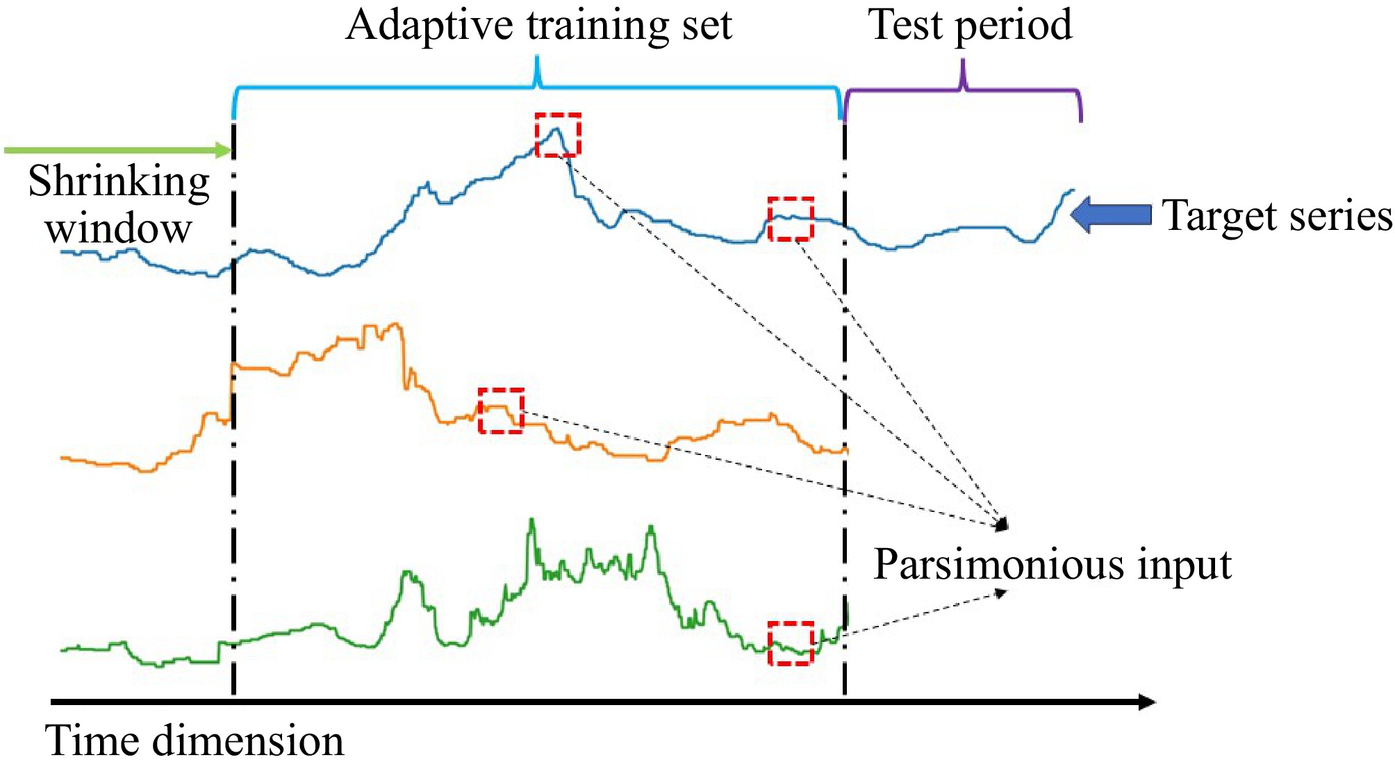
Figure 1. 

Partitioning scheme of SVRIMSE.

Step 2. One set of explanatory variables among a large set of variables is chosen. Although it is well-known that more explanatory variables can help the model learn more complex knowledge from the data, irrelevant variables will cause a burden on the model's learning and degrade the performance.

Step 3. One combination of time lags is chosen, which serves as the input for the learning candidate. Different from the existing works, various combinations of time lags are considered in our model. For example, a forecasting model with time lag three is usually trained by feeding data at t-1, t-2, and t-3, but our model can utilize combinations of the lags, such as t-1 and t-3.

Step 4. Then, the SVR models with different hyper-parameters using the corresponding combinations of time lags are trained based on the chosen shrinking window size.

Step 5. After training, the model is applied to the validation set, and the corresponding error metric is calculated.

Step 6. All errors on the validation sets are compared and the model with the minimum error is the final SVR.

Step 7. The final SVR is re-trained with the selected SVR's hyper-parameters, shrinking window size, a combination of explanatory variables, and time lags.

Step 8. Finally, the retrained SVR is applied to the test set.

The SVRIMSE effectively captures both temporal and cross-variable dependencies through its integrated components, particularly the Intelligent Model Search Engine. This component is pivotal in identifying critical variables and the appropriate time lags that optimize predictive performance, assessed rigorously on a validation dataset. In the process of model development, the Intelligent Model Search Engine first conducts a systematic search across potential predictors and their corresponding time lags. This search is not arbitrary; it is finely tuned to discern which variables and their historical values (time lags) most significantly influence the target variable, thereby elucidating cross-variable dependencies. The identified variables are those that consistently show a predictive relationship with the outcome across various scenarios within the validation set. Simultaneously, by determining the optimal time lags for these variables, the Intelligent Model Search Engine captures the temporal dependencies crucial for time-series forecasting. These time lags reflect how past values of one or more variables influence future values of the target variable, which is essential for understanding the dynamics within the data. Following this variable and lag selection phase, the SVR component of the model is trained. SVR is particularly well-suited for this task as it excels in modelling non-linear relationships. By training the SVR on the variables and time lags selected by the Intelligent Model Search Engine, the model not only learns the direct relationships but also the intricate non-linear interactions among the variables over time. This comprehensive approach ensures that SVRIMSE not only captures, but also leverages these dependencies to enhance forecasting accuracy.

Ship size

There are three types of tanker vessels in the data collected in this study. Table 1 summarizes the key features. Aframax ships refer to medium-sized crude oil tankers with a deadweight tonnage ranging between 80,000−120,000 metric tons. Tankers of this size have a cargo-carrying capacity between 70,000−100,000 metric tons, with an average cargo-carrying capacity of approximately 750,000 barrels. Due to their advantageous size, Aframax tankers are ideal for short to medium-haul oil trades and are primarily used in areas that do not have very large ports to accommodate bigger crude oil tankers or very large crude oil tankers. Vessels falling within this range are also referred to as the 'workhorses' of the world tanker fleet, as they carry a large number of oil products from many producing regions and can serve most of the ports in the world.

Suezmax ships are the largest marine vessels that can meet the restrictions of Suez, and transit the Suez Canal in a laden condition. Suezmax ships have a deadweight tonnage ranging between 120,000−200,000 metric tons. Ships from this size category are larger than the Aframax ships, and they can carry about 800,000 to more than 1,000,000 barrels of crude oil. After the expansion of the Suez Canal from 18 to 20.1 m in 2009, it is possible for a Suezmax ship up to 200,000 deadweight tonnage to pass through it.

Very Large Crude Carriers (VLCC) have a size ranging between 180,000-320,000 deadweight tonnage and they are capable of passing through the Suez Canal in Egypt. As a result, VLCC vessels are largely deployed around the North Sea, Mediterranean, and West Africa. Compared to the other smaller crude oil tankers, VLCCs are the larger vessels that provide better economies of scale for crude oil shipment. Specifically, VLCC ships are capable of carrying between 1.9 million and 2.2 million barrels of crude oil, and offer good flexibility for operating in ports with some depth limitations.

Data description and pre-processing

The data investigated in this study come from various databases including Bloomberg Inc., Lloyd's List Maritime Intelligence, Tradewinds, and Clarkson Shipping Intelligence. A suitable and correct data pre-processing approach helps the machine learning model generate accurate outputs. First, the first differences of all time series are calculated to remove the linear trend. Computing the first difference of time series is a common approach in the forecasting literature. After obtaining all the first differences, the first differences are normalized for the implementation of machine learning models. The max-min normalization is implemented in this study. We assume that the maximum and minimum of the training set are x_max and x_min, respectively. The data are scaled into the range [0,1] using the following Eq (8):

where, x_normalized and x represent the normalized and original time series, respectively.

Each model has several hyper-parameters that define the specific structure and affect the performance dramatically. To determine the suitable hyper-parameters for each model, the last-block cross-validation is adopted^[39]. The time series are split into training, validation, and test sets. The data from 2016 and 2017 are validation and test set, respectively. The hyper-parameters that achieve the minimum error on the validation set are selected as the winner.

Comparative analysis of all models

The analysis of the comparative results consists of two perspectives. First, the accuracy demonstrates the success of the proposed model in forecasting time charter rates. Second, the selected explanatory variables indicate their significant contribution to accurate forecasts of time charter rates. Three forecasting error metrics are utilized to evaluate the accuracy of these models. The first error metric is the classical Root Mean Square Error (RMSE) whose definition is:

where, L is the size of the test set, x_j and $ \hat{{x}_{j}} $ are the raw data and predictions. Another error metric implemented in the paper is the Mean Absolute Scaled Error (MASE)^[40]. The definition of MASE is given in Eq (10):

where, T represents the size of the training set. The denominator of MASE is the mean absolute error of the in-sample naive forecast. The third error metric is the Mean Absolute Percentage Error (MAPE) whose definition is described by Eq (11):

The comparative results of these three time charter rates in terms of RMSE, MAPE, and MASE are presented in Tables 2−4. According to the comparative results, we can claim that the proposed SVRIMSE outperforms the other models in terms of RMSE, MAPE, and MASE. The SVRIMSE achieves better performance than the SVR, which emphasizes the significance of training set size optimization and feature selection. The RIMSE also achieves great success in time charter rate forecasting because its structure is determined under the same framework as SVRIMSE. However, the learning candidate of RIMSE is linear, it cannot learn the complex non-linear patterns as SVRIMSE does. The models with the input of all variables cannot outperform the Naïve forecast, because the redundant variables hinder the learning of valuable relationships. The ridge regression performs much worse and its MASE is the lowest on all datasets because of its linear structure and lack of input optimization. As a result, we claim that the SVRIMSE can learn the knowledge of the freight market efficiently. The comparison of forecasts on the test set is visualized in Figs 2−4. All models predict the trend of Aframax time charter rates accurately according to Fig. 2. According to Fig. 3, there is a huge deviation from ridge regression's forecasts and raw data. The SVRIMSE forecasts the trend and values of these three-time charter rates accurately.

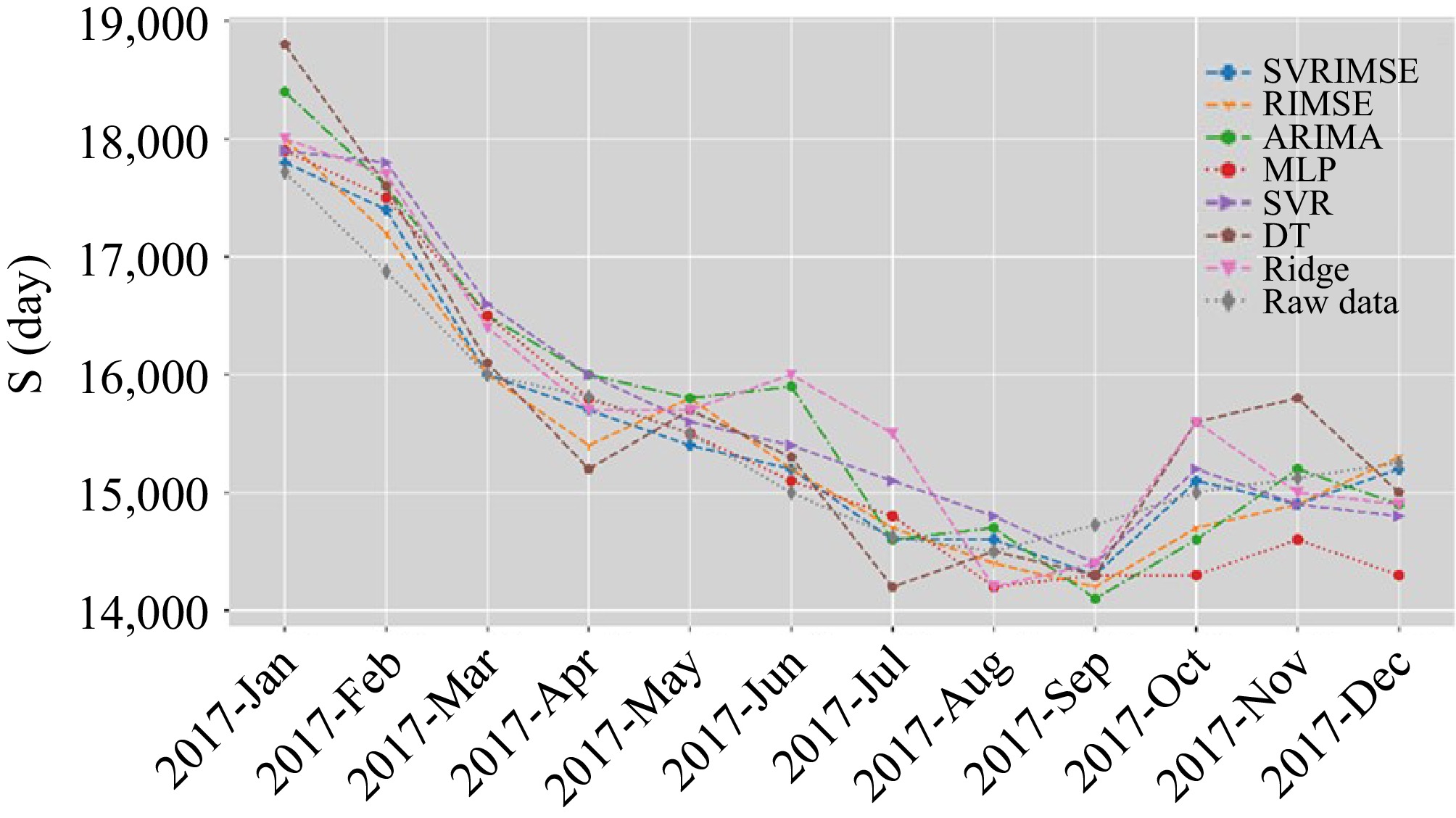
Figure 2. 

Comparison of forecasts on Aframax time charter rates.

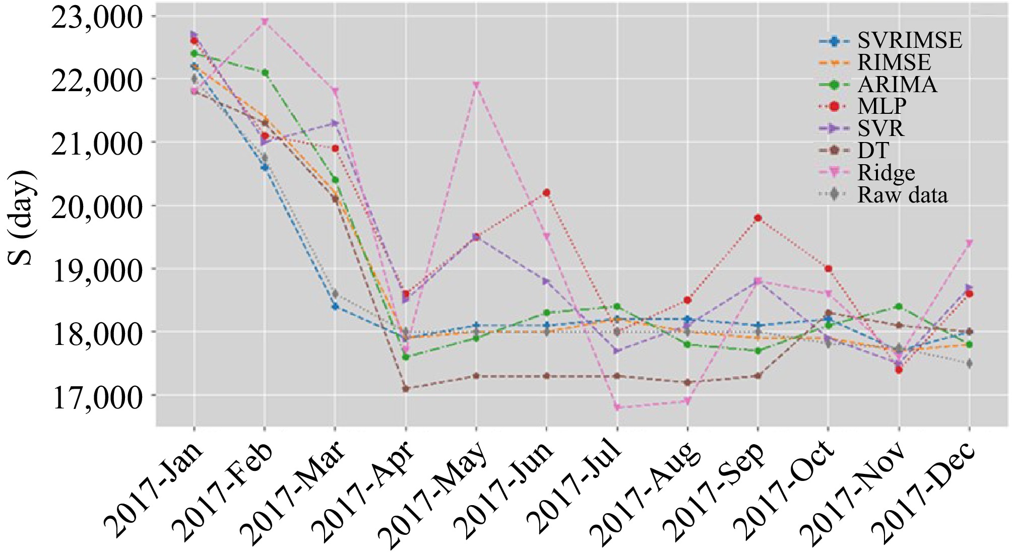
Figure 3. 

Comparison of forecasts on Suezmax time charter rates.

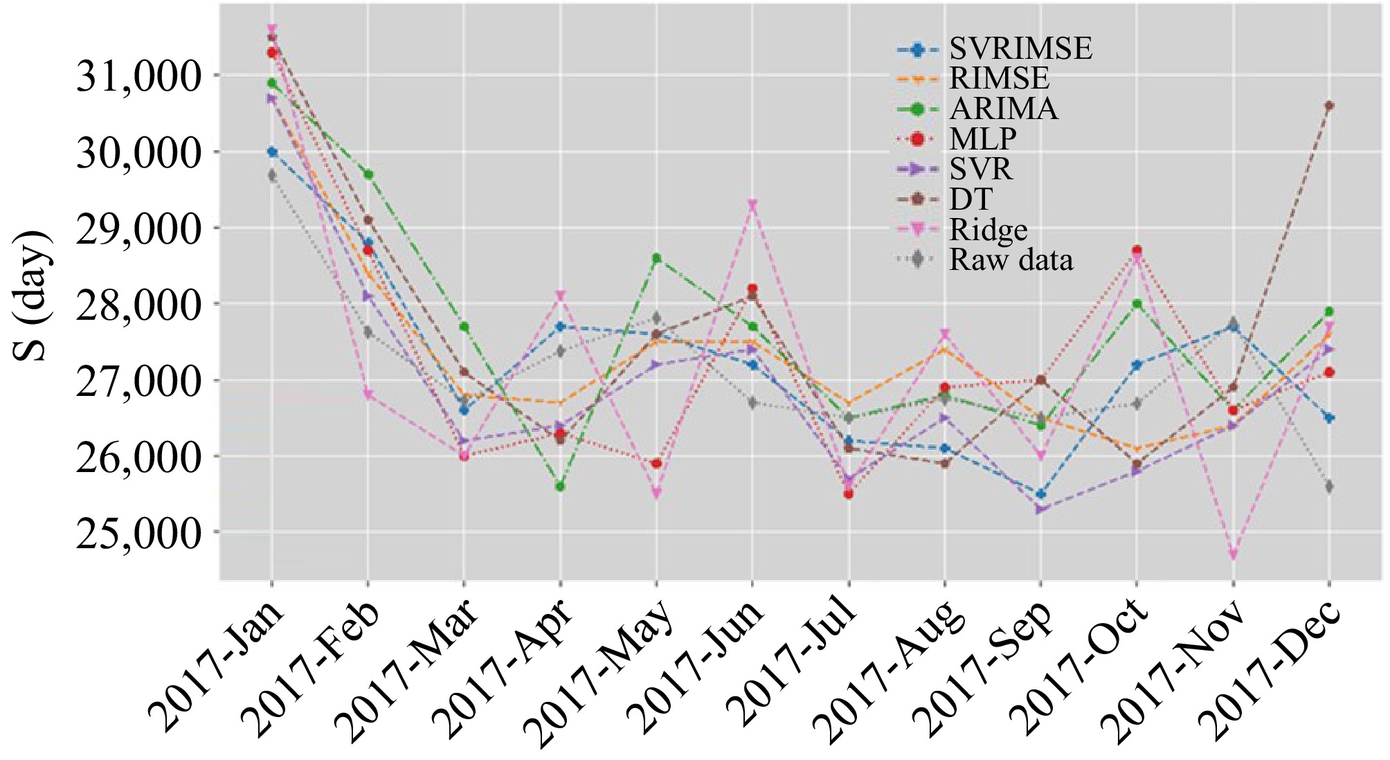
Figure 4. 

Comparison of forecasts on VLCC time charter rates.

The selected variables for forecasting time charter rates are summarized in Table 5. The selection of the corresponding variable indicates their significant contribution to forecasting time charter rates. The Fleet Development (Number) and Scrap Value are selected for these three-time charter rates, which demonstrates their contribution to forecasting time charter rates most. Newbuilding prices are used for Aframax and Suezmax, which indicates the newbuilding prices contribute less than the Fleet Development (Number) and Scrap Value. In addition, the Fleet Development (Million DWT), Orderbook (DWT), and Orderbook (Number) are used once because of their general influence on the time charter rates.

According to comparative results, the SVRIMSE outperforms the other models, which demonstrates its success in forecasting time charter rates. The SVRIMSE achieves better performance than RIMSE because the SVR can mine non-linear and complex relationships among various variables. The primary factor that contributes to the superior performance of SVRIMSE over RIMSE is its ability to capture and leverage non-linear information inherent in complex datasets. Specifically, RIMSE is constrained by its reliance on the Ridge regression model, which, although robust in handling multicollinearity, is fundamentally limited to linear interactions. This linear approach restricts RIMSE from effectively modelling the intricate and dynamic non-linear patterns that are prevalent in volatile markets such as shipping. In contrast, SVRIMSE incorporates SVR, which is inherently designed to handle non-linear relationships. SVR achieves this through the use of kernel functions, which transform the data into a higher-dimensional space where non-linear relationships can be linearized and thus more effectively modelled. This capability allows SVRIMSE to adapt to the complex and non-linear dynamics that characterize the shipping market's multivariate time series data. Moreover, the shipping market's volatility introduces rapid changes in trends and anomalies, which are better captured by the non-linear modelling approach of SVR. The SVR's framework, equipped with features like regularization and kernel-based learning, is more adept at managing unpredictability and ensuring robustness against overfitting compared to the linear methods used in RIMSE. The combination of SVR's advanced non-linear modelling capabilities and the iterative feature selection process of RIMSE within SVRIMSE further enhances its performance. By selectively incorporating significant variables and their respective time lags that best capture the temporal and cross-variable dependencies, SVRIMSE not only maintains model simplicity and computational efficiency, but also significantly improves forecasting accuracy. The other machine learning models fail to forecast the time charter rates accurately, because of the redundant explanatory variables. Although machine learning algorithms are good at extracting complex patterns based on more variables, the redundant variables convey much noise and degrade the performance. The success of the SVRIMSE demonstrates the importance of the objective design of the model and the information within the explanatory variables is non-linear.

This paper proposes a new framework for establishing the SVRIMSE to forecast the time charter rates of three categories of tankers, the Aframax, Suezmax, and VLCC. The forecasting process optimizes the SVR's hyper-parameter, training set size, memory size, and input variables. A comprehensive comparison of the SVRIMSE and other forecasting models is conducted, and three forecasting error metrics are computed to evaluate the performance. In addition, the SVRIMSE outperforms the RIMSE, which confirms that there are complex and non-linear relationships among these explanatory variables and time charter rates. The SVRIMSE selects more variables compared with the RIMSE because the linear structure of RIMSE cannot extract complex information from those variables. This paper also reveals the explanatory variables which contribute to the accurate forecasts of time charter rates significantly. The Fleet Development (Number) and Scrap Value are the most significant explanatory variables because they are selected to forecast time charter rates of all ship sizes. The Fleet Development (Number) indicates the current number of ships in operation all over the world and influences the time charter rates significantly based on domain knowledge. Scrap values also have the potential to affect charter rates by indicating the possibility of the deconstruction of ships. When the scrap values are high, the shipowners may prefer to dismantle the older ships instead of managing them.

The proposed forecasting framework provides practical implications for decision-making in the maritime industry. From the industry players' perspective (e.g., shipowners, charterers, and operators), the proposed framework offers a reliable tool for forecasting time charter rates, enabling better planning, and optimization of fleet deployment. By identifying key explanatory variables that influence charter rates, stakeholders can make informed decisions regarding vessel allocation, contract negotiations, and risk management. For example, shipowners can use the model to determine optimal charter durations or adjust their strategies in response to market fluctuations, while charterers can leverage the forecasts to secure cost-effective contracts. From the related investors' perspective, the model provides valuable insights into the dynamics of the freight market, aiding in the assessment of investment opportunities and risks. Investors can use the forecasts to evaluate the profitability of investing in specific vessel types or market segments, as well as to anticipate market trends and adjust their portfolios accordingly. Additionally, the model's ability to objectively identify significant variables can help investors understand the underlying drivers of charter rate volatility, enhancing their ability to make data-driven investment decisions. By bridging the gap between theoretical forecasting and practical decision-making, our framework not only advances the academic understanding of freight market dynamics, but also provides actionable insights for industry stakeholders and investors, ultimately contributing to more efficient and informed operations in the maritime industry.

The limitation of this study includes the application of ship types and data availability. The proposed framework was tested exclusively on three types of tankers. Its applicability to other vessel types, for instance, bulk carriers, remains unverified. Additionally, the exclusion of variables such as regulations and fuel price volatility may restrict the model's ability to capture emerging market dynamics. If more data is available, the proposed forecasting model could be further verified regarding accuracy.