Full-space magnetic coupling wireless power transfer system and magnetic energy control method

Magnetic coupling wireless power transfer (MC-WPT) technology enables the contactless transmission of electrical energy from a source to a load based on the principle of magnetic field coupling^[1−3]. This technology provides an effective solution for supplying power flexibly to mobile devices without interruption and for ensuring the safe and reliable operation of electrical equipment in harsh, unattended environments, such as deep-sea, deep-space, and underground applications. Consequently, it has become a prominent research topic in the fields of electrical engineering and automation. Currently, this technology has been successfully applied in various sectors, including electric vehicles^[4], consumer electronics^[5], and home appliances^[6,7].

At present, efficient energy transfer in MC-WPT systems can only be achieved within a limited spatial region. To enhance its spatial degrees of freedom, existing research has primarily focused on designs involving three-dimensional magnetic coupling structures^[8], coil arrays^[9], and multi-transmitter coil configurations^[10]. These methods improve the power transfer capability of the system by extending the spatial coverage of the magnetic field, but they still suffer from the following limitations: (1) The expansion of the magnetic energy distribution range leads to excessively high magnetic field intensity in non-target areas, aggravating electromagnetic interference and environmental safety concerns; (2) Limited by the inherent property that magnetic field lines cannot intersect, 'ineffective power transfer zones' inevitably exist near the coupling structures. Within these zones, effective energy transfer cannot be achieved due to the absence of magnetic field lines orthogonally penetrating the receiver coil, making it challenging to realize a truly full-space and omnidirectional wireless power supply.

To eliminate 'ineffective power transfer zones' and suppress electromagnetic leakage in non-target areas, the magnetic energy directional tracking control method has attracted wide attention. This method dynamically adjusts the magnetic field distribution and directs it toward the target position^[11−16]. To enhance the spatial adaptability of the MC-WPT system, current research mainly focuses on two types of control methods. The frequency-modulation-based magnetic energy regulation strategy maintains high output power and transmission efficiency by dynamically adjusting the system operating frequency^[11−13]. The phase-control-based energy beamforming technique achieves directional magnetic field shaping by regulating the current phase of each excitation coil. This effectively suppresses magnetic leakage and improves the system's efficiency^[14−16]. However, according to the Biot-Savart law, the direction of the magnetic field vector at any point in space is uniquely determined under a fixed coil configuration. Existing frequency modulation and phase modulation methods can only adjust the magnitude of the magnetic field vector in this direction, without altering its orientation. Furthermore, frequency modulation is prone to frequency splitting, which introduces disturbances to system stability, while phase modulation imposes stringent requirements on inverter output quality and involves higher control complexity. Therefore, how to achieve active control of the magnetic field direction, thereby dynamically constructing effective power transfer paths in three-dimensional space, has become a key challenge for realizing truly full-space wireless power transmission.

Accordingly, this paper proposes a multi-node three-dimensional (3D) orthogonal power transfer architecture that comprehensively considers both transmission range and freedom of movement. This architecture uses a 3D orthogonal coil structure as its fundamental node and includes both centralized and distributed power transfer modes. It allows for the on-demand selection of orthogonal coils, effectively enhancing the power transfer range. Building upon this, a cooperative control criterion for multiple excitations is established. By comprehensively controlling the coil combination structure and the corresponding current amplitudes, the magnetic field strength and direction at any point within a given space can be precisely controlled. This eliminates the influence of 'ineffective power transfer zones' and achieves omnidirectional, full-angle, low-leakage, precise, and efficient power transfer over a large area.

Based on a three-coil concentric orthogonal structure as nodes, this paper constructs a multi-node wireless power transfer network. A schematic diagram of the proposed power transfer architecture is shown in Fig. 1.

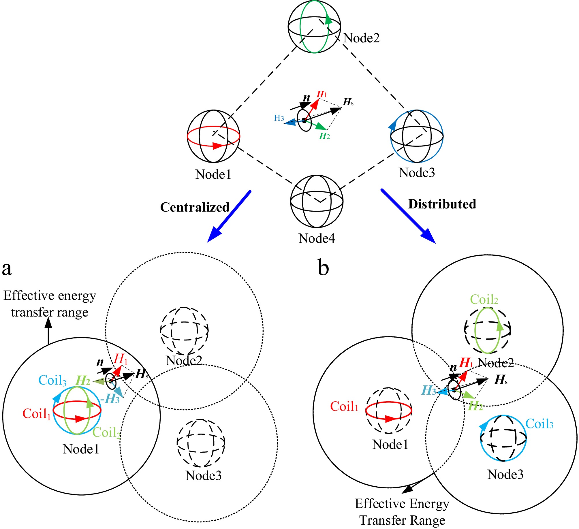
Figure 1. 

Multi-node wireless power transfer network architecture. (a) Centralized 3D orthogonal power transfer mode. (b) Distributed 3D orthogonal power transfer mode.

Based on the configuration of 3D orthogonal transmitting coils, the system supports two operation modes: centralized and distributed 3D orthogonal power transfer. In the centralized power transfer mode, the three orthogonal coils are concentrated at a single physical node. In the distributed power transfer mode, three orthogonal coils are placed at three independent nodes, with one orthogonal coil located at each node, as shown in Fig. 1a and b. In the schematic, solid black circles represent the effective power transfer range; within the 3D coil diagrams, solid lines indicate excited coils, while dashed lines represent unexcited coils.

Both of the aforementioned power transfer modes are capable of controlling the magnetic field orientation at an arbitrary point in space. However, due to the inherent spatial decay of magnetic fields, a single node can only transfer energy effectively within a limited distance, which defines the effective power transfer range. Furthermore, the required current amplitudes in the individual coils to generate an identical magnetic field vector vary across different spatial regions and between the different transfer modes. Consequently, this leads to variations in coil losses and overall system efficiency. Therefore, the optimal power transfer mode can be selected based on the specific spatial region.

The synthesized magnetic field vector at the position of the receiving coil is analyzed. The vector relationship shown in Fig. 1 can be expressed by Eq. (1) as:

where, H_i is the magnetic field vector generated by Coil i, i is the index of the selected coil, H_s is the resultant magnetic field vector synthesized by the three orthogonal coils, and n is the normal vector of the receiving coil plane. H_s//n indicates that the synthesized magnetic field vector from the three orthogonal coils is parallel to the normal vector of the receiving coil. Note that boldface letters denote vectors, while non-boldface letters denote scalars throughout this paper.

Based on Fig. 1a, b and Eq. (1), it can be concluded that when the receiving coil is positioned within the local power transfer space and its size is significantly smaller than that of the transmitting coil, it can be approximated as a point mass within the local power transfer network. By selecting the three orthogonal coils at Node 1, Node 2, and Node 3 as transmitting coils, a multi-excitation cooperative control scheme is established. This scheme directs the synthesized magnetic field at the location of the receiving coil toward the direction of the coil's normal vector, thereby achieving magnetic energy steering in the desired direction.

Field spatial distribution modeling

A magnetic field distribution model is established for the proposed multi-node power transfer architecture. A Cartesian coordinate system is defined with the geometric center of Coil 1 as its origin. A schematic of the overall setup is shown in Fig. 2, where the coordinates of the field point P are (x₀, y₀, z₀), and the center of each coil, Oᵢ, is located at (Xᵢ, Yᵢ, Zᵢ) for i = 1, 2, 3.

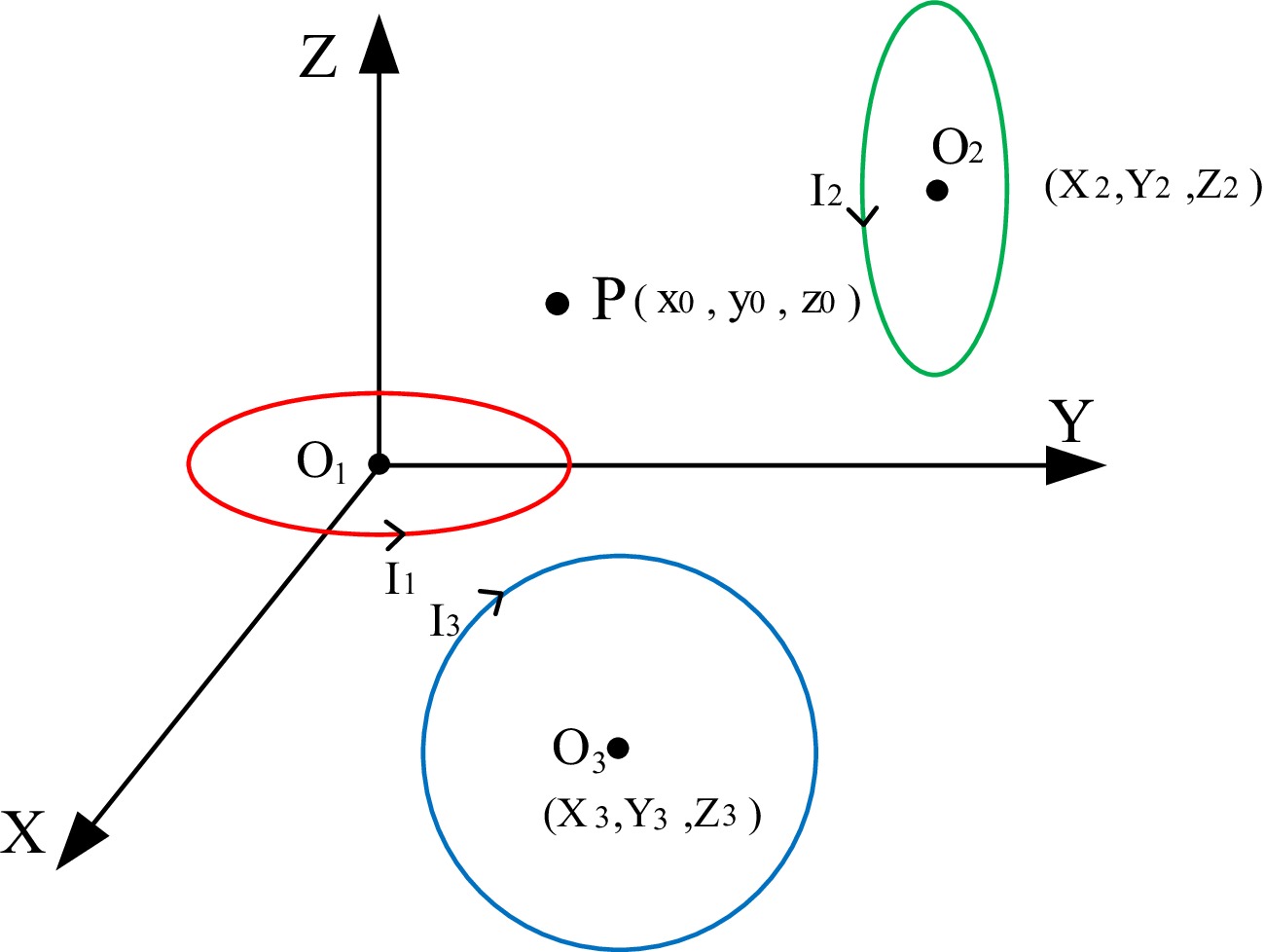
Figure 2. 

Schematic diagram of the three orthogonal coils and the receiving center point.

Since the MC-WPT system operates in a time-varying field environment, the analysis incorporates Maxwell's equations for time-varying fields and introduces the magnetic vector potential A, which satisfies the following expression:

Substituting Eq. (2) into Maxwell's equations and combining it with the Biot-Savart law, the integral form of the spatial magnetic field generated by excitation Coil 1 at field point P is derived as:

where, I₁ is the excitation current of Coil 1, r is the distance from the field point to the center of Coil1, r₁ is the radius of Coil 1, and k_m is the electromagnetic wavenumber.

where, (x_i,y_i,z_i) represents the coordinates of the center point P in the coordinate system of Coil i (i = 1, 2, 3); R₂ and R₃ are the rotation matrices from Coil 1 to Coil 2 and 3, respectively; and θ₂, θ₃ denote the clockwise rotation angles from Coil 1 to Coils 2 and Coils 3.

Since the effective operating range of the MC-WPT system lies within the inductive near-field region, where the product of the electromagnetic wavenumber and the propagation distance is much less than 1, the magnetic field components in the Cartesian coordinate system are derived by incorporating the preceding analysis and substituting Eq. (4) into Eq. (3), yielding:

where, a_r is the coil radius, x_i, y_i, z_i are the unit vectors along the fundamental directions of the local coordinate system for Coil i at the center point P, r_i is the distance between the center point P and the center of Coil i, and H_ii is the magnetic field vector generated by Coil i in its own coordinate system.

By applying the inverse coordinate system rotation and incorporating Eq. (5), the expression for the spatial magnetic field excited by Coil i at the center point P, described in the O₁ coordinate system, is generalized as:

where, H_il denotes the magnetic field vector of Coil i represented in the O₁ coordinate system.

By applying the superposition theorem, the x, y, and z components of the total resultant magnetic field generated by the three orthogonal coils can be expressed as:

where, H_x, H_y, and H_z are the X,Y, and Z components of the resultant magnetic field, respectively, and H_ui1 represents the magnetic field vector component of Coil i along the u-axis in the O₁ coordinate system, with u = x, y, z.

The resultant magnetic field of the three orthogonal coils is given by:

where, H_s denotes the magnitude of the total magnetic field at point P generated by the three orthogonal coils. The receiving coil's normal vector n is then converted to the basis vectors by incorporating the plane normal from Fig. 1 into Eq. (8):

where, a, b, and c are the coefficients of the unit vectors, respectively.

Substituting Eqs (8) and (9) into the right-hand side of Eq. (1) yields the proportional relationship of the corresponding magnetic vector components.

where, k is a proportional coefficient.

From the law of electromagnetic induction, the magnetic flux density magnitude is a function of the current magnitude, as expressed by:

where, T_i is the geometric coefficient in the magnetic field equation for orthogonal coil i, and I_i is the excitation current of the same coil.

Substituting Eq. (11) into the right-hand side of Eq. (8) and simplifying yields:

where, e_ri is the unit vector pointing from the current element on orthogonal coil i toward the center point P.

Expressing Eq. (12) in the frequency domain using the instantaneous current values yields:

where, I_i, ω_i, and φ_i are the amplitude, angular frequency, and phase of the excitation current I_i, respectively.

A qualitative analysis of Eq. (13) reveals that when the currents of the three excitation coils have the same frequency and are in phase, the direction of the resultant magnetic field is determined solely by the ratio of their amplitudes and remains constant over time, as shown in Eq. (14).

Based on this, the magnetic vector control criterion proposed in this paper operates as follows: under the condition that the excitation currents flowing through the transmitter coil array of the MC-WPT system share the same frequency and phase, the direction of the resultant magnetic vector can be controlled solely by adjusting the ratio of the three current amplitudes applied to the selected orthogonal coils. Furthermore, provided that this amplitude ratio is maintained, the magnitude of the resultant magnetic vector can be controlled by adjusting the absolute values of the three excitation currents without affecting its direction. This, in turn, enables dynamic 3D magnetic vector control for the distributed wireless power transfer system.

Given a desired magnetic field direction at point P in three-dimensional space, combining and transforming Eqs (7) and (10) yields a matrix equation relating the electrical parameters, geometric parameters, and desired vector direction ratios of the MC-WPT system:

where, T_ui denotes the current coefficient of the orthogonal coil i for the magnetic field component along the u-axis, with u = x, y, z.

By solving the matrix equation Eq. (15), the solution for the current amplitude ratio of the three orthogonal coils can be obtained as:

Given the desired magnetic field at the center point, and by combining Eqs (14) and (16), the solving function can be defined as:

From Eq. (17), it can be seen that by applying the specified excitation currents to the three orthogonal coils, a magnetic field vector with the desired magnitude and a direction perpendicular to the coil plane is generated at the center point.

For the proposed system power transfer architecture in this paper, the variation in the central coordinates of the coil nodes influences the current magnitudes within the excitation current set derived from the magnetic vector control criterion. This, in turn, leads to differences in the coil loss of the MC-WPT system during operation. Consequently, the system optimization objective is defined as the magnetic coupling mechanism loss, which is primarily dependent on the excitation current amplitude and thus correlated with the node coordinates. That is:

When multiple sets of current combinations satisfy the desired magnetic field direction and magnitude for a distributed power transfer system, each set of three current amplitudes is substituted into Eq. (18). This yields the corresponding magnetic coupling coils loss for each set, and then the set with the minimum loss is selected. This provides the optimal three-orthogonal-coil node combination within the proposed single-node and multi-node system architectures.

Control method for excitation current

According to Eq. (14), the desired magnetic field magnitude and direction can be obtained by modulating only the amplitude of the excitation currents in the three orthogonal coils. The proposed current control method is illustrated in Fig. 3. L_i, C_i, and R_i represent the transmitter coil's self-inductance, series compensation capacitance, and equivalent series resistance, respectively. L_fi and C_fi denote the parallel inductor and capacitor in the chopper circuit. VD_i and S_i refer to the freewheeling diode and switching transistor in the chopper circuit, while S_ii indicates the switching transistor in the inverter circuit. U_ni represents the output voltage of the chopper circuit, u_i and i_i correspond to the output voltage and current of the inverter, V_D is the DC input voltage, and α_i denotes the duty cycle of the chopper circuit.

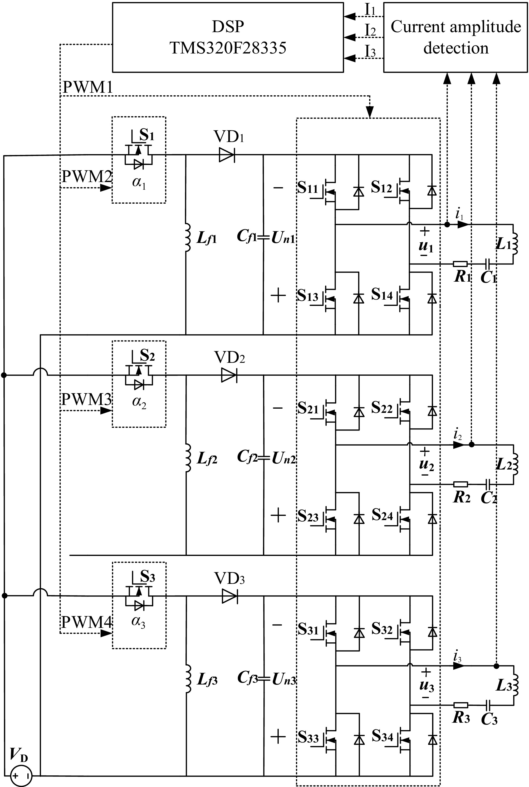
Figure 3. 

Excitation current control circuit diagram.

As shown in Fig. 3, the chopper circuit adjusts the DC voltage from the source V_D to generate the output voltage U_ni. Based on the operating principle of the Buck-Boost circuit, the following relationship holds:

Here, α_i is the duty cycle of the control signal for the switching transistor S_i in the chopper circuit. It can be seen that when α_i < 50%, the circuit acts as a buck converter, and when α_i > 50%, it acts as a boost converter.

The regulated DC voltage U_ni is then inverted by the inverter into a square wave. Based on the fundamental harmonic approximation, this can be considered equivalent to a sinusoidal wave ui of the same frequency, with an amplitude U_i given by 4 U_ni/π.

Since the three orthogonal coils are mutually decoupled, the mutual inductance between them is not considered. Furthermore, as the three coils have identical structures, we can let L₁ = L₂ = L₃ = L, C₁ = C₂ = C₃ = C, R₁ = R₂ = R₃ = R.

To ensure the system operates at resonance, the following condition must be satisfied:

In Eq. (20), ω = 2πf, where f is the operating frequency of the system. The amplitude of the output current i_i, denoted as I_i, can then be expressed as:

From Eq. (21), it can be seen that with the DC voltage source V_D and the equivalent coil resistance R being fixed, the excitation current amplitude I_i is dependent only on the duty cycle α_i of the Buck-boost chopper circuit.

By combining Eq. (21) and Eq. (17), the solution function for the duty cycle α_i can be obtained as follows:

The verification of the centralized magnetic energy regulation principle is divided into two parts: the verification of the magnetic vector direction and magnitude for the centralized power transfer system. A 3D model of the centralized orthogonal coil power transfer structure, established in the COMSOL finite element simulation software, is shown in Fig. 4a. The simulation parameters are listed in Table 1.

To verify the correctness of magnetic field direction control, the desired magnetic field direction is set to the X, Y, and Z directions, respectively. A point at the center of the cubic air domain surrounding the centralized power transfer architecture is selected as the verification point. This point is used to verify the different desired directions, and a schematic of the verification is shown in Fig. 4b.

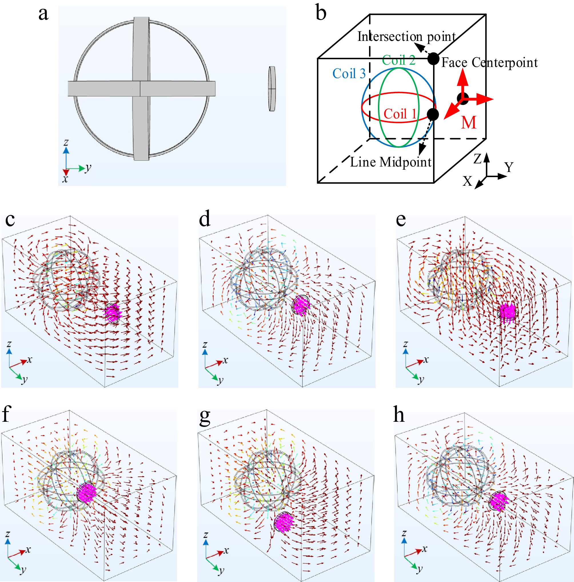
Figure 4. 

(a) Centralized energy transfer architecture model. (b) Schematic diagram of magnetic vector direction verification setup for centralized power transfer. (c)−(e) Magnetic vector different direction simulation diagram of centralized architecture. (f)−(h) Simulation diagram of the magnetic vector at different points in the centralized architecture.

Based on the coil parameters designed in Table 1 and in conjunction with Eq. (5), a suitable magnetic field magnitude of 7 A/m is determined through rational planning. All subsequent verification and implementation in this paper are based on this value. Then, according to Eq. (17), the required excitation current magnitudes are calculated for when the receiving coil's normal direction is aligned with different desired magnetic field directions. The current parameter settings for the magnetic field direction control verification are listed in Table 2.

The parameters given in Table 2 are input into the 3D centralized orthogonal coil simulation model established in COMSOL. With the operating frequency set to 91 kHz, the simulation is performed, yielding the volume arrow plots of the magnetic field intensity on the receiving coil plane for different orientations, as shown in Fig. 4c-e. The corresponding magnetic field magnitudes are listed in Table 3.

As can be seen from Fig. 4c-e and Table 3, when the normal direction of the receiving coil plane is oriented towards the X, Y, and Z directions, respectively, and the excitation currents for the three orthogonal coils of the centralized power transfer architecture are applied, the magnetic vector arrows on the receiving coil are maximized in the positive X, positive Y, and positive Z directions, respectively. This indicates that the magnetic field direction is consistent with the desired direction, and also demonstrates that the magnetic field regulation criterion proposed in this paper can generate a magnetic field that aligns with the intended direction.

To validate that the magnetic field magnitude of the centralized power transfer system is controllable, it is necessary to select multiple target field points. Based on the desired magnetic field vector magnitude to be generated at each point, algorithm computations are performed to derive the corresponding current amplitude ratios, as well as the specific current amplitude parameters for the three orthogonal coils under the given magnetic field strength. An intersection point on a line, a midpoint of a line, and a midpoint of a surface within the same air domain are selected as the field points for verification, as illustrated in Fig. 4b. The field point locations, desired magnetic field directions, desired magnetic field magnitudes, and excitation current parameters are listed in Table 4.

The given current amplitude parameters are input into the COMSOL-based simulation model of the centralized three-dimensional orthogonal coils. The simulation results yield the magnetic field intensity vector arrows on the receiving coil plane at different field point positions, as shown in Fig. 4f-h, and the corresponding magnetic field magnitudes are listed in Table 5.

As observed from Fig. 4f-h and Table 5, the magnetic field magnitude at different field point locations can be regulated to the desired steady-state value. The magnetic field control method enables the generation of corresponding current excitation combinations to achieve precise control of the magnetic field strength at various positions, including line intersections, line midpoints, and surface midpoints.

Simulation of distributed magnetic control

The simulation of the distributed magnetic energy steering criterion is performed to validate both the direction and magnitude of the magnetic field generated by the distributed system at a common field point. Given the existence of multiple excitation combinations, it is necessary to determine the optimal node configuration and the corresponding current amplitude parameters.

The distributed system is constructed using three nodes, with their centers positioned at the vertices of an equilateral triangle. The three orthogonal coils at each individual node are coplanar. A schematic diagram of this configuration is shown in Fig. 5a.

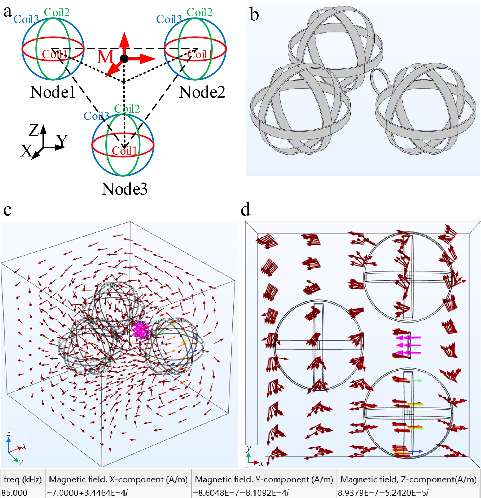
Figure 5. 

(a) Spatial diagram of distributed power transfer architecture. (b) Distributed simulation model. (c) Magnetic vector simulation of distributed architecture with expected magnetic field direction in the X direction.(d)Top view of Fig. 5c.

The parameters of the COMSOL simulation model are listed in Table 6, and a schematic of the simulation model is shown in Fig. 5b.

The central point M of the distributed power transfer system is selected as the verification point. To comprehensively validate the magnetic vector control criterion in terms of both magnetic field direction and magnitude, it is necessary to perform verification with the X, Y, and Z directions, each serving as the desired magnetic field orientation, and also to use 7 A/m as the desired magnetic field magnitude for validation. Synthetically, this requires setting the red arrows in Fig. 5b as the desired directions to conduct the corresponding validation of magnetic field direction and magnitude. This section takes the X-direction as an example. After specifying the field point location, the desired magnetic vector direction, and magnitude, multiple sets of current amplitude parameters are derived through the magnetic field steering method. These sets are then evaluated using the optimal combination selection formula for the distributed power transfer system to determine the optimal node configuration and the corresponding current amplitude parameters. Subsequently, the currents in the coils of the selected different nodes are set to the respective amplitudes according to the algorithmic results. The magnetic field direction is then visualized via streamlines, and the components of the magnetic vector at point M are obtained to complete the verification.

Following the aforementioned procedure, parameters are configured for the simulation model established in Fig. 5b. The current combination parameters corresponding to the desired X-direction are presented in Table 7, where Q1, Q2, and Q3 denote Node 1, Node 2, and Node 3, respectively.

Different excitation current combinations lead to varying coil losses. By substituting the current amplitudes of the different combinations from Table 7 into Eq. (18), the total current energy required for each combination can be derived. The corresponding results are shown in Fig. 6.

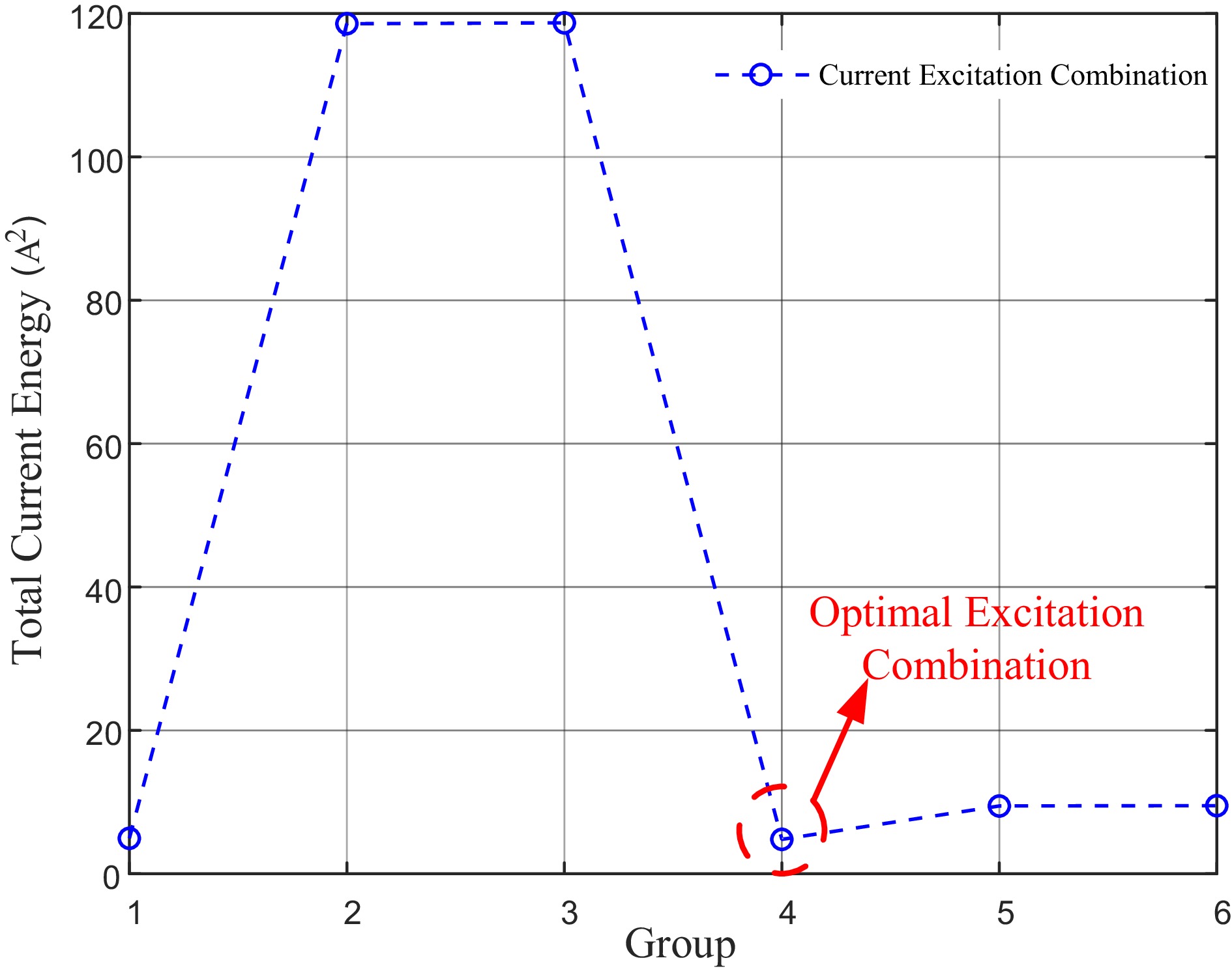
Figure 6. 

Line graph of total current power of different current excitation combinations with expected magnetic field direction in the X direction.

The current amplitude parameters of the aforementioned optimal combination are applied to the simulation model in Fig. 5b, with the operating frequency set to 91 kHz. The corresponding simulation results are presented in Fig. 5c-d.

As observed from Fig. 5c-d, the magnetic vector arrows on the receiving coil predominantly align with the positive X-direction, clearly indicating orientation along the predefined desired magnetic field direction. Furthermore, the magnetic field magnitude in the X-direction is 7.0139 A/m, which is in close agreement with the desired value.

To validate the feasibility and effectiveness of the proposed full-space magnetic energy steering method in this paper, an experimental setup is constructed as shown in Fig. 7.

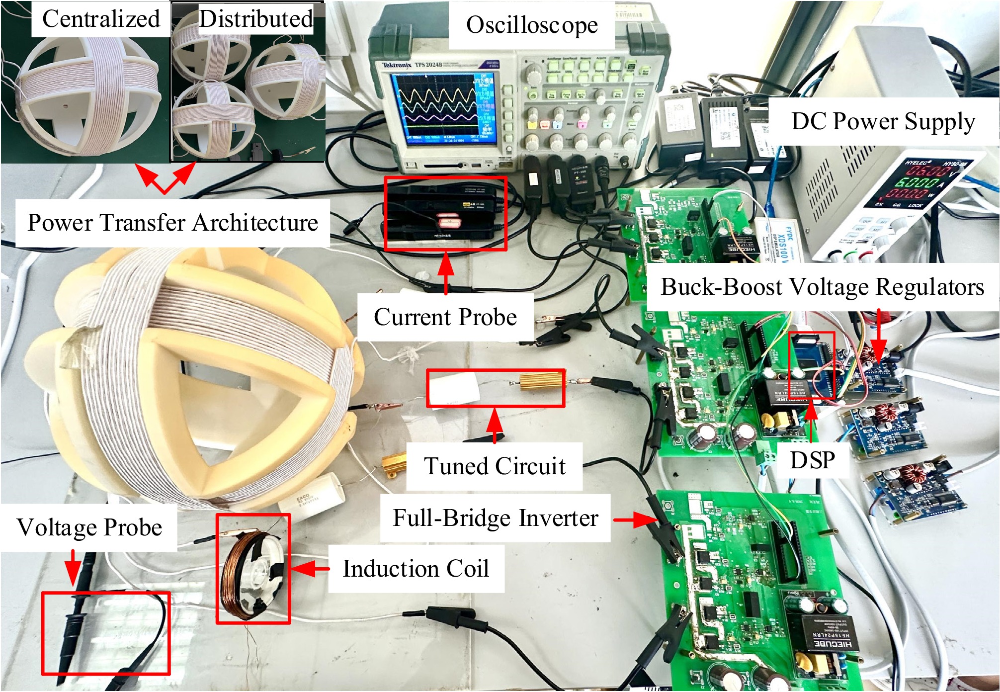
Figure 7. 

Schematic diagram of the experimental device for a centralized power transfer system.

The setup primarily consists of a DC power supply, three Buck-Boost voltage regulators, three full-bridge inverters, three Series-Series (SS) compensation networks, a power transfer architecture, and an inductive coil. On the receiver side, a compact one-dimensional magnetic field probe was designed and fabricated by winding multiple turns of enameled wire. This probe serves as a receiving coil to detect both the magnitude and direction of the synthesized magnetic field. The relationship between the induced electromotive force and the magnetic field strength is given by Eq. (23).

where, E is the electromotive force induced in the magnetic field probe coil by the alternating magnetic field, S is the cross-sectional area of the probe coil, N is the number of turns of the probe coil, and μ₀ = 4π × 10⁻⁷ N/A² is the permeability of free space. The circuit parameters of the experimental system are listed in Table 8.

Experimental verification of centralized magnetic energy control principles

To validate the correctness of the magnetic energy steering criterion, experimental verification is conducted on both the direction and magnitude of the spatial magnetic field vector. Since the verification methodology is identical, only the case with the desired magnetic vector direction along the X-axis is examined here.

First, the directional control of the magnetic field is verified. The excitation current parameters for the X-direction from Table 2, along with other relevant parameters, are applied to the experimental platform shown in Fig. 7. The X, Y, and Z components of the magnetic vector at field point M are detected using the magnetic field probe coil. The resulting transmitter coil currents and the induced voltage waveforms on the probe coil are shown in Fig. 8. Specifically, Fig. 8a-c presents the oscilloscope results for the X, Y, and Z components of the magnetic field, respectively.

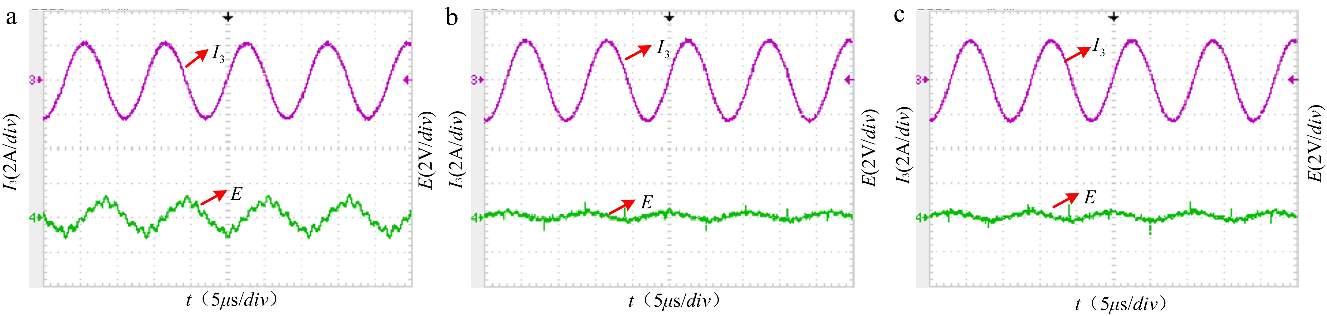
Figure 8. 

Experimental waveforms of X, Y, and Z components at point M with the expected magnetic field direction in the X direction.

As shown in Fig. 8, the X-component of the magnetic field at point M is dominant, while the Y- and Z-components are negligible. This indicates that the actual magnetic field direction aligns with the desired X-direction, demonstrating the capability of the proposed magnetic energy control method to achieve directional steering of the magnetic vector within a certain spatial region.

To verify the magnitude control of the magnetic field, the Buck-Boost converter is used to adjust the current amplitude of each coil to the parameter values specified in Table 4. Simultaneously, the magnetic field probe coil in the experimental platform is employed to detect the magnetic field magnitude at the intersection point, line midpoint, and face center point. The resulting transmitter coil currents and the magnitude and waveform of the induced voltage on the probe coil are shown in Fig. 9.

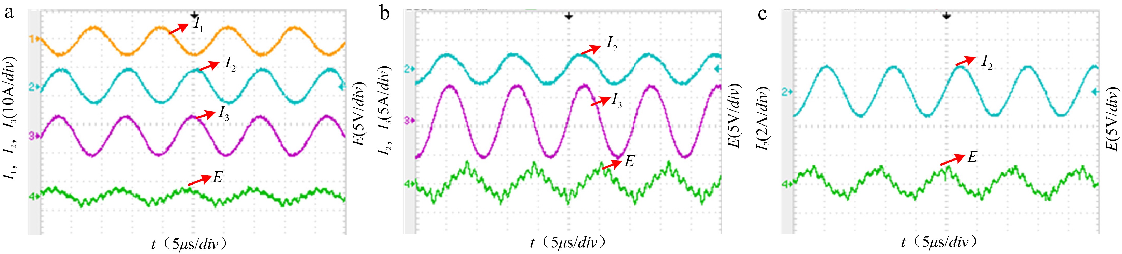
Figure 9. 

The experimental waveform diagram at different point.(a)Intersection.(b)Line midpoint.(c)Face centerpoint.

The magnitudes of the magnetic vector, corresponding to the induced voltages measured in the experiment and calculated via Eq. (23), are presented in Table 9.

As observed from Fig. 9 and Table 9, the spatial magnetic field magnitude of the centralized power transfer system can be effectively controlled to the desired value around 7 A/m at different field point locations using the proposed magnetic field control method. Despite minor discrepancies due to system parameters in accuracy and experimental measurement errors, the recorded errors at the three points are 7.6%, 6.7%, and 4.7%, all remaining within 10%. These results validate the correctness of applying the proposed magnetic energy steering method to the centralized power transfer system.

Experimental verification of distributed magnetic energy control principles

Following the optimal excitation current combination selected from Fig. 10 and due to the identical verification methodology, only the magnetic vector's X-direction orientation and magnitude are validated herein. The parameters of the optimal current combination from Table 7 are applied to the experimental platform in Fig. 7, with the resulting waveforms presented in Fig. 10.

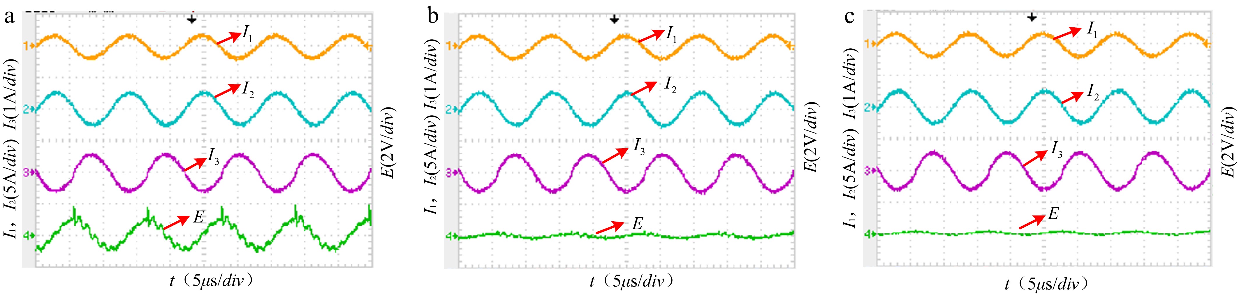
Figure 10. 

Experimental waveform plots of magnetic field components in the (a) X, (b) Y, and (c) Z directions at point M.

As observed from Fig. 10 and calculated using Eq. (23), the X-component of the magnetic field at point M is dominant at 6.5 A/m, while the Y- and Z-components are significantly smaller at 1.43 A/m and 1.28 A/m, respectively. This indicates that the magnetic field direction at point M is predominantly aligned with the positive X-direction. However, due to system parameter inaccuracies and experimental measurement errors, a deviation exists, with a measured error of 7.2% in the magnetic field magnitude along the desired direction. Overall, the theoretical, simulation, and experimental results are in good agreement, thereby validating the application of the proposed magnetic energy steering method to the distributed power transfer system.

Centralized and distributed effective distance verification

To conduct a comparative analysis of the effective power transfer ranges between centralized and distributed wireless power transfer systems under a given current threshold, the maximum achievable transmission distance satisfying the constraints is sequentially solved along different angular directions, with the center of the centralized architecture serving as the origin. Based on magnetic field control theory, with the current threshold set to 4 A (RMS) and the target magnetic field intensity set to 7 A/m, the coil current amplitude along each angular direction is calculated as the transmission distance is incrementally increased. The computation continues until the current in any coil reaches the threshold, at which point the corresponding distance is recorded as the maximum transmission distance for that direction. By aggregating the results from all angular directions, the complete spatial distribution of the system's effective power transfer range can be obtained.

Considering three-dimensional symmetry, measurement directions are selected in the xOy plane with an angular step of 30°. For the centralized architecture, only the 0° and 30° directions need to be measured to reflect its full-circumference symmetric characteristics. For the distributed architecture, based on its structural symmetry, six representative directions 0°, 30°, 60°, 90°, 270°, and 300° are chosen for analysis, as illustrated in Fig. 11.

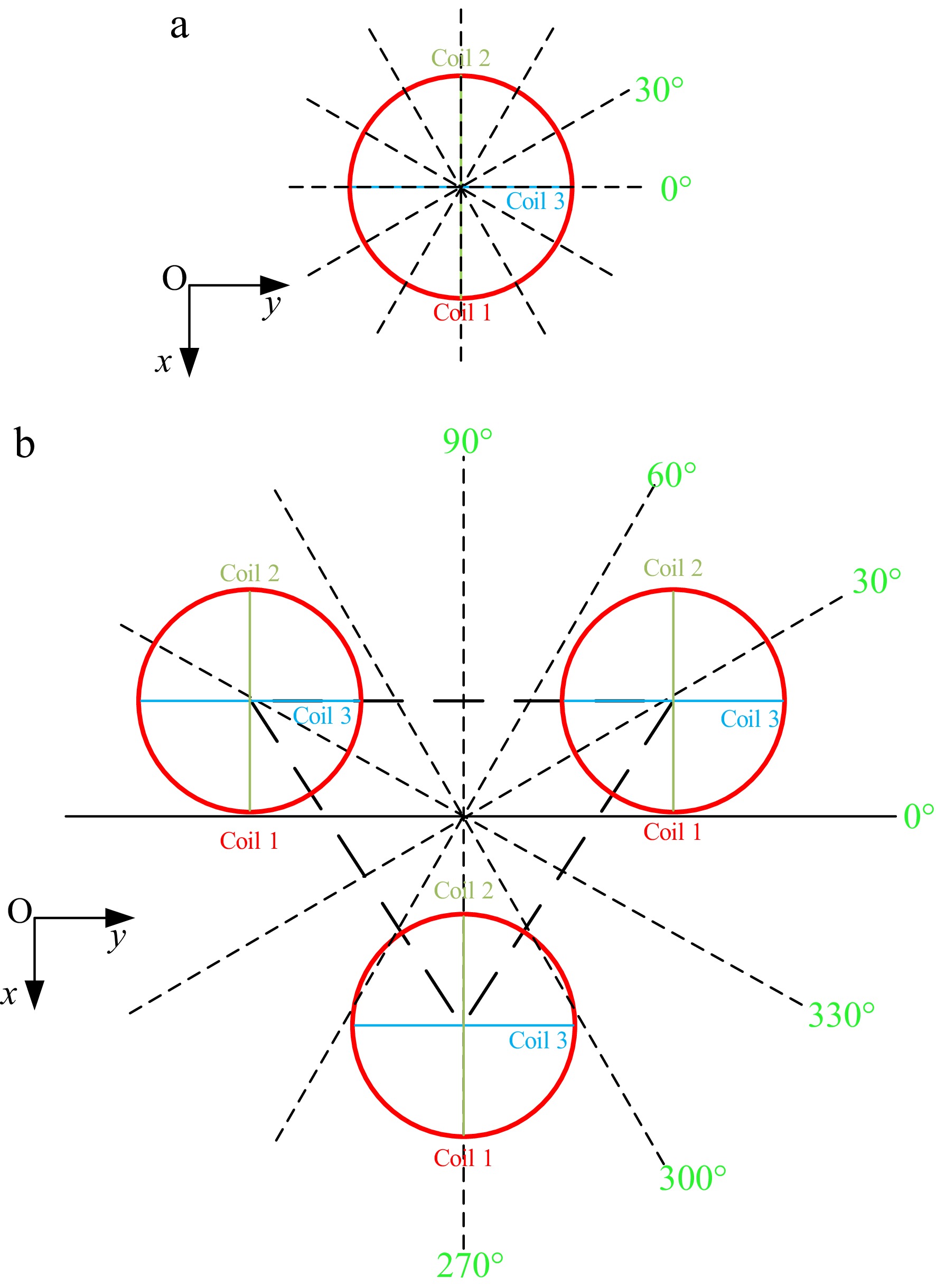
Figure 11. 

(a) Centralized and (b) distributed omnidirectional effective power transfer direction schematic diagram.

In the theoretical calculations, the maximum transmission distance at which the current threshold is reached in each direction, and the corresponding current distribution are recorded, with the results summarized in Tables 10 and 11. Since the measurement plane is positioned at the height of the node center, Coil 1 does not participate in excitation within the xOy plane. For directions where the threshold is not precisely reached during the stepwise distance increment, the final effective distance before the current first exceeds the threshold is taken as the maximum transmission distance in that direction.

In the experimental verification, the induced voltage corresponding to a magnetic field intensity of 7 A/m is 0.7 V. The parameters obtained from theoretical calculations for each direction are applied to the experimental platform. The measured waveforms are shown in Figs 12 and 13, and the actual maximum transmission distances are recorded. Fig. 14 comprehensively compares the maximum transmission distances of the centralized and distributed systems based on theoretical, simulation, and experimental results, thereby effectively validating the accuracy of the power transfer range.

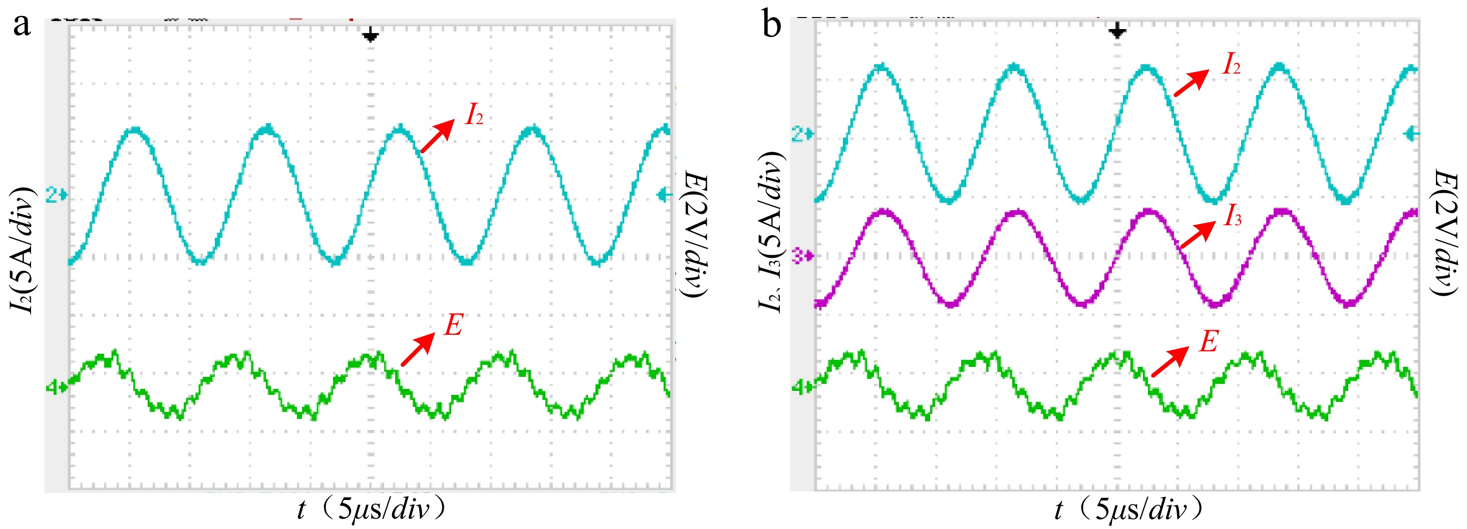
Figure 12. 

Waveform of the effective distance test for centralized magnetic energy control system (a) 0°. (b) 30°.

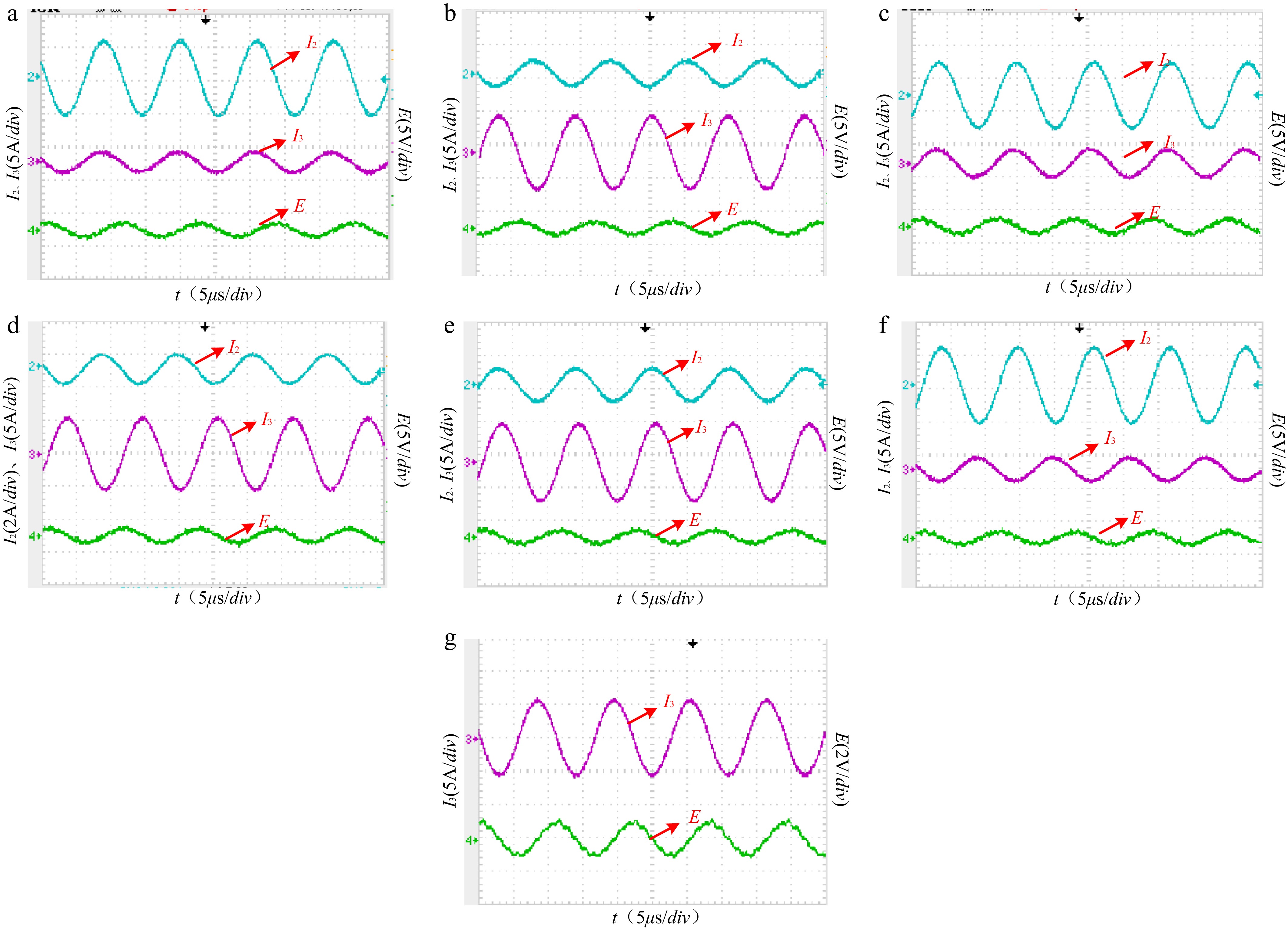
Figure 13. 

Waveform of the effective distance test for a distributed magnetic energy control system (a) 90°, (b) 60°, (c) 30°, (d) 0°, (e) 330°, (f) 300°, and (g) 270°.

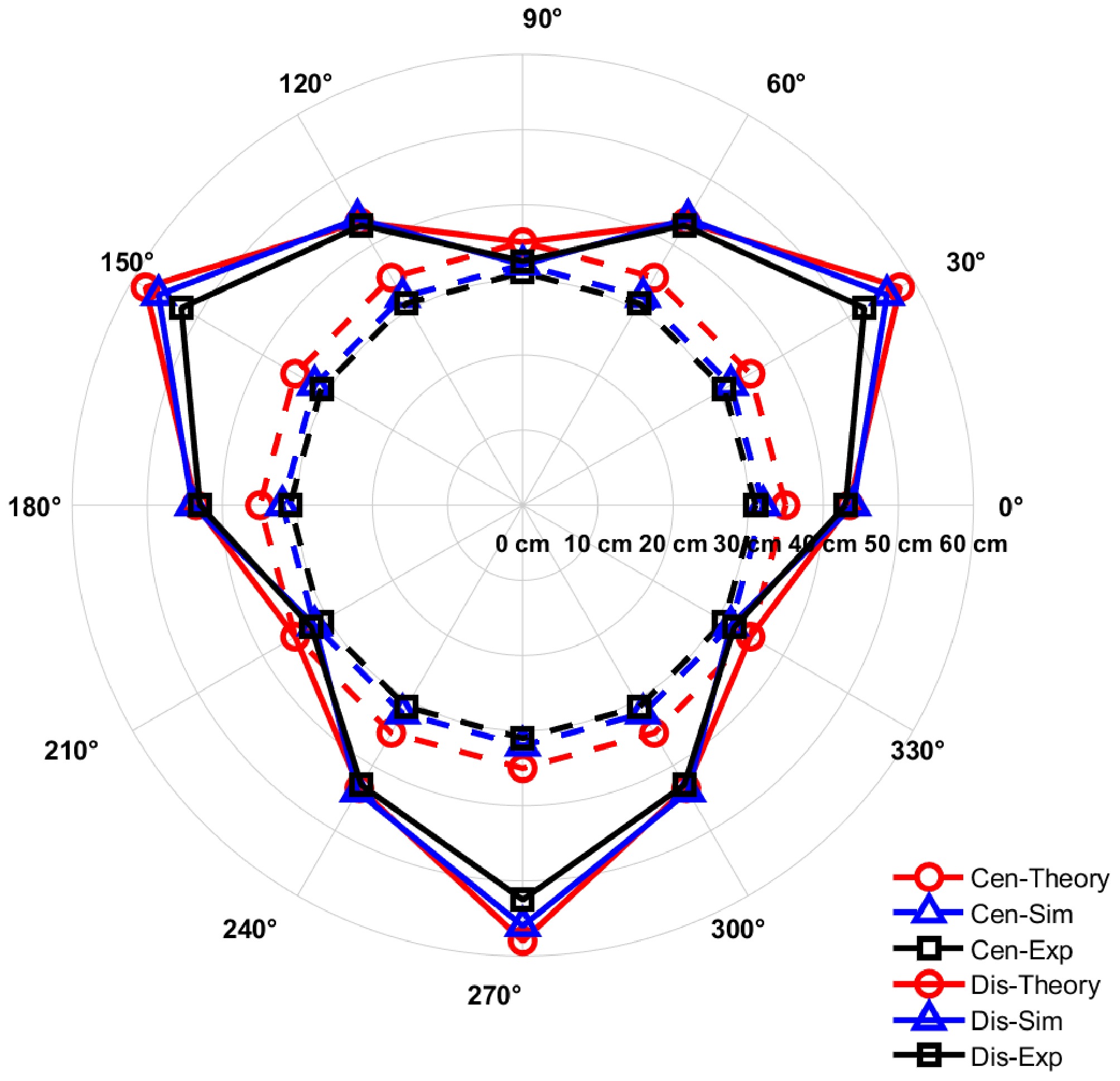
Figure 14. 

Effective distance distribution of centralized and distributed magnets.

The integrated theoretical and experimental results demonstrate that the proposed centralized and distributed magnetic energy control systems possess stable omnidirectional power transmission capability across the full-space range.

This paper introduces a novel framework designed to address the challenges of angular misalignment, limited spatial coverage, and power transfer dead zones. This framework incorporates both centralized and distributed 3D orthogonal transmission modalities. Central to this work is a proposed multi-excitation cooperative control strategy that leverages excitation current amplitude modulation for magnetic energy regulation. This strategy facilitates precise directional control of the magnetic field while simultaneously minimizing excitation source losses, leading to a substantial boost in transfer efficiency. The synergy between the proposed architecture and the control strategy empowers the system to manipulate the magnetic field vector at any arbitrary point within its effective domain, enabling the realization of omnidirectional, full-angle, low-leakage, and highly efficient power delivery with pinpoint accuracy.