











-
Multi-quadrotor unmanned aerial vehicles (UAVs) are defined by their multirotor actuation features and multiple degrees of freedom, which enable flexible trajectory tracking and agile attitude adjustment[1−3]. These capabilities make multi-quadrotor UAVs well suited for cooperative missions. Using cooperative control algorithms, multi-quadrotor UAV systems can accomplish swarm tasks, supporting applications such as load transportation[4], target surveillance[5], and search and strike[6]. When obstacle-free scenarios are considered, formation control can be addressed effectively. However, in practical mission scenarios, the spatial constraints imposed by complex three-dimensional (3D) obstacle environments tightly couple formation maintenance with obstacle avoidance. This poses challenges for conventional cooperative control algorithms in achieving both objectives simultaneously.
The main formation control strategies include virtual structure methods[7−9], behavior-based methods[10−12], and consensus algorithms[13−15]. Belkacem et al.[16] developed a distributed algorithm for achieving consensus tracking in second-order multiagent systems that avoids the chattering effect typically induced by traditional sliding-mode control protocols. Zhang et al.[17] framed a leader–follower cooperative guidance law via backstepping approach based on graph theoretic communication topology. Ollervides-Vazquez et al.[18] developed a sectorial fuzzy consensus approach for the formation flight of multi-quadrotor UAVs based on the Newton–Euler model and a sectorial fuzzy controller. Miao et al.[19] introduced a distributed formation control scheme that operates without requiring outer-loop linear velocity or inner-loop angular velocity measurements. In distributed formation control, individual coordination is strongly linked to collective behavior, with heavy reliance on cooperative error feedback and accurate system models. This reliance reduces flexibility and substantially complicates controller design as system complexity increases. Moreover, multifunctionality and scalability are often constrained by packaging limitations. Accordingly, Wang et al.[20] presented a hierarchical distributed control framework that decouples the problem into a reference generation layer and a tracking control layer. Furthermore, Wang et al.[21] investigated the consensus problem of second-order leader–follower systems with velocity constraints and developed a hierarchical constrained distributed control scheme.
Unknown obstacles in practical mission scenarios pose a critical challenge to the safety of cooperative formations. Consequently, various approaches have been proposed for obstacle avoidance, including graph search algorithms[22], genetic algorithms[23], and reinforcement learning methods[24]. Compared with the aforementioned methods, the artificial potential field (APF) method guides the agent by superimposing an attractive potential toward the goal and a repulsive potential away from obstacles, thereby generating an obstacle avoidance trajectory from the start to the goal[25]. As the APF method features structural simplicity, real-time implementability, and rapid responsiveness to environmental changes, it has been widely applied to collision avoidance[26−28] and obstacle avoidance[29−31]. Matoui et al.[32] developed a centralized APF-based planner to generate trajectories for multirobot systems that operate in dynamic environments. Hu et al.[33] reported an integrated approach that combines Voronoi partitions with a conventional APF to achieve distributed formation control and collision avoidance. To mitigate the inherent local minima and oscillatory behavior of conventional APF methods, Pan et al.[34] developed a hybrid formation control scheme by combining a rotational potential field with a leader–follower strategy, enabling follower UAVs to maintain prescribed relative angles and distances with respect to the leader. Huang et al.[35] introduced a parallel search strategy to mitigate the local minimum trap and goal inaccessibility problems that arise near obstacles in conventional APF methods. For dynamic obstacle avoidance, Wang et al.[36] modified the repulsive potential function and introduced an adaptive repulsion coefficient that depends on the obstacle velocity. Furthermore, Liu et al.[37] developed an improved repulsive force with a continuously differentiable regulation mechanism, which eliminates the influence of obstacles outside the detection range. Despite the proven feasibility of existing formation obstacle avoidance methods, the limited flexibility of traditional distributed control frameworks poses a challenge.
Inspired by the aforementioned research, this paper proposes a hierarchical distributed formation obstacle avoidance control scheme for multi-quadrotor UAVs in 3D obstacle environments. The proposed design consists of three steps. First, to cope with the increased collision risks induced by 3D obstacles during formation maneuvering, the formation is enclosed by a virtual sphere whose center is the virtual leader, and an adaptive artificial potential field (AAPF)-based planner is used to generate an obstacle avoidance trajectory for this sphere so that the entire formation can pass through cluttered spaces safely. Second, a distributed reference signal generator is designed to maintain the desired formation configuration and produce obstacle avoidance reference trajectories for the multi-quadrotor UAVs by embedding the virtual leader's planned trajectory. Finally, the generator outputs are taken as the reference trajectories for each multi-quadrotor UAV, and extended state observer (ESO)-based composite controllers are designed to achieve trajectory tracking under conditions of disturbances and uncertainties. The main contributions of this paper are twofold:
1. By incorporating an adaptive gain mechanism into the repulsive force, the proposed AAPF method alleviates oscillations near the obstacle avoidance boundary that commonly arise in traditional APF schemes. This design reduces sensitivity to gain tuning and enhances adaptability across different scenarios.
2. The proposed control scheme decouples the traditional distributed formation obstacle avoidance problem into a two layer structure, based on the virtual leader's obstacle avoidance trajectory planned by the AAPF method. This hierarchical framework improves the flexibility and robustness of the system design.
The rest of this paper is organized as follows. Section “Preliminaries and problem formulation” provides the preliminaries and formulates the problem. Section “Main Results” develops a hierarchical distributed formation obstacle avoidance control scheme for multi-quadrotor UAV systems. Section “Experiments” reports experimental validations and discusses the results. Finally, some conclusions are drawn in Section “Conclusions”.
-
Notations:
$ \mathbb{R}^n $ $ n $ $ \mathbb{R}^{n\times m} $ $ n\times m $ $ {\bf{0}}_m=[0,\ldots,0]^T\in\mathbb{R}^m $ $ {\bf{0}}_{n\times m}\in\mathbb{R}^{n\times m} $ $ {I}_n \in \mathbb{R}^{n \times n} $ $ n \times n $ $ A\in\mathbb{R}^{n\times n} $ $ \lambda_{\min}(A) $ $ \lambda_{\max}(A) $ $ \|\cdot\|_2 $ $ {\boldsymbol{P}} \in \mathbb{R}^{n \times n} $ $ {\boldsymbol{x}} \in \mathbb{R}^n $ $ \lambda_{\min}({\boldsymbol{P}})\|{\boldsymbol{x}}\|_2^2 \le {{\boldsymbol{x}}^T {\boldsymbol{P}} {\boldsymbol{x}}} \le \lambda_{\max}({\boldsymbol{P}})\|{\boldsymbol{x}}\|_2^2 $ Graph theory notions
-
For the leader–follower case, node
$ 0 $ $ 1,\ldots,N $ $ G = ({\cal{V}}, {\cal{E}}, {\cal{A}}) $ $ {\cal{V}} = \{1, \ldots, N\} $ $ {\cal{E}} \subseteq {\cal{V}} \times {\cal{V}} $ $ {\cal{A}} = [a_{ij}] \in \mathbb{R}^{N \times N} $ $ a_{ij} = a_{ji} \gt 0 $ $ (j, i) \in {\cal{E}} $ $ a_{ij} = 0 $ $ a_{ii} = 0, \forall i \in {\cal{V}} $ $ i $ $ {\cal{N}}_i = \{j \in {\cal{V}} \mid (j,i) \in {\cal{E}}\} $ $ G $ $ L = [l_{ij}] \in \mathbb{R}^{N \times N} $ $ l_{ii} = \sum_{j \in {\cal{N}}_i} a_{ij} $ $ l_{ij} = -a_{ij} $ $ i \neq j $ $ \bar{G} $ $ \bar{{\cal{V}}} = \{0\} \cup {\cal{V}} $ $ i $ $ b_i $ $ b_i \gt 0 $ $ b_i = 0 $ $ B = \text{diag}\{b_1, \ldots, b_N\} $ $ M = L + B $ Useful lemmas
-
Lemma 1. If a directed graph
$ \bar{G} $ $ B \neq 0 $ $ M $ Lemma 2. Let
$ x, y \in \mathbb{R} $ $ \varkappa \gt 0 $ $ p \gt 1 $ $ q \gt 1 $ $ (p - 1)(q - 1) = 1 $ $ xy $ $ xy \leq \dfrac{\varkappa^p}{p} |x|^p + \dfrac{1}{q \varkappa^q} |y|^q $ Definition 1. Consider the system
$ \dot{x}=f(t,x,u) $ $ f:[0,+\infty)\times \mathbb{R}^n\times \mathbb{R}^m\to\mathbb{R}^n $ $ t $ $ x $ $ u $ $ u(t) $ $ t $ $ t\ge 0 $ $ \dot{x}=f(t,x,u) $ $ {\cal{K}}{\cal{L}} $ $ \beta(\cdot,\cdot) $ $ {\cal{K}} $ $ \gamma(\cdot) $ $ x(t_0) $ $ u(t) $ $ x(t) $ $ \forall t \geq t_0 $ $ \|x(t)\|_2 \le \beta\big(\|x(t_0)\|_2, \,t-t_0\big) + \gamma \left(\sup_{t_0\le \tau \le t}\|u(\tau)\|_2\right) $ Lemma 3. Suppose
$ f $ $ (x,u) $ $ t $ $ \dot{x}=f(t,x,{\bf{0}}_m) $ System modeling and problem formulation
System modeling
-
A team of
$ N $ $ {\cal{F_e}}=\{O_e,X_e,Y_e,Z_e\} $ $ O_e $ $ O_eX_e $ $ O_eZ_e $ $ O_eY_e $ $ {\cal{F_b}}=\{O_b,X_b,Y_b,Z_b\} $ $ O_b $ $ O_bX_b $ $ O_bZ_b $ $ O_bY_b $ $ O_bZ_b $ $ O_bX_b $ $ O_bY_b $ $ O_bZ_b $ The communication among the multi-quadrotor UAVs is described by an undirected graph
$ G=({\cal{V}},{\cal{E}},{\cal{A}}) $ $ {\cal{V}}=\{1,\ldots,N\} $ $ {\cal{E}} \subseteq\cal{V}\times{\cal{V}} $ $ {\cal{A}}=[a_{ij}] $ $ (j,i)\in{\cal{E}} $ $ i $ $ j $ $ i $ $\mathcal N_i=\{j\in\mathcal V\mid (j,i)\in\mathcal E\}$ $ \bar G $ $ \bar{{\cal{V}}}=\{0\}\cup{\cal{V}} $ $ 0 $ $ i\in{\cal{V}} $ $ \bar G $ The inner–outer-loop structure is employed to facilitate controller design for the multi-quadrotor UAVs. The outer (position) loop generates the desired thrust and attitude commands for the inner loop. The inner (attitude) loop, typically implemented by an onboard proportional–integral–derivative (PID) module, ensures fast attitude stabilization and tracking. This cascaded architecture enables outer-loop trajectory tracking for formation and obstacle avoidance tasks while preserving the fast response and robustness of the inner-loop attitude dynamics. The position loop model of the
$ i $ $ \ddot{{\boldsymbol{q}}}_i ={\boldsymbol{R}}_i \frac{{\boldsymbol{F}}_{bi}}{m_i}- {\boldsymbol{G}} + {\boldsymbol{d}}^p_i,\; i\in{\cal{V}}. $ (1) where
$ \ddot{\boldsymbol{q}}_i=[\ddot{x}_i,\ddot{y}_i,\ddot{z}_i]\mathrm{^T} $ $ {\cal{F_e}} $ $ \boldsymbol{q}_i=[x_i,y_i,z_i]\mathrm{^T} $ $ i $ $ {\cal{F_e}} $ $ {\cal{F_b}} $ $ \boldsymbol{F}_{bi}=[0,0,F_i]\mathrm{^T} $ $ F_i $ $ O_b Z_b $ $ m_i $ $ i $ $ \boldsymbol{G}=[0,0,g]\mathrm{^T} $ $ {\boldsymbol{d}}_i^{p}\in\mathbb{R}^3 $ $ {\boldsymbol{R_i}} $ $ \cal{F_b} $ $ \cal{F_e} $ $ {\boldsymbol{R}}_i= \left[\begin{array}{*{20}{c}} { c\theta_i c\psi_i }&{ c\psi_i s\theta_i s\phi_i - s\psi_i c\phi_i }&{ c\psi_i s\theta_i c\phi_i + s\psi_i s\phi_i }\\{ c\theta_i s\psi_i }&{ s\psi_i s\theta_i s\phi_i + c\psi_i c\phi_i }&{ s\psi_i s\theta_i c\phi_i - c\psi_i s\phi_i }\\{ -s\theta_i }&{ s\phi_i c\theta_i }&{ c\phi_i c\theta_i } \end{array}\right],\; i\in{\cal{V}}. $ (2) where
$ c \triangleq \cos $ $ s \triangleq \sin $ $ \phi_i $ $ \theta_i $ $ \psi_i $ $ i $ To address the underactuation of the position subsystem, the virtual control input
$ {\boldsymbol{u}}_i = {\boldsymbol{R}}_i\dfrac{{\boldsymbol{F}}_{bi}}{m_i} $ $ \boldsymbol{u}_i=[u_{xi},u_{yi},u_{zi}]\mathrm{^T} $ $ i \in{\cal{V}} $ $ i $ $ \begin{aligned} \dot{{\boldsymbol{q}}}_i &= {\boldsymbol{v}}_i,\\ \dot{{\boldsymbol{v}}}_i &= {\boldsymbol{u}}_i - {\boldsymbol{G}} + {\boldsymbol{d}}^p_i,\; i\in{\cal{V}}. \end{aligned} $ (3) The Euler-angle kinematics satisfy
$ \dot{{\boldsymbol{\Theta}}}_i={\boldsymbol{T}}({\boldsymbol{\Theta}}_i){\boldsymbol{\omega}}_i $ $ \boldsymbol{\Theta}_i=[\phi_i,\theta_i,\psi_i]\mathrm{^T} $ $ \dot{\boldsymbol{\Theta}}_i=[\dot{\phi}_i,\dot{\theta}_i,\dot{\psi}_i]^{\mathrm{T}} $ $ \boldsymbol{\omega}_i=[\omega_{x_i},\omega_{y_i},\omega_{z_i}]\mathrm{^T} $ $ {\cal{F_b}} $ $ {\boldsymbol{T}}({\boldsymbol{\Theta}}_i) $ $ {\boldsymbol{T}}({\boldsymbol{\Theta}}_i) = \left[\begin{array}{*{20}{c}} {1 }&{ t\theta_i s\phi_i }&{ t\theta_i c\phi_i }\\{ 0 }&{ c\phi_i }&{ -s\phi_i }\\{ 0 }&{ \dfrac{s\phi_i}{c\theta_i} }&{ \dfrac{c\phi_i}{c\theta_i} }\end{array}\right],\; i\in{\cal{V}}. $ (4) where
$ c \triangleq \cos $ $ s \triangleq \sin $ $ t \triangleq \tan $ The attitude dynamics of the
$ i $ $ J_i \dot{{\boldsymbol{\omega}}}_i + {\boldsymbol{\omega}}_i \times (J_i {\boldsymbol{\omega}}_i) = {\boldsymbol{\tau}}_i + {\boldsymbol{d}}^{a}_{i},\; i\in{\cal{V}}. $ (5) where
$ J_i = \text{diag}\{ J_{xx_i}, J_{yy_i}, J_{zz_i} \} $ $ \boldsymbol{\tau}_i=[\tau_{x_i},\tau_{y_i},\tau_{z_i}]\mathrm{^T} $ $ {\cal{F_b}} $ $ \boldsymbol{d}_i^a=[d_i^{\phi},d_i^{\theta},d_i^{\psi}]\mathrm{^T} $ Remark 1. The obstacle is modeled in the inertial-reference frame
$ {\cal{F_e}} $ $ {\boldsymbol{c}}=[x_c,y_c,z_c]^{\rm{T}}\in\mathbb{R}^3 $ $ z_c=0 $ $ r_o>0 $ $ h_o>0 $ Problem formulation
-
A team of
$ N $ $ {\cal{V}}=\{1,\ldots,N\} $ $ \dot{{\boldsymbol{q}}}_0={\boldsymbol{v}}_0 $ (6) where
$ {\boldsymbol{q}}_0=\big[x_0,\,y_0,\,z_0\big]^{\rm{T}}\in\mathbb{R}^3 $ $ {\boldsymbol{v}}_0=\big[v_{x0},\,v_{y0},\,v_{z0}\big]^{\rm{T}}\in\mathbb{R}^3 $ $ {\boldsymbol{v}}_0 $ Conventional schemes enforce formation coordination directly on the states of the multi-quadrotor UAVs, thereby coupling coordination with tracking transients and uncertainties. A distributed reference signal generator is developed over a network of second-order virtual agents to decouple reference generation from tracking. The virtual agent network inherits the communication topology of the multi-quadrotor UAV system. Through local information exchanges, it propagates the leader reference and generates reference signals for all multi-quadrotor UAVs. The dynamics of the virtual agent are formulated as
$ \begin{aligned} \dot{{\boldsymbol{q}}}_i^* &= {\boldsymbol{v}}_i^*,\\ \dot{{\boldsymbol{v}}}_i^* &= {\boldsymbol{u}}_i^*,\; i\in{\cal{V}}. \end{aligned} $ (7) where
$ {\boldsymbol{u}}_i^*=[u_{xi}^*,\,u_{yi}^*,\,u_{zi}^*]^{\rm{T}}\in\mathbb{R}^3 $ $ \boldsymbol{q}_i^*=[x_i^*,\, y_i^*,\, z_i^*]\mathrm{^T} $ $ \boldsymbol{v}_i^*=[v_{xi}^*,\, v_{yi}^*,\, v_{zi}^*]\mathrm{^T} $ $ i $ The objective is to guide the multi-quadrotor UAV formation from a given initial position to a desired goal in a 3D obstacle environment while maintaining the prescribed formation configuration and ensuring obstacle avoidance. A hierarchical distributed formation obstacle avoidance control scheme is proposed, as depicted in Fig. 1. At the reference signal generation layer, an AAPF-based planner generates a 3D obstacle avoidance trajectory for the virtual leader
$ {\boldsymbol{q}}_0 $ $ d_{{\rm{obs}}}({\boldsymbol{q}}_0)=\|{\boldsymbol{q}}_0- $ $ {\boldsymbol{q}}_{{\rm{obs}}}({\boldsymbol{q}}_0)\|_2- r_{{o}}-r_{ f}>0 $ $ {\cal{B}}({\boldsymbol{q}}_0,r_{ f}) $ $ {\boldsymbol{q}}_0 $ $ \|{\boldsymbol{q}}_i-{\boldsymbol{q}}_0\|_2 \le r_{ f} $ $ r_{ f}=\max_{i\in{\cal{V}}}\|{\boldsymbol{q}}_i-{\boldsymbol{q}}_0\|_2 $ $ ({\boldsymbol{q}}_0,{\boldsymbol{v}}_0) $ $ {\boldsymbol{h}}_i=\big[h_{xi},h_{yi},h_{zi}\big]^{\rm{T}} $ $ i $ $ \lim_{t\to+\infty}\|{\boldsymbol{q}}_i^*(t)-{\boldsymbol{q}}_0(t)-{\boldsymbol{h}}_i\|_2=0 $ $ \lim_{t\to+\infty}\|{\boldsymbol{v}}_i^*(t)-{\boldsymbol{v}}_0(t)\|_2= 0 $ 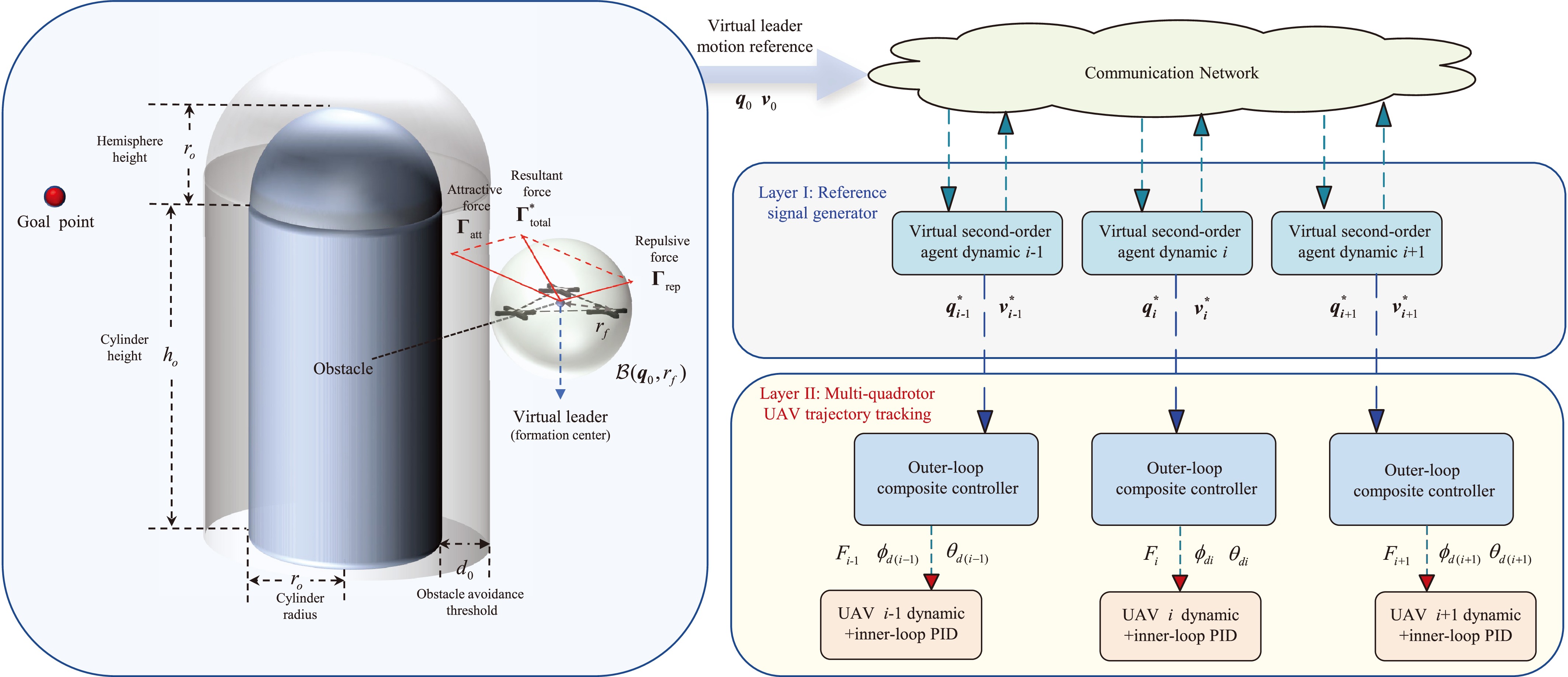
Figure 1.
Block diagram of the hierarchical distributed formation obstacle avoidance control scheme.
-
The AAPF method is utilized for 3D motion planning. The goal generates an attractive potential, whereas obstacles generate repulsive potentials. Formation-level safety is enforced by enclosing the formation within a safety sphere and activating the repulsive action when the sphere-obstacle clearance falls below a prescribed obstacle avoidance threshold. The virtual leader advances in the direction of the resultant force, guiding the formation toward the target while avoiding obstacles.
Attractive field and force design
-
The attractive potential is expressed as[25]
$ U_{{\rm{att}}}({\boldsymbol{q}}_0) =\frac{1}{2}K_{{\rm{att}}}\; d_{{\rm{goal}}}^{2}({\boldsymbol{q}}_0,{\boldsymbol{q}}_{{\rm{goal}}}) $ (8) where
$ {\boldsymbol{q}}_0 $ $ \boldsymbol{q}_{\rm{goal}}= [x_g,\, y_g,\, z_g]^{\mathrm{T}} $ $ d_{{\rm{goal}}}({\boldsymbol{q}}_0,{\boldsymbol{q}}_{{\rm{goal}}})=\|{\boldsymbol{q}}_0-{\boldsymbol{q}}_{{\rm{goal}}}\|_2 $ $ K_{{\rm{att}}}>0 $ The attractive force is given by
$ \begin{align} {\boldsymbol{\Gamma}}_{{\rm{att}}}({\boldsymbol{q}}_0) &= -\nabla U_{{\rm{att}}}({\boldsymbol{q}}_0) \\ &= -K_{{\rm{att}}} \big({\boldsymbol{q}}_0 - {\boldsymbol{q}}_{{\rm{goal}}}\big) . \end{align} $ (9) Repulsive field and force design
-
The equivalent obstacle center
$ {\boldsymbol{q}}_{{\rm{obs}}}({\boldsymbol{q}}_0) $ $ {\boldsymbol{q}}_0 $ $ \boldsymbol{q}_{\rm{obs}}(\boldsymbol{q}_0)=\left\{\begin{array}{*{20}{l}}[x_c,\, y_c,\, z_0]^{\mathrm{T}}, & z_0\le z_c+h_o\ , \\ \boldsymbol{c}+[0,0,h_o]\mathrm{^T,} & z_0 \gt z_c+h_o\ ,\end{array}\right. $ (10) where
$ z_0 $ $ h_o $ $ {\boldsymbol{c}}=[x_c,y_c,z_c]^{\rm{T}}\in\mathbb{R}^3 $ The repulsive term is activated when the formation-enclosing sphere enters the obstacle-avoidance region. Therefore, the repulsive potential is defined as
$ U_{\rm{rep}}(\boldsymbol{q}_0)=\left\{\begin{array}{*{20}{l}}\dfrac{1}{2} \left(\dfrac{1}{d_{\rm{obs}}(\boldsymbol{q}_0)}-\dfrac{1}{d_0}\right)^2, & d_{\rm{obs}}(\boldsymbol{q}_0)\le d_0\ , \\ 0, & d_{\rm{obs}}(\boldsymbol{q}_0) \gt d_{0\ },\ \end{array}\right. $ (11) where
$ d_0>0 $ $ d_{{\rm{obs}}}({\boldsymbol{q}}_0)\le d_0 $ Remark 2. The 3D obstacle avoidance is implemented at the formation level by enclosing the multi-quadrotor UAV formation within
$ {\cal{B}}({\boldsymbol{q}}_0,r_f) $ $ z_c=0 $ $ [x_c,\, y_c,\, z_0]\mathrm{^T} $ $ z_0 \le h_o $ $ [x_c,\, y_c,\, h_o]\mathrm{^T} $ $ z_0 \gt h_o $ The repulsive gain is adaptively adjusted as a distance-dependent function:
$ K_{{\rm{rep}}}^*= \left\{\begin{array}{*{20}{l}} { K_{{\rm{rep}}}^{\min}+\Delta K_{{\rm{rep}}} \left(1-\dfrac{d_{{\rm{obs}}}({\boldsymbol{q}}_0)}{d_0}\right),} & {d_{{\rm{obs}}}({\boldsymbol{q}}_0)\le d_0,}\\ {0, }& {d_{{\rm{obs}}}({\boldsymbol{q}}_0) \gt d_0.} \end{array}\right. $ (12) where
$ \Delta K_{{\rm{rep}}}=K_{{\rm{rep}}}^{\max}-K_{{\rm{rep}}}^{\min} $ $ K_{{\rm{rep}}}^{\min} $ $ K_{{\rm{rep}}}^{\max} $ The repulsive force is given by
$ \begin{align} {\boldsymbol{\Gamma}}_{{\rm{rep}}}({\boldsymbol{q}}_0) &= -K_{{\rm{rep}}}^{*}\nabla U_{{\rm{rep}}}({\boldsymbol{q}}_0)\\ &= \left\{\begin{array}{*{20}{l}} {K_{{\rm{rep}}}^{*}\,\dfrac{1}{d_{{\rm{obs}}}^{2}({\boldsymbol{q}}_0)}\left(\dfrac{1}{d_{{\rm{obs}}}({\boldsymbol{q}}_0)}-\dfrac{1}{d_0}\right)\,\dfrac{\partial d_{{\rm{obs}}}({\boldsymbol{q}}_0)}{\partial {\boldsymbol{q}}_0}, }& {d_{{\rm{obs}}}({\boldsymbol{q}}_0)\le d_0,}\\{ 0, }&{ d_{{\rm{obs}}}({\boldsymbol{q}}_0) \gt d_0. } \end{array}\right. \end{align} $ (13) Remark 3. The repulsive gain is adjusted linearly between
$ K_{\text{rep}}^{\text{min}} $ $ K_{\text{rep}}^{\text{max}} $ $ d_{{\rm{obs}}}({\boldsymbol{q}}_0) $ $ d_0 $ $ 0 $ $ K_{\text{rep}}^{*} $ $ K_{\text{rep}}^{\text{min}} $ $ K_{\text{rep}}^{\text{max}} $ Accordingly, the resultant force is computed as
$ {\boldsymbol{\Gamma}}_{{\rm{total}}}^{*}({\boldsymbol{q}}_0) = {\boldsymbol{\Gamma}}_{{\rm{att}}}({\boldsymbol{q}}_0) + {\boldsymbol{\Gamma}}_{{\rm{rep}}}({\boldsymbol{q}}_0) $ (14) Remark 4. In the traditional APF method, a fixed repulsive gain is typically selected. When the repulsive gain is chosen inappropriately, it may cause overly aggressive avoidance maneuvers near the safety boundary or result in an insufficient avoidance response, thereby increasing the risk of collision. Therefore, an adaptive repulsive gain mechanism is introduced, which reduces sensitivity to parameter tuning and mitigates chattering in the repulsive force.
Distributed reference signal generator design
-
The virtual leader's control input is obtained from the resultant force generated by the AAPF method:
$ \begin{align} \dot{{\boldsymbol{q}}}_0 &= {\boldsymbol{v}}_{0} \\ &= {\boldsymbol{\Gamma}}^*_{\text{total}}({\boldsymbol{q}}_0) \end{align} $ (15) where
$ {\boldsymbol{q}}_0=[x_0,y_0,z_0]^T\in\mathbb{R}^3 $ $ {\boldsymbol{v}}_0=[v_{x0},v_{y0},v_{z0}]^T\in\mathbb{R}^3 $ Remark 5. The obstacle avoidance trajectory is generated by planning the motion of the virtual leader
$ {\boldsymbol{q}}_0 $ $ {\boldsymbol{\Gamma}}^*_{{\rm{total}}}({\boldsymbol{q}}_0) $ $ d_{{\rm{obs}}}({\boldsymbol{q}}_0) $ $ d_0 $ Assumption 1. The virtual leader reference trajectory generated by the AAPF method is admissible (i.e., feasible for implementation). For analytical tractability, the virtual leader velocity is idealized as a constant vector in the subsequent stability analysis, i.e.,
$ \dot{{\boldsymbol{v}}}_0(t)={\bf{0}}_3 $ The distributed reference signal generator produces the formation obstacle avoidance reference trajectories for the multi-quadrotor UAVs as
$ \dot{{\boldsymbol{q}}}_i^* = {\boldsymbol{v}}_i^* -\mu_1 \left\{ \sum\limits_{j \in {\cal{N}}_i} a_{ij} \left[ ({\boldsymbol{q}}_i^*-{\boldsymbol{h}}_i) -({\boldsymbol{q}}_j^*-{\boldsymbol{h}}_j) \right] + b_i \left[ {\boldsymbol{q}}_i^*-({\boldsymbol{q}}_0+{\boldsymbol{h}}_i) \right] \right\}, $ (16) $ \dot{{\boldsymbol{v}}}_i^* = -\mu_2 \left[ \sum\limits_{j \in {\cal{N}}_i} a_{ij} \left( {\boldsymbol{v}}_i^*-{\boldsymbol{v}}_j^* \right) + b_i \left( {\boldsymbol{v}}_i^*-{\boldsymbol{v}}_0 \right) \right],\; i\in{\cal{V}}. $ (17) where
$ {\boldsymbol{q}}_i^*=[x_i^*,y_i^*,z_i^*]^T\in\mathbb{R}^3 $ $ {\boldsymbol{v}}_i^*=[v_{xi}^*,v_{yi}^*,v_{zi}^*]^T\in\mathbb{R}^3 $ $ \mu_1,\mu_2>0 $ $ {\boldsymbol{h}}_i\in\mathbb{R}^3 $ $ {\boldsymbol{h}}_j\in\mathbb{R}^3 $ $ i $ $ j $ The formation tracking errors of the generator are defined as
$ \begin{aligned} \tilde{{\boldsymbol{q}}}_i &= {\boldsymbol{q}}_i^* - ({\boldsymbol{q}}_0 + {\boldsymbol{h}}_i), \\ \tilde{{\boldsymbol{v}}}_i &= {\boldsymbol{v}}_i^* - {\boldsymbol{v}}_0,\; i\in{\cal{V}}. \end{aligned} $ (18) Based on Eqs. (16)–(18), the formation tracking error system is
$ \begin{aligned} \dot{\tilde{{\boldsymbol{q}}}}_i &= \tilde{{\boldsymbol{v}}}_i -\mu_1 \left[ \sum_{j \in {\cal{N}}_i} a_{ij}\left(\tilde{{\boldsymbol{q}}}_i-\tilde{{\boldsymbol{q}}}_j\right) + b_i \tilde{{\boldsymbol{q}}}_i \right],\\ \dot{\tilde{{\boldsymbol{v}}}}_i &= -\mu_2 \left[ \sum_{j \in {\cal{N}}_i} a_{ij}\left(\tilde{{\boldsymbol{v}}}_i-\tilde{{\boldsymbol{v}}}_j\right) + b_i \tilde{{\boldsymbol{v}}}_i \right],\; i\in{\cal{V}}. \end{aligned} $ (19) As the
$ x $ $ y $ $ z $ $ \begin{aligned} \dot{\tilde{{\boldsymbol{q}}}} &= \tilde{{\boldsymbol{v}}} - \mu_1 M \tilde{{\boldsymbol{q}}},\\ \dot{\tilde{{\boldsymbol{v}}}} &= -\mu_2 M \tilde{{\boldsymbol{v}}}. \end{aligned} $ (20) where
$ \tilde{{\boldsymbol{q}}} = [\tilde{{q}}_1, \dots, \tilde{{q}}_N]^T \in \mathbb{R}^{N} $ $ \tilde{{\boldsymbol{v}}} = [\tilde{{v}}_1, \dots, \tilde{{v}}_N]^T \in \mathbb{R}^{N} $ Proposition 1. If Assumption 1 is satisfied, the origin of the error dynamics associated with the distributed reference signal generator given by Eqs (16) and (17) is exponentially stable. The formation position and velocity tracking errors satisfy
$ \lim_{t\to+\infty}\tilde{{\boldsymbol{q}}}(t)={\bf{0}}_N $ $ \lim_{t\to+\infty}\tilde{{\boldsymbol{v}}}(t)={\bf{0}}_N $ $ i\in{\cal{V}} $ $ \lim_{t\to+\infty}\big\|{\boldsymbol{q}}_i^{*}(t)-{\boldsymbol{q}}_0(t)-{\boldsymbol{h}}_i\big\|_2=0 $ $ \lim_{t\to+\infty}\left\|{\boldsymbol{v}}_i^{*}(t)-{\boldsymbol{v}}_0(t)\right\|_2=0 $ $ t\to+\infty $ Proof. The formation tracking error dynamics in Eq. (20) can be expressed in the following compact form:
$ \left[\begin{array}{*{20}{c}} \dot{\tilde{{\boldsymbol{q}}}}\\ \dot{\tilde{{\boldsymbol{v}}}} \end{array}\right] = \left[\begin{array}{*{20}{c}} {-\mu_1 M} &{ I_N}\\ { {\bf{0}}_{N\times N} }& {-\mu_2 M } \end{array}\right] \left[\begin{array}{*{20}{c}} \tilde{{\boldsymbol{q}}}\\ \tilde{{\boldsymbol{v}}} \end{array}\right]= D \left[\begin{array}{*{20}{c}} \tilde{{\boldsymbol{q}}}\\ \tilde{{\boldsymbol{v}}} \end{array}\right] $ (21) The augmented error state is defined as
$ {\boldsymbol{\delta}}=\left[\begin{array}{*{20}{c}}\tilde{{\boldsymbol{q}}}^{\rm{T}}, \tilde{{\boldsymbol{v}}}^{\rm{T}}\end{array}\right]^{\rm{T}}\in \mathbb{R}^{2N} $ $ \dot{{\boldsymbol{\delta}}}=D{\boldsymbol{\delta}} $ $ D\in\mathbb{R}^{2N\times 2N} $ $ \mu_1>0 $ $ \mu_2>0 $ $ D $ $ Q_f\in\mathbb{R}^{2N\times 2N} $ $ P_f\in\mathbb{R}^{2N\times 2N} $ $ D^{T}P_f + P_fD = -Q_f $ (22) The Lyapunov function is given by
$ V_f={\boldsymbol{\delta}}^T P_f {\boldsymbol{\delta}} $ (23) Taking the time derivative of Eq. (23) yields
$ \begin{align} \dot V_f &= \dot{{\boldsymbol{\delta}}}^T P_f {\boldsymbol{\delta}} + {\boldsymbol{\delta}}^T P_f \dot{{\boldsymbol{\delta}}} \\ &= -{\boldsymbol{\delta}}^T Q_f {\boldsymbol{\delta}} \\ &\le -\lambda_{\min}(Q_f)\|{\boldsymbol{\delta}}\|_2^2 \end{align} $ (24) From Eq. (24) and
$ \lambda_{\min}(P_f)\|{\boldsymbol{\delta}}\|_2^2\leq V_f \le \lambda_{\max}(P_f)\|{\boldsymbol{\delta}}\|_2^2 $ $ \begin{align} \dot V_f &\le -\frac{\lambda_{\min}(Q_f)}{\lambda_{\max}(P_f)}\,V_f\\ &=-\kappa\,V_f \end{align} $ (25) where
$ \kappa=\dfrac{\lambda_{\min}(Q_f)}{\lambda_{\max}(P_f)}>0 $ $ V_f(t) $ $ V_f(t)\le V_f(0)e^{-\kappa t} $ $ \forall t\ge 0 $ $ \tilde{{\boldsymbol{q}}}(t) $ $ {\bf{0}}_N $ $ \lim_{t\to+\infty}\tilde{{\boldsymbol{q}}}(t)={\bf{0}}_N $ $ \lim_{t\to+\infty}\left\|{\boldsymbol{q}}_i^{*}(t)-{\boldsymbol{q}}_0(t)-{\boldsymbol{h}}_i\right\|_2=0 $ $ i\in{\cal{V}} $ $ \tilde{{\boldsymbol{v}}}(t) $ $ {\bf{0}}_N $ $ \lim_{t\to+\infty}\tilde{{\boldsymbol{v}}}(t)={\bf{0}}_N $ $ \lim_{t\to+\infty}\left\|{\boldsymbol{v}}_i^{*}(t)-{\boldsymbol{v}}_0(t)\right\|_2=0 $ $ i\in{\cal{V}} $ □ Multi-quadrotor UAVs trajectory tracking control design
-
The position subsystem is extended by treating the lumped disturbance as an additional state variable:
$ \begin{aligned} \dot{{\boldsymbol{q}}}_i &= {\boldsymbol{v}}_i,\\ \dot{{\boldsymbol{v}}}_i &= {\boldsymbol{u}}_i - {\boldsymbol{G}} + {\boldsymbol{d}}^p_i,\\ \dot{{\boldsymbol{d}}}^p_i &= {\boldsymbol{\xi}}_i,\; i\in{\cal{V}}. \end{aligned} $ (26) where
$ {\boldsymbol{\xi}}_i \in \mathbb{R}^3 $ $ \|{\boldsymbol{\xi}}_i(t)\|_2 \le H_i $ $ t \ge 0 $ $ H_i>0 $ An ESO is designed to estimate the states and the lumped disturbance of the position subsystem:
$ \begin{aligned} \dot{\hat{{\boldsymbol{q}}}}_i &= \hat{{\boldsymbol{v}}}_i + \beta_1 \bigl({\boldsymbol{q}}_i - \hat{{\boldsymbol{q}}}_i\bigr),\\ \dot{\hat{{\boldsymbol{v}}}}_i &= {\boldsymbol{u}}_i - {\boldsymbol{G}} + \hat{{\boldsymbol{d}}}^p_i + \beta_2 \bigl({\boldsymbol{q}}_i - \hat{{\boldsymbol{q}}}_i\bigr),\\ \dot{\hat{{\boldsymbol{d}}}}^p_i &= \beta_3 \bigl({\boldsymbol{q}}_i - \hat{{\boldsymbol{q}}}_i\bigr),\; i\in{\cal{V}}. \end{aligned} $ (27) where
$ \beta_1,\ \beta_2,\ \beta_3 \gt 0 $ The composite controller with disturbance estimation of the position loop is designed as follows:
$ {\boldsymbol{u}}_i = {\boldsymbol{G}} - \hat{{\boldsymbol{d}}}^p_i + {\boldsymbol{K}}_{pi} ({\boldsymbol{q}}_i^* - {{\boldsymbol{q}}}_i) + {\boldsymbol{K}}_{di} ({\boldsymbol{v}}_i^* - {{\boldsymbol{v}}}_i)+\dot{{\boldsymbol{v}}}_i^*,\; i\in{\cal{V}}. $ (28) where
$ {\boldsymbol{u}}_i = [u_{xi}, u_{yi}, u_{zi}]^T $ $ {\boldsymbol{K}}_{pi}={\rm{diag}} \{k_{pi,1},k_{pi,2},k_{pi,3}\} $ $ {\boldsymbol{K}}_{di}={\rm{diag}} \{k_{di,1},k_{di,2},k_{di,3}\} $ The inner loop adopts the PID controller for tracking the attitude angle. Based on the virtual acceleration control inputs and the desired yaw angle
$ \psi_{di} $ $ F_i = m_i \sqrt{u_{xi}^2 + u_{yi}^2 + u_{zi}^2} $ $ \phi_{di} = \arcsin \left[\dfrac{m_i}{F_i}\big(u_{xi}\sin\psi_{di}-u_{yi}\cos\psi_{di}\big)\right] $ $ \theta_{di} = \arctan \left(\dfrac{u_{xi}\cos\psi_{di}+u_{yi}\sin\psi_{di}}{u_{zi}} \right) $ $ i\in{\cal{V}} $ Theorem 1. For the position loop dynamics of the multi-quadrotor UAVs described by Eq. (3) in the presence of lumped disturbances, under Assumption 1, by designing the tracking controller represented by Eq. (28) together with the ESO (Eq. 27), the positions and velocities of the multi-quadrotor UAVs achieve bounded tracking of the reference signals generated by the distributed reference signal generator given in Eqs (16) and (17). Then, the formation obstacle avoidance control goal is achieved.
Proof. The ESO estimation errors are defined as
$ \begin{aligned}\tilde{\boldsymbol{q}}_{oi} & =\boldsymbol{q}_i-\hat{\boldsymbol{q}}_i, \\ \tilde{\boldsymbol{v}}_{oi} & =\boldsymbol{v}_i-\hat{\boldsymbol{v}}_i, \\ \tilde{\boldsymbol{d}}_i^p & =\boldsymbol{d}_i^p-\hat{\boldsymbol{d}}_i^p,\; i\in\cal{V}.\end{aligned} $ (29) Computing the time derivative of the estimation errors in Eq. (29) and substituting Eqs (26) and (27) yields
$ \begin{aligned}\dot{\tilde{\boldsymbol{q}}}_{oi} & =\tilde{\boldsymbol{v}}_{oi}-\beta_1\tilde{\boldsymbol{q}}_{oi}, \\ \dot{\tilde{\boldsymbol{v}}}_{oi} & =\tilde{\boldsymbol{d}}_i^p-\beta_2\tilde{\boldsymbol{q}}_{oi}, \\ \dot{\tilde{\boldsymbol{d}}}_i^p & =\boldsymbol{\xi}_i-\beta_3\tilde{\boldsymbol{q}}_{oi},\; i\in\cal{V}.\end{aligned} $ (30) The augmented estimation error vector is denoted by
$\boldsymbol{\varepsilon}_i= [\tilde{\boldsymbol q}_{oi}^T,\tilde{\boldsymbol v}_{oi}^T,(\tilde{\boldsymbol d}_i^p)^T]^T\in\mathbb R^9$ $ \dot{{\boldsymbol{\varepsilon}}}_i = A_e {\boldsymbol{\varepsilon}}_i + E {\boldsymbol{\xi}}_i,\ i\in{\cal{V}}, $ $ A_e = \left[\begin{array}{*{20}{c}} {-\beta_1 I_3 }&{ I_3 }&{ {\bf{0}}_{3\times 3} }\\{ -\beta_2 I_3 }&{ {\bf{0}}_{3\times 3} }&{ I_3 }\\{ -\beta_3 I_3 }&{ {\bf{0}}_{3\times 3} }&{ {\bf{0}}_{3\times 3} }\end{array}\right] \in \mathbb{R}^{9 \times 9} $ (31) $ E = \left[\begin{array}{*{20}{c}} {{\bf{0}}_{3\times 3} }\\{ {\bf{0}}_{3\times 3} }\\{ I_3 } \end{array}\right] \in \mathbb{R}^{9 \times 3} $ (32) With
$\omega_o \gt 0$ $ \beta_1 = 3\omega_o $ $ \beta_2 = 3\omega_o^2 $ $ \beta_3 = \omega_o^3 $ $ A_e $ $ -\omega_o $ $ Q_e \in \mathbb{R}^{9\times 9} $ $ P_e\in \mathbb{R}^{9\times 9} $ $ A_e^T P_e + P_e A_e = -Q_e $ (33) The following Lyapunov function is selected:
$ V_{oi} = {\boldsymbol{\varepsilon}}_i^T P_e {\boldsymbol{\varepsilon}}_i,\; i\in{\cal{V}}. $ (34) Taking the time derivative of Eq. (34) and invoking Lemma 2 give
$ \begin{align} \dot{V}_{oi} &= -{\boldsymbol{\varepsilon}}_i^T Q_e {\boldsymbol{\varepsilon}}_i + 2 {\boldsymbol{\varepsilon}}_i^T P_e E {\boldsymbol{\xi}}_i\\ &\le -\lambda_{\min}(Q_e) \|{\boldsymbol{\varepsilon}}_i\|_2^2 + 2 \|P_e E\|_2 H_i \|{\boldsymbol{\varepsilon}}_i\|_2\\ &\le -\dfrac{\lambda_{\min}(Q_e)}{2} \|{\boldsymbol{\varepsilon}}_i\|_2^2 + \dfrac{2 \|P_e E\|_2^2 H_i^2}{\lambda_{\min}(Q_e)},\; i\in{\cal{V}}. \end{align} $ (35) By utilizing the bound
$ V_{oi} \le \lambda_{\max}(P_e) \|{\boldsymbol{\varepsilon}}_i\|_2^2 $ $ \dot{V}_{oi} \le -\alpha V_{oi} + \vartheta_i,\; i\in{\cal{V}}. $ (36) where
$ \alpha = \dfrac{\lambda_{\min}(Q_e)}{2\lambda_{\max}(P_e)} $ $ \vartheta_i = \dfrac{2 \|P_e E\|_2^2 H_i^2}{\lambda_{\min}(Q_e)} $ The solution of Eq. (36) satisfies
$ V_{oi}(t) \leq V_{oi}(0)e^{-\alpha t} + \dfrac{\vartheta_i}{\alpha}(1 - e^{-\alpha t}),\; i\in{\cal{V}}. $ (37) From Eq. (37),
$ V_{oi}(t) $ $ {\boldsymbol{\varepsilon}}_i $ Combining Eq. (37) with
$ \lambda_{\min}(P_e)\| {\varepsilon_i}\|_2^2 \le V_{oi} $ $ \|{\boldsymbol{\varepsilon}}_i(t)\|_2 \leq \sqrt{\dfrac{\vartheta_i}{\alpha \lambda_{\min}(P_e)} + \dfrac{1}{\lambda_{\min}(P_e)}\left[V_{oi}(0) - \dfrac{\vartheta_i}{\alpha}\right] e^{-\alpha t}},\; i\in{\cal{V}}. $ (38) Therefore, for any
$ \zeta_{oi} \gt \sqrt{\dfrac{\vartheta_i}{\alpha \lambda_{\min}(P_e)}} $ $ T_{oi} \gt 0 $ $ t \gt T_{oi} $ $ \|{\boldsymbol{\varepsilon}}_i\|_2 \leq \zeta_{oi} $ $ {\boldsymbol{\varepsilon}}_i $ $\Omega_{oi} = \{\boldsymbol{\varepsilon}_i \in \mathbb{R}^{9} \mid \|\boldsymbol{\varepsilon}_i\|_2 \leq \zeta_{oi}\} $ $ \zeta_{oi} $ $ \omega_o $ $ \tilde{\boldsymbol{q}}_{oi} $ $ \tilde{\boldsymbol{v}}_{oi} $ $ \tilde{{\boldsymbol{d}}}^p_i $ The closed-loop tracking errors under the composite controller given by Eq. (28) are defined as
$ \begin{aligned} {\boldsymbol{e}}_{qi} &= {\boldsymbol{q}}_i^* - {\boldsymbol{q}}_i,\\ {\boldsymbol{e}}_{vi} &= {\boldsymbol{v}}_i^* - {\boldsymbol{v}}_i,\; i\in{\cal{V}}. \end{aligned} $ (39) Substituting Eq. (28) into Eq. (26) yields
$ \begin{align} \dot{{\boldsymbol{v}}}_i &= {\boldsymbol{u}}_i - {\boldsymbol{G}} + {\boldsymbol{d}}^p_i \\ &= {\boldsymbol{K}}_{pi} {\boldsymbol{e}}_{qi} + {\boldsymbol{K}}_{di} {\boldsymbol{e}}_{vi} + \tilde{{\boldsymbol{d}}}^p_i+\dot{{\boldsymbol{v}}}_i^*,\; i\in{\cal{V}}. \end{align} $ (40) Noting that
$ \dot{{\boldsymbol{e}}}_{vi}=\dot{{\boldsymbol{v}}}_i^{*}-\dot{{\boldsymbol{v}}}_i $ $ \begin{align} \dot{{\boldsymbol{e}}}_{vi} &= \dot{{\boldsymbol{v}}}_i^* - \left( {\boldsymbol{K}}_{pi} {\boldsymbol{e}}_{qi} + {\boldsymbol{K}}_{di} {\boldsymbol{e}}_{vi} + \tilde{{\boldsymbol{d}}}^p_i+\dot{{\boldsymbol{v}}}_i^* \right) \\ &= - {\boldsymbol{K}}_{pi} {\boldsymbol{e}}_{qi} - {\boldsymbol{K}}_{di} {\boldsymbol{e}}_{vi} - \tilde{{\boldsymbol{d}}}^p_i ,\; i\in{\cal{V}}. \end{align} $ (41) The closed-loop tracking error dynamics are given by
$ \left[\begin{array}{*{20}{c}} \dot{{\boldsymbol{e}}}_{qi} \\ \dot{{\boldsymbol{e}}}_{vi} \end{array}\right] = \left[\begin{array}{*{20}{c}}{ {\bf{0}}_{3\times 3}} &{ {I}_3 }\\ {-{\boldsymbol{K}}_{pi} }&{-{\boldsymbol{K}}_{di} }\end{array}\right] \left[\begin{array}{*{20}{c}} {\boldsymbol{e}}_{qi} \\ {\boldsymbol{e}}_{vi} \end{array}\right] + \left[\begin{array}{*{20}{c}} {\bf{0}}_{3\times 1} \\ -\tilde{{\boldsymbol{d}}}_i^p \end{array}\right],\; i\in{\cal{V}}. $ (42) The reduced system without
$ \tilde{{\boldsymbol{d}}}_i^p $ $ \left[\begin{array}{*{20}{c}} \dot{{\boldsymbol{e}}}_{qi} \\ \dot{{\boldsymbol{e}}}_{vi} \end{array}\right] = \left[\begin{array}{*{20}{c}} {{\bf{0}}_{3\times 3}} & {{I}_3 }\\{ -{\boldsymbol{K}}_{pi}} & {-{\boldsymbol{K}}_{di}} \end{array}\right] \left[\begin{array}{*{20}{c}} {\boldsymbol{e}}_{qi} \\ {\boldsymbol{e}}_{vi} \end{array}\right],\; i\in{\cal{V}}. $ (43) The error dynamics (Eq. 43) is a linear system. If the gain matrices
$ {\boldsymbol{K}}_{pi}={\rm{diag}} \{k_{pi,1},k_{pi,2},k_{pi,3}\} $ $ {\boldsymbol{K}}_{di}={\rm{diag}} \{k_{di,1},k_{di,2},k_{di,3}\} $ $ k_{pi,j}>0 $ $ k_{di,j}>0 $ $ j=1,2,3 $ $ \bar d_i>0 $ $ \sup_{t\ge 0}\|\tilde{{\boldsymbol{d}}}_i^{p}(t)\|_2\le \bar d_i $ $ {\boldsymbol{e}}_{qi} $ $ {\boldsymbol{e}}_{vi} $ Remark 6. In the absence of measurement noise, if the lumped disturbance
$ {\boldsymbol{d}}_i^{p}(t) $ $ \lim_{t\to+\infty}\dot{{\boldsymbol{d}}}_i^{p}(t)={\bf{0}}_3 $ $ \lim_{t\to+\infty}\tilde{{\boldsymbol{d}}}_i^{p}(t)={\bf{0}}_3 $ $ \lim_{t\to+\infty}{\boldsymbol{e}}_{qi}(t)={\bf{0}}_3 $ $ \lim_{t\to+\infty}{\boldsymbol{e}}_{vi}(t)={\bf{0}}_3 $ -
Two experiments are presented to validate the effectiveness of the proposed hierarchical distributed control scheme for cooperative formation and obstacle avoidance. Based on the position-loop model in Eq. (3), the outer-loop translational dynamics of the multi-quadrotor UAVs are modeled as second-order integrator dynamics. The obstacle avoidance trajectory for the virtual leader is then generated using the AAPF method, as described in Eq. (15). Then, the distributed reference signal generator given in Eqs (16) and (17) produces the desired formation obstacle avoidance trajectories for all multi-quadrotor UAVs. The composite controller in Eq. (28) drives each multi-quadrotor UAV to track its desired trajectory. The corresponding attitude commands are then obtained by a small-angle-based inversion, which yields the required thrust and the desired roll and pitch angles, while the desired yaw angle is set to zero. These commands are applied to the inner-loop attitude dynamics, where the onboard PID module performs attitude tracking.
A. Experimental setup: In the experiments, a comprehensive platform is built around the Crazyflie 2.1 multi-quadrotor UAV[41] and a vision-based motion capture system. The markers attached to each multi-quadrotor UAV are utilized by the motion capture system to reliably identify individual UAVs and precisely reconstruct their real-time 3D positions. The overall data flow of the experimental platform and the communication topology of the three multi-quadrotor UAVs are depicted in Fig. 2. Crazyflie 2.1 uses an STM32F405 as the main MCU and communicates with the ground-station PC over a 2.4 GHz link through a Crazyradio dongle connected to the PC. A motion capture system consisting of eight MC1300 cameras from CHINGMU Company provides localization for the multi-quadrotor UAVs. The ground-station PC reconstructs the 3D position, encapsulates the position data into a predefined Robot Operating System (ROS) message, and publishes it to a dedicated ROS topic. The proposed hierarchical distributed formation obstacle avoidance control scheme then subscribes to this topic and executes the control algorithm.
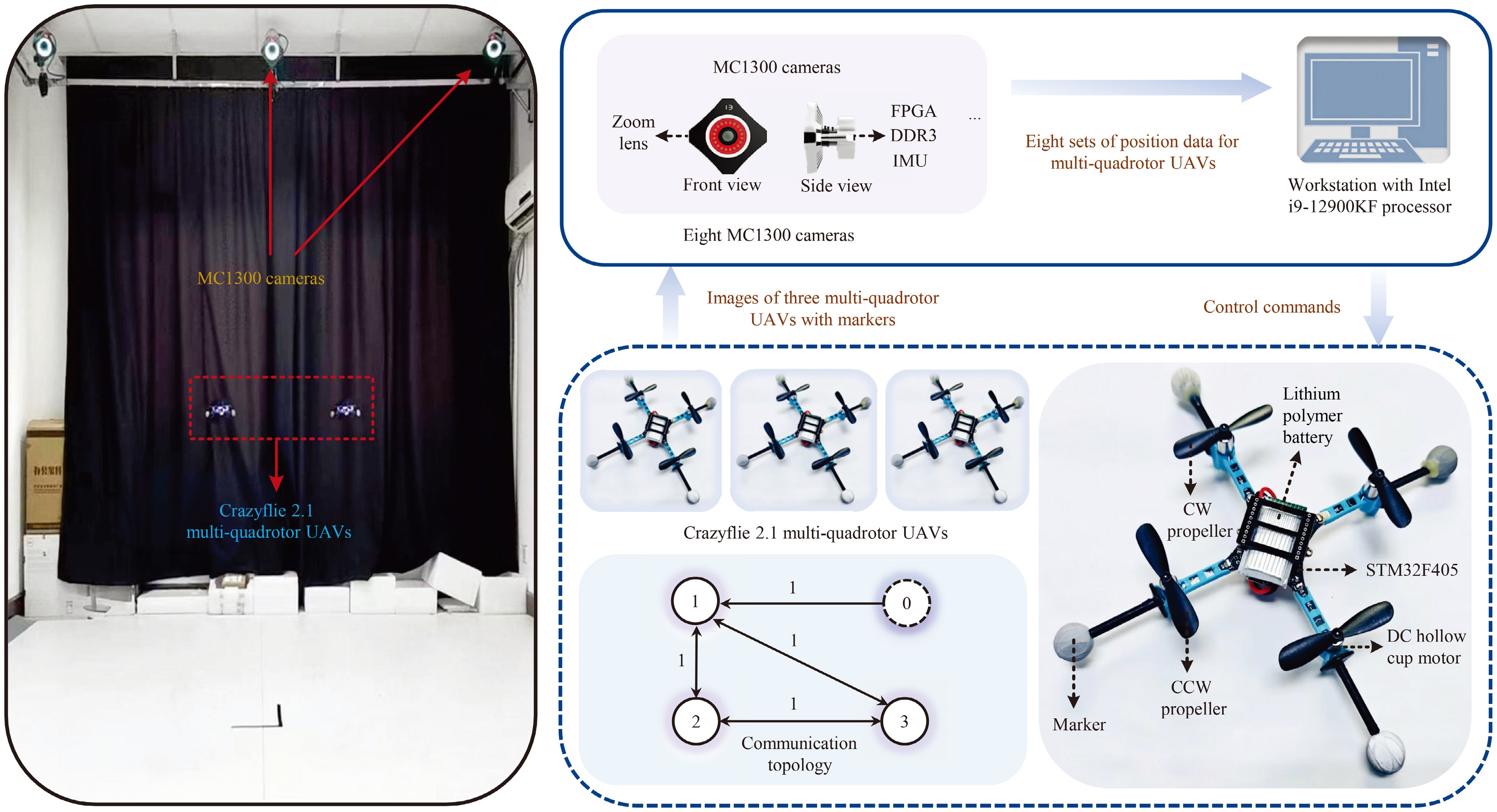
Figure 2.
The experimental platform.
The three multi-quadrotor UAVs are initially positioned at
$ {\boldsymbol{q}}_1(0)=\bigl[0,\,0,\,0.4\bigr]^{T}\,{\rm{m}} $ $ {\boldsymbol{q}}_2(0)=\bigl[0,\,0.2,\,0.4\bigr]^{T}\,{\rm{m}} $ $ {\boldsymbol{q}}_3(0)=\bigl[0,\,-0.2, \,0.4\bigr]^{T}\,{\rm{m}} $ $ \bigl[0,\,0,\,0.4\bigr]^T\,{\rm{m}} $ $ \bigl[2.4,\,1.4,\,0.6\bigr]^T\,{\rm{m}} $ $ n\in\{1,2\} $ $ (x_{c,n},y_{c,n})\in\{(1.00,\,0.45),\ (1.75,\,1.70)\}\,{\rm{m}} $ $ r_{o,n}\in\{0.14,\,0.225\}\,{\rm{m}} $ $ h_{o,n}\in\{0.4,\,1\}\,{\rm{m}} $ $ (x_{c,n},y_{c,n})\in\{(1.00,\,0.45), \ (1.55,\,1.70)\}\,{\rm{m}} $ $ r_{o,n}\in\{0.14,\,0.225\}\,{\rm{m}} $ $ h_{o,n}\in\{0.4,\,1\}\,{\rm{m}} $ $ {\boldsymbol{h}}_1=\bigl[0.10,\,0.00,\,0.00\bigr]^{T}\,{\rm{m}} $ $ {\boldsymbol{h}}_2=\bigl[-0.12,\,0.25,\,0.00\bigr]^{T}\,{\rm{m}} $ $ {\boldsymbol{h}}_3=\bigl[-0.12,\,-0.25,\,0.00\bigr]^{T}\,{\rm{m}} $ $ K_{\text{att}}=0.1 $ $ K_{\text{rep}}^{\text{min}}=0.05 $ $ K_{\text{rep}}^{\text{max}}=0.3 $ $ d_0=0.12\,{\rm{m}} $ $ d_0=0.15\,{\rm{m}} $ $ \mu_1=0.1 $ $ \mu_2=2 $ $ \beta_1=15 $ $ \beta_2=75 $ $ \beta_3=125 $ $ {\boldsymbol{K}}_{pi}={\rm{diag}} \bigl\{4.5,\,4.5,\,5.4\bigr\} $ $ {\boldsymbol{K}}_{di}={\rm{diag}} \bigl\{5,\,5,\,3\bigr\}, i\in{\cal{V}} $ B. Experimental example 1: Results and analysis of cooperative formation obstacle avoidance in sparse obstacle environments.
The experimental results of example 1 are presented in Figs 3a, 4a, 5, and 6. As shown in Figs 3a and 4a, the proposed hierarchical distributed formation obstacle avoidance control scheme enables the three multi-quadrotor UAVs to maintain the desired triangular formation configuration while executing 3D obstacle avoidance maneuvers (overflight and detouring). The responses of the distributed reference signal generator in Eqs (16) and (17) are plotted in Fig. 5, where the second-order virtual followers maintain the desired relative positions with respect to the virtual leader and achieve velocity consensus. Figure 6 depicts the trajectory tracking errors under the composite controller given in Eq. (28). The results show that both the position and velocity tracking errors remain bounded and converge to small residual neighborhoods around the origin, confirming effective tracking of the formation obstacle avoidance references produced by Eqs (16) and (17). Overall, these results validate the effectiveness and feasibility of the proposed scheme in sparse obstacle environments.
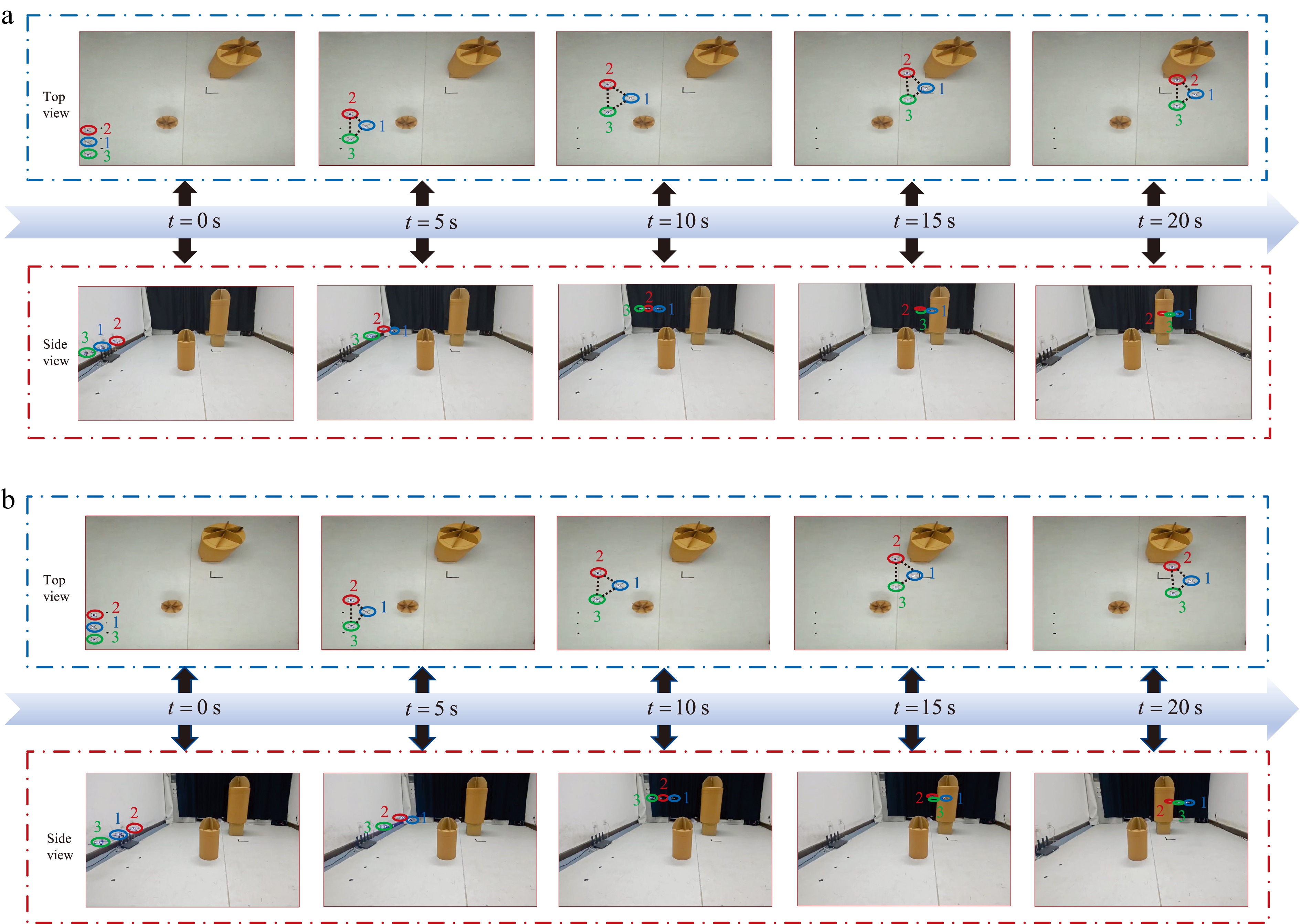
Figure 3.
Experimental images and multi-quadrotor UAV positions at different time instants. (a) Real-time positions of the multi-quadrotor UAVs in example 1. (b) Real-time positions of the multi-quadrotor UAVs in example 2.
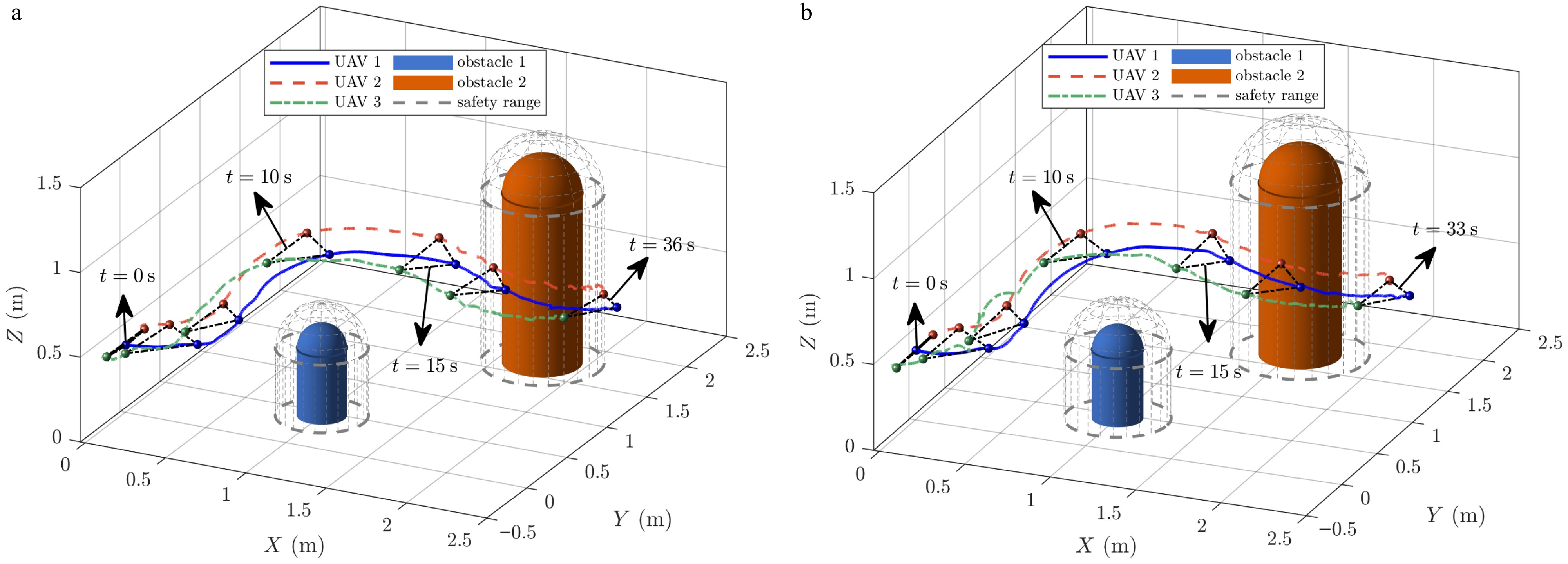
Figure 4.
Trajectories of the multi-quadrotor UAVs in 3D space. (a) 3D trajectories of the formation obstacle avoidance maneuver in example 1. (b) 3D trajectories of the formation obstacle avoidance maneuver in example 2.
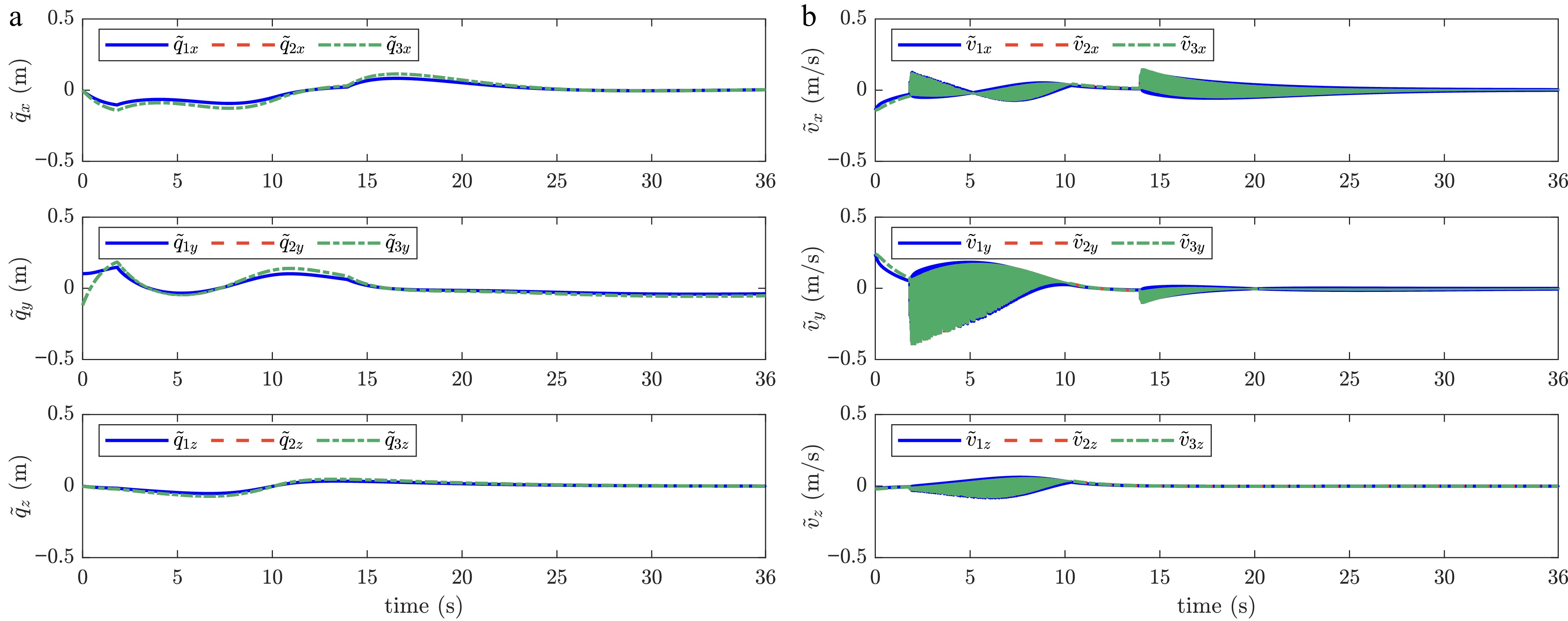
Figure 5.
Response curves of the formation tracking errors under the distributed reference signal generator given by Eqs. (16) and (17) in example 1. (a) Response curves of the formation position errors. (b) Response curves of the formation velocity errors.
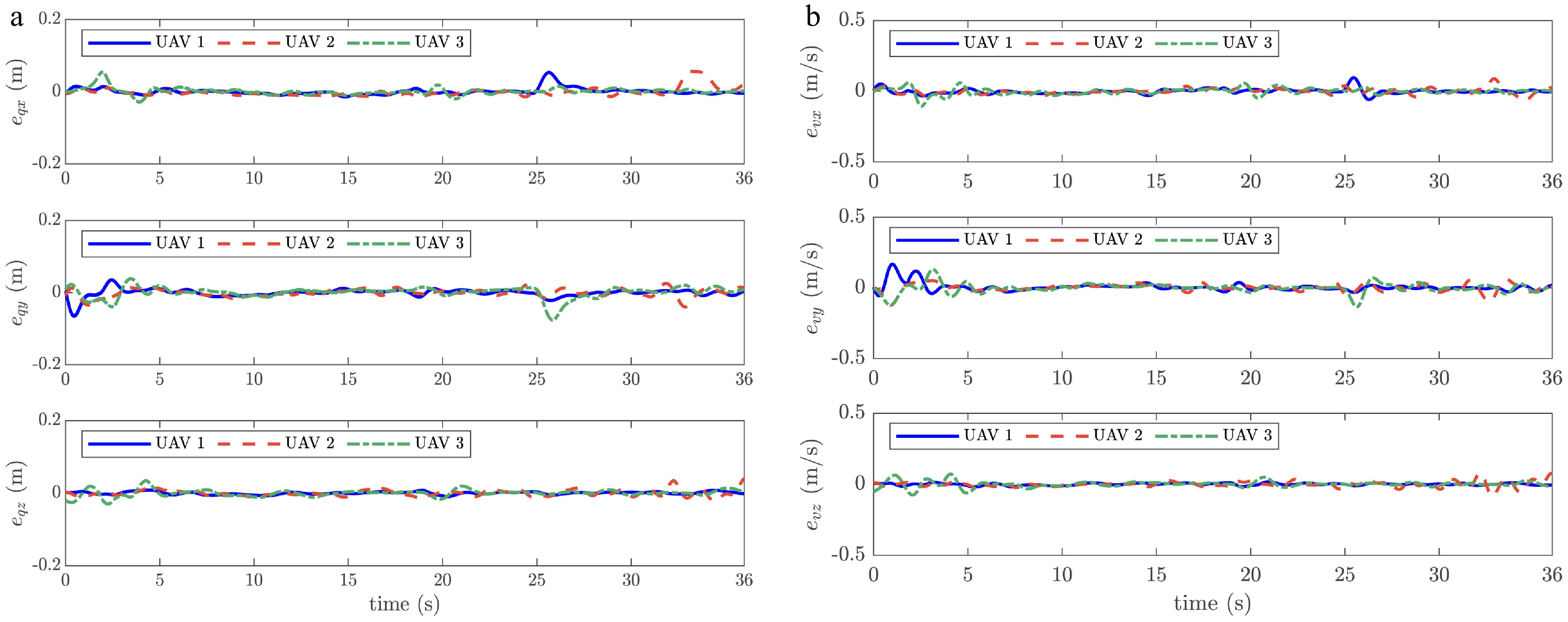
Figure 6.
Response curves of the multi-quadrotor UAVs' trajectory tracking errors under the composite controller given by Eq. (28) in example 1. (a) Response curves of the position tracking errors. (b) Response curves of the velocity tracking errors.
C. Experimental example 2: Results and analysis of cooperative formation obstacle avoidance in dense obstacle environments.
The two obstacles in experimental example 2 are closer than those in experimental example 1. Therefore, a stronger spatial constraint is imposed on the multi-quadrotor UAVs' formation obstacle avoidance trajectory. The experimental results of example 2 are presented in Figs 3b, 4b, 7, and 8. In dense obstacle environments, the proposed hierarchical distributed formation obstacle avoidance control scheme enables the three multi-quadrotor UAVs to perform 3D obstacle avoidance maneuvers (overflight and detouring) while maintaining the desired triangular formation, as illustrated in Figs 3b and 4b. Consequently, the formation configuration is maintained throughout the maneuver, and smooth trajectories are achieved even when obstacles are closely spaced, demonstrating the effectiveness and robustness of the proposed scheme under strong 3D environmental constraints. The response curves of the distributed reference signal generator in Eqs (16) and (17) are presented in Fig. 7, indicating that the second-order virtual followers preserve the desired relative positions with respect to the virtual leader and achieve velocity consensus. The trajectory tracking error responses of the multi-quadrotor UAVs under the composite controller in Eq. (28) are presented in Fig. 8. It is observed that both the position and velocity tracking errors are bounded and converge to small neighborhoods around the origin. Hence, it is verified that the designed composite controller in Eq. (28) achieves robust trajectory tracking in dense obstacle environments. In summary, these experimental results demonstrate the effectiveness and feasibility of the proposed hierarchical distributed formation obstacle avoidance control scheme in both sparse and dense obstacle environments.
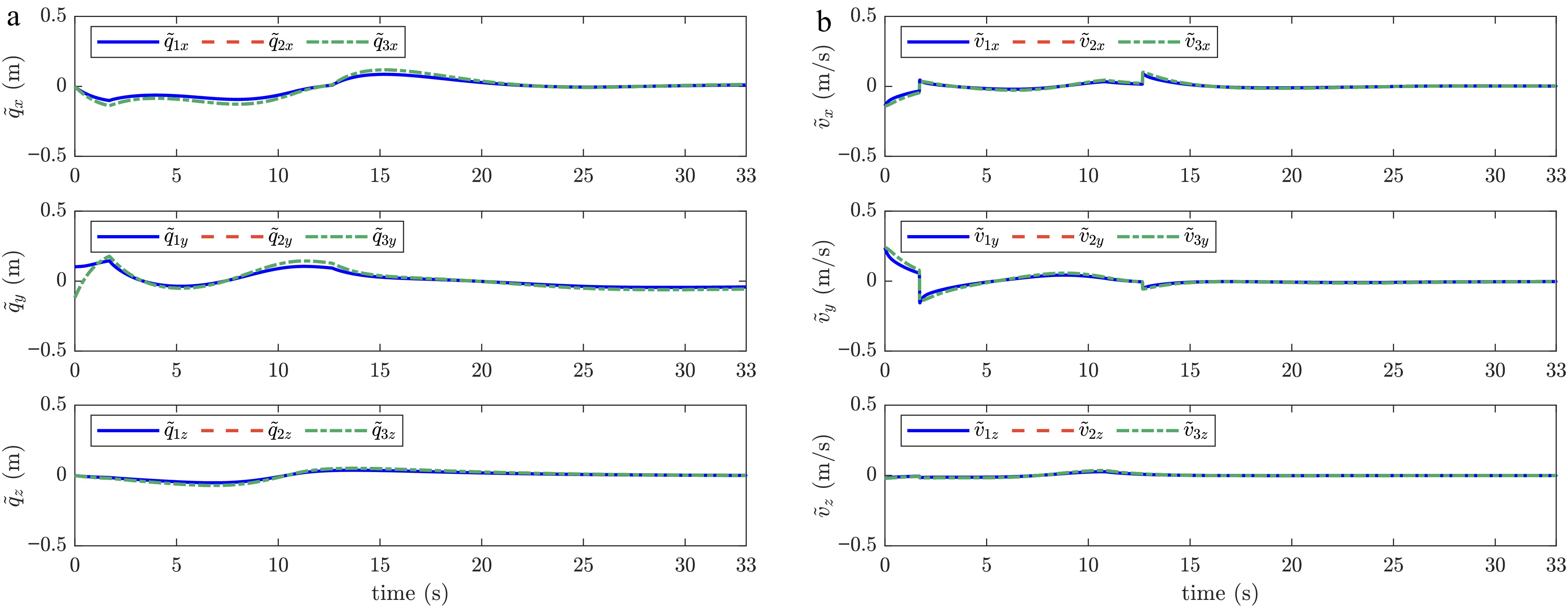
Figure 7.
Response curves of the formation tracking errors under the distributed reference signal generator given by Eqs (16) and (17) in example 2. (a) Response curves of the formation position errors. (b) Response curves of the formation velocity errors.
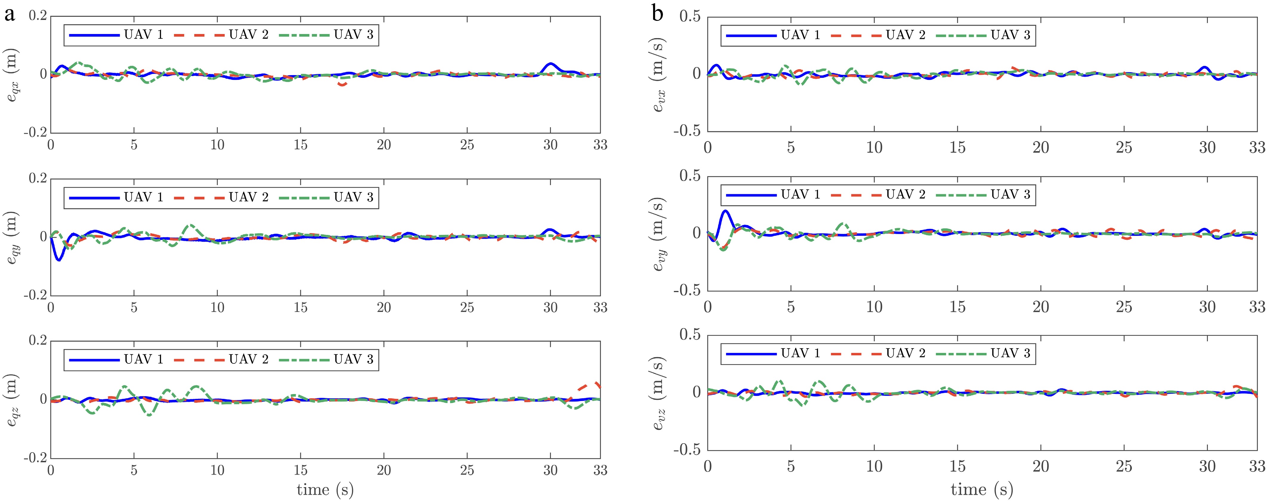
Figure 8.
Response curves of the multi-quadrotor UAVs' trajectory tracking errors under the composite controller given by Eq. (28) in example 2. (a) Response curves of the position tracking errors. (b) Response curves of the velocity tracking errors.
-
In this study, a hierarchical distributed control scheme is developed for multi-quadrotor UAVs that achieves cooperative formation while ensuring 3D obstacle avoidance. An adaptive repulsive gain mechanism is developed within the APF method, mitigating repulsive force jitter near boundaries and reducing the parameter sensitivity inherent in fixed gain designs. The proposed control scheme is composed of two layers, i.e., an upper-layer distributed reference signal generator for formation obstacle avoidance and a lower-layer composite controller for trajectory tracking of the multi-quadrotor UAVs. The two-layer structure improves design flexibility, and the stability analysis demonstrates exponential convergence of the upper-layer formation tracking errors and boundedness of the lower-layer trajectory tracking errors. Experimental results validate the proposed hierarchical distributed formation obstacle avoidance control scheme. Future work will be focused on hierarchical distributed formation obstacle avoidance control for multi-quadrotor systems subject to velocity constraints.
-
The authors confirm their contributions to the paper as follows: study conception and design: Liu Z, Wang X; data collection: Liu Z, Xie F; analysis and interpretation of the results: Liu Z, Wang X, Xie F; draft manuscript preparation: Liu Z. All authors reviewed the results and approved the final version of the manuscript.
-
The datasets generated during and/or analyzed during the current study are available from the corresponding author on reasonable request.
-
This work was supported by the National Natural Science Foundation of China under Grants 62533012 and 62373099.
-
The authors declare that they have no conflict of interest.
- This article is an open access article distributed under Creative Commons Attribution License (CC BY 4.0), visit https://creativecommons.org/licenses/by/4.0/.
-
About this article
Cite this article
Liu Z, Xie F, Wang X. 2026. A cooperative obstacle avoidance control scheme for multi-quadrotor UAV formation: a hierarchical control approach. International Journal of Micro Air Vehicles 18: e005 doi: 10.48130/mav-0026-0004 

A cooperative obstacle avoidance control scheme for multi-quadrotor UAV formation: a hierarchical control approach
- Received: 05 February 2026
- Revised: 13 March 2026
- Accepted: 09 April 2026
- Published online: 22 July 2026
Abstract: In this work, a hierarchical distributed control scheme is proposed to address the cooperative formation and obstacle avoidance problem faced during the application of multi-quadrotor unmanned aerial vehicle (UAV) systems. The distributed control design is decoupled into a two-layer structure consisting of an upper layer for reference signal generation and a lower layer for tracking control. In the upper layer, an adaptive repulsive gain mechanism is introduced into the repulsive force. Based on the adaptive artificial potential field (AAPF) method, an obstacle avoidance trajectory is generated for the virtual leader and it is incorporated into a distributed reference signal generator, which subsequently produces the required reference signals for UAV formation obstacle avoidance. In the lower layer, tracking controllers integrated with an extended state observer (ESO) are designed for multi-quadrotor UAVs. Lyapunov-based stability analysis demonstrates the exponential convergence of the upper-layer error signals and the boundedness of the lower-layer error signals. Finally, the experimental results validate the effectiveness of the proposed control scheme.