dynGBLUP: a unified framework for genomic prediction and association mapping of dynamic phenotypes

As a foundational method in quantitative genetics, best linear unbiased prediction (BLUP) predicts breeding values using a mixed linear model. Its ability to minimize prediction variance while ensuring unbiased estimates has underpinned its widespread application in the genetic dissection of key traits, shortening breeding cycles in animal and plant improvement^[1]. Central to BLUP is the mixed model, a framework that has driven key methodological advances in genome-wide association studies (GWAS) while simultaneously ushering in the era of genomic selection (GS) and genomic prediction (GP) in breeding^[2,3]. As a foundational method within GS, genomic best linear unbiased prediction (GBLUP) estimates marker effects via the genomic relationship matrix, serving as a critical bridge between GWAS and GS. By providing a unified and robust statistical framework for genomic data analysis, GBLUP establishes a solid foundation for genome-enabled selection and stands as a theoretical cornerstone of modern breeding systems^[4,5].

GBLUP translates the principles of quantitative genetics into a practical statistical framework for genomic prediction. Rooted in the infinitesimal model, BLUP assumes an additive genetic architecture in which complex traits are governed by numerous genes of small effect^[4]. This additive assumption provides the theoretical clarity that sets GBLUP apart from current artificial intelligence (AI) approaches, which excel at capturing complex relationships between genotypes and phenotypes but operate as 'black boxes' with opaque internal workings^[6]. For breeders seeking not only predictive accuracy but also mechanistic insight, GBLUP offers a transparent framework in which the influence of relatedness and variance components on random effects can be directly interpreted. In doing so, it transforms genomic prediction from a purely computational exercise into a tool for biological discovery^[7]. GBLUP also aligns with the practical realities of breeding programs: while AI models often require large training datasets and careful hyperparameter tuning to avoid overfitting, GBLUP delivers low overfitting risk, modest computational demands, and statistical robustness in high-dimensional settings^[8−10]. These attributes have secured its central role in contemporary genetic evaluation systems. With the proliferation of AI-based methods, GBLUP has become a widely adopted benchmark for assessing methodological progress. Moreover, the conceptual issues it has raised, such as genotype-by-environment interactions, have actively shaped the development of AI breeding models toward more refined and interpretable directions^[11].

The theoretical value of GBLUP has driven its expansion beyond prediction into broader analytical domains. A key early extension came from Wang et al.^[12], who showed that GBLUP outputs could be transformed into GWAS results by deriving individual SNP effects from genomic estimated breeding values (GEBVs), effectively bridging genomic prediction and association mapping. This translational capacity has since been reinforced by a growing ecosystem of tools, including rrBLUP, ssBLUP, Bayesian models, and BGLR, that support single-trait breeding applications^[13−16], alongside computational packages such as BLUPF90 and DMU that enable industrial-scale genetic evaluation^[17]. Recognizing that complex traits are rarely governed by single or static traits, the field has progressively moved toward multi-trait frameworks. The HIBLUP model, for instance, accommodates multi-trait genomic selection alongside environmental and genetic interactions^[17], while Jung et al. have advanced multi-environment prediction by explicitly modeling genotype-by-environment interactions and envirotyping effects^[18]. The logical next step has been to embrace the temporal dimension of phenotypic expression. Hobby et al. integrated traditional genomic prediction with dynamic mode decomposition (DMD), overcoming the single-time-point limitation of conventional GS to enable dynamic prediction across developmental trajectories^[19]. Collectively, these developments reflect a unifying trajectory: the progressive extension of BLUP models to handle increasingly complex phenotypic data across traits, environments, and time, with the ultimate goal of improving prediction accuracy and biological interpretability throughout entire growth cycles.

The continuous phenotypic variation observed over time represents a critical data source for dissecting the genetic architecture of complex traits. Developing GBLUP models for such data holds the potential to drive transformative advances in GWAS and GS in the era of high-dimensional markers and high-dimensional phenotypes^[20,21]. Unlike single-trait analyses, dynamic traits involve temporal regulation of gene expression. Extending GBLUP to this data type would enable not only genomic prediction across developmental and environmental contexts but also the back-solving of genome-wide SNP effects, thereby integrating prediction with candidate marker discovery in a unified framework^[22,23]. Although research in this area is still nascent, pioneering efforts have established important conceptual foundations. Functional mapping, introduced by Ma and colleagues, first demonstrated the value of fitting growth curves to temporal dynamics or allometric equations to environmental responses, offering breakthrough insights into the genetic basis of development^[24−27]. Subsequent work by Hou et al. advanced this line of inquiry by proposing a nonlinear mixed model that separates random effects from residuals, yet it stopped short of incorporating a genome-wide relationship matrix, thereby limiting its capacity for unbiased estimation of marker effects or breeding values^[28]. More recently, Ning et al. addressed this gap by integrating a genomic relationship matrix into their GMA framework, but they relied on a single non-parametric curve (Legendre orthogonal polynomials, LOPs) to capture phenotypic dynamics, leaving the approach ill-equipped to represent the diverse patterns exhibited by complex dynamic traits^[29]. Collectively, these efforts underscore the need for a GBLUP-based solution that simultaneously models all SNP effects as random effects while accommodating flexible phenotypic trajectories.

To enable dynamic prediction across multiple time points and to facilitate rapid estimation of SNP effects from breeding values, this study integrates the biological principles underlying developmental dynamic gradients. We propose a dynamic GBLUP model (dynGBLUP), designed specifically for dynamic phenotypes. The model accounts for the confounding effects of covariates and relatedness on dynamic phenotypes within a mixed model framework. Building on this foundation, dynGBLUP incorporates growth curves derived from functional mapping theory, including logistic, Gompertz, and Richards^[30−32]. By leveraging the dynamic patterns of phenotypic change over time, dynGBLUP enables systematic dissection of the genetic architecture and dynamic regulatory mechanisms underlying complex high-dimensional traits, thereby advancing breeding decisions from static to dynamic paradigms.

Within the mixed model framework, dynGBLUP is formulated as:

where, y_i represents the vector of phenotypic observations for individual i, measured across multiple time points or environments. W_i, Q_i, and Z_i are design matrices corresponding to fixed effects, SNP random effects, and general random effects, respectively. b is the vector of fixed regression coefficients, u_j denotes the random regression coefficient for SNP_j, p_i represents the coefficients of the general random regression polynomials, and e_i denotes the residual error. The genotype of individual i at SNP_j is indicated by s_ij. The orders of the LOPs are nr₁ for the SNP random effects and nr₂ for the general random effects. In Eq. (1), the second term represents the breeding value obtained by summing the effects of all k genome-wide markers, while the third term accounts for general random effects, such as permanent environmental effects. The choice of LOP order was informed by the work of Ning et al.^[29], who developed a Q + K model for dynamic longitudinal phenotypes. Although that study used LOPs as the only curve fitting approach, their strategy for modeling random effects is directly relevant to ours. Following their successful implementation, we adopted an LOP order of four for random effects. A fourth-order LOP with five parameters provides sufficient flexibility to capture the diversity of random effect trajectories without over-parameterization.

For phenotypic data that follow specific growth patterns, such as logistic or Gompertz functions, these parametric growth curves can be used to model the fixed effects. For phenotypes whose growth trajectories are less well defined, nonparametric LOP curves are employed for fixed-effect modeling. In both cases, LOP curves are also used to model the random effects. The random effects are assumed to follow:

where, $ {{\boldsymbol{\Sigma}}}_{{\boldsymbol{u}}} $ and $ {{\boldsymbol{\Sigma}}}_{{\boldsymbol{p}}} $ denote the variance–covariance matrices of the SNP random regression coefficients and the general random regression coefficients, respectively. The residual variance-covariance structure R is modeled using a first-order structured antedependence model (SAD [1]^[33] with I denotes the identity matrix.

According to Wang et al.^[30], Eq. (1) was linearized using a first-order Taylor expansion, yielding:

where, $ {\tilde{\boldsymbol{y}}}_{i} $ denotes the phenotypic values after transformation, X_i, Q_i, Z_i represent the matrix of first-order partial derivatives of the fixed effects with respect to each parameter of the target growth curve and the two types of random effect function.

Solution of dynGBLUP

Estimation of dynGBLUP relies on the mixed model equations (MME). For Eq. (3), the system is:

The polygenic random effects for individual i, denoted as a_i is considered as the whole of genome-wide marker effect at individual level, is expressed as:

Define C as the coefficient matrix on the left-hand side of Eq. (4), with its inverse given by:

where $ \left(\begin{matrix}\boldsymbol{C}_{22}^{(1)} & \boldsymbol{C}_{22}^{(2)}\\\boldsymbol{C}_{22}^{(3)} & \boldsymbol{C}_{22}^{(4)}\end{matrix}\right) $ = $ \left(\begin{matrix}{\boldsymbol{C}}^{\text{QQ}} & {\boldsymbol{C}}^{\text{QZ}}\\{\boldsymbol{C}}^{\text{ZQ}} & {\boldsymbol{C}}^{\text{ZZ}}\end{matrix}\right) $.

For random regression coefficient for SNP_j, denoted $ {\hat{\boldsymbol{u}}}_{j} $, and its variance are expressed as:

where, $ {\boldsymbol{\Sigma}}_{\boldsymbol{a}} $ denotes the variance–covariance matrix of the polygenic random effects, and K is the marker-derived relationship matrix constructed following the approach proposed by VanRaden^[4]. Based on the solutions for fixed and random effects, with the latter denoting the solved or estimated marker effect, the phenotypic values at the individual level along a temporal sequence can be predicted using Eq. (1). For the statistical significance, the Wald $ {\chi }^{2} $ statistic for each SNP is constructed as follows:

p-values for each SNP are subsequently calculated based on the degrees of freedom (1 + nr₁) to identify significant SNPs. Following Verbyla^[34], all derivations were performed in the framework of the restricted maximum-likelihood (REML). Variance components within the mixed model were estimated, following the iterative algorithm developed by Jensen et al.^[35].

Assessing the type I error rate is critical for evaluating model reliability. For the Q + K model, which accounts for population structure and kinship, realistic simulation of kinship and random effects presents a challenge. To address this, we conducted simulations based on the procedure described in Zhou & Stephens^[36], with the goal of evaluating the model's ability to control false positives under varying sample sizes and heritability levels. Specifically, phenotypes were simulated using real genotype data from the empirical datasets, with quantitative trait loci (QTLs) randomly assigned to explain a proportion of the phenotypic variance. This approach enables a rigorous assessment of the model's type I error rate and statistical power across realistic genetic architectures.

Application to real data

To evaluate the predictive performance of dynGBLUP and its efficacy in QTL detection via back-solved SNP effects, we applied the model to empirical datasets. The dataset was derived from Wei^[37] and consists of a natural population of Populus szechuanica var. tibetica sampled from high- and low-altitude sites in the Sejila Mountains of Tibet, comprising 200 genotypic lines. Populus szechuanica var. tibetica is one of the few tree species that survive on the Qinghai-Tibetan Plateau. Generally, species diversity declines sharply with increasing altitude, and trees rarely occur at very high elevations. The natural distribution of Populus szechuanica under harsh conditions strongly suggests the presence of genetic adaptations that enable survival in such extreme environments. Therefore, our sampling included both high- and low-altitude populations to capture this adaptive genetic variation. Given this design, it is essential to account for potential population stratification in downstream modeling. To prevent this stratification from confounding genetic parameter estimation, we explicitly incorporated the Q matrix as a fixed-effect covariate in the dynGBLUP model^[38]. In 2014, cuttings from this population were propagated in a greenhouse at Beijing Forestry University, and stem diameter was measured throughout the growing season. SNP genotypes were obtained from whole-genome resequencing; after quality control, 24,949 high-quality SNPs were retained. This dataset enables assessment of dynGBLUP's ability to predict dynamic growth traits across multiple time points and to map QTLs underlying temporal trajectories.

To evaluate the predictive performance of dynGBLUP, we compared it with rrBLUP and three machine learning algorithms, i.e., random forest, elastic net, and support vector machine (SVM), following a unified analytical pipeline, including phenotypic dimensionality reduction, coefficient prediction, and curve reconstruction. Specifically, a fourth-order LOP was fitted for each individual according to their growth trajectories. SNPs were then retained as predictors, and separate regression models were trained to predict each coefficient. The predicted dynamic phenotypes were subsequently recovered using the LOP functions. All models were assessed via 10 repeats of 10-fold cross-validation. Pearson correlation coefficient was performed between observed and predicted values.

We evaluated the predictive performance of the dynGBLUP model by performing 10 repetitions of 10-fold cross-validation, using stem diameter data of Populus szechuanica var. tibetica. The model consistently achieved strong predictive accuracy across the dataset. Figure 1a shows the dynamic changes in stem diameter of cuttings from high- and low-altitude populations of Populus szechuanica var. tibetica throughout the growing season. Phenotypic predictions from dynGBLUP yielded an average Pearson correlation of 0.85 between predicted and observed values, outperforming the 0.72 achieved by rrBLUP. We additionally tested three machine learning methods: random forest, elastic net, and SVM, which produced predictive correlations of 0.71, 0.73, and 0.80, respectively. Figure 1b−f further reveals that dynGBLUP better preserved the dynamic characteristics of the Gompertz growth curve, with predicted phenotypic variance across 10 time points ranging from 0.49 to 0.55. In contrast, while rrBLUP captured the overall growth trend, its predictions were largely confined to the mean trajectories of the two subpopulations, with predicted phenotypic variance reaching only 0.04−0.14. The predicted phenotypic variance was 0.027−0.03 for random forest, 0.02−0.03 for elastic net, and 0.28−0.45 for SVM, all of which were lower than that of dynGBLUP and thus failed to capture the full phenotypic diversity of the population.

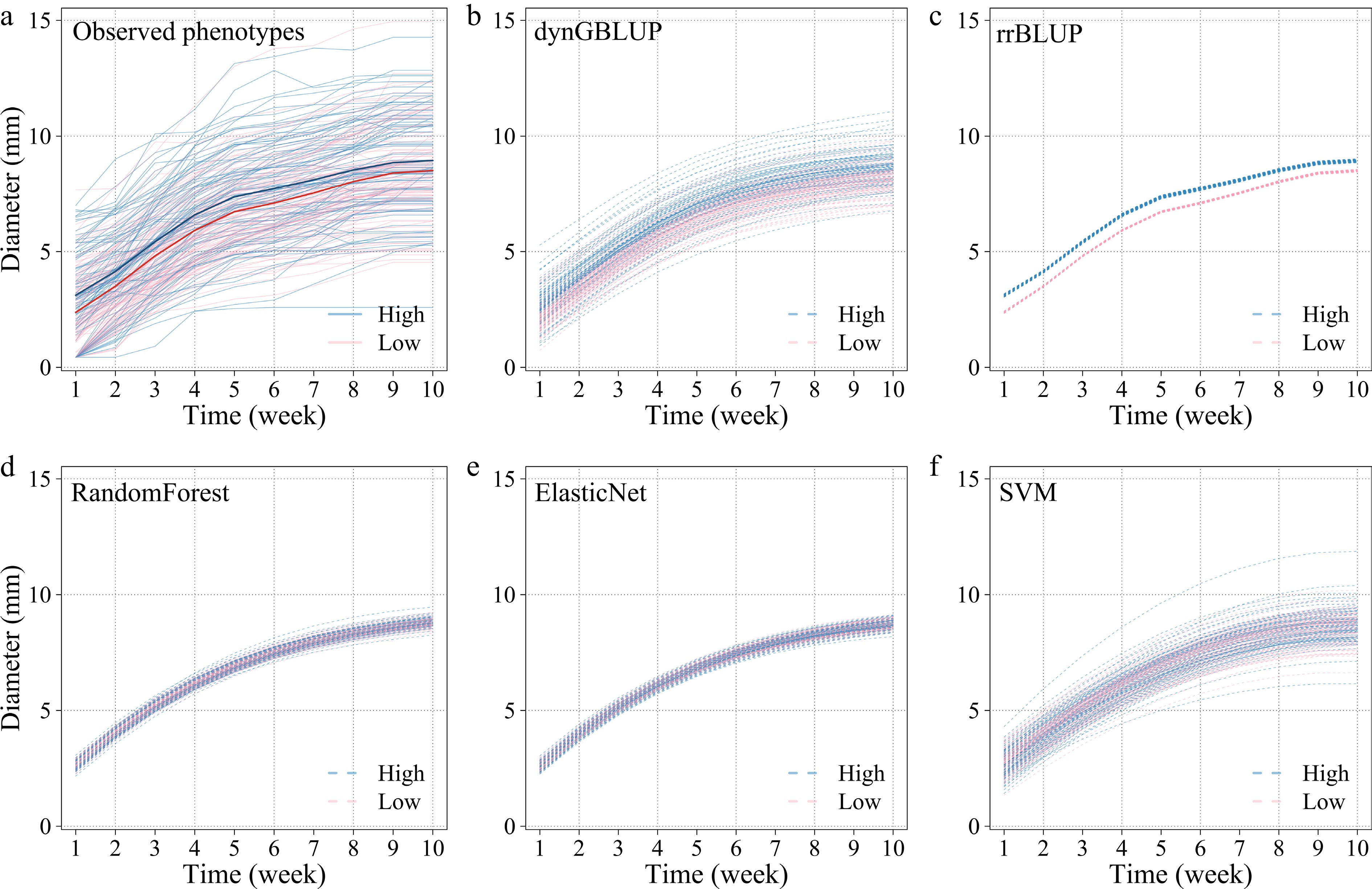
Figure 1. 

(a) Observed stem diameter phenotypes of Populus szechuanica var. tibetica across 10 time points. Average predicted values from 10 repetitions of 10-fold cross-validation using (b) dynGBLUP, (c) rrBLUP, (d) random forest, (e) elastic net, and (f) SVM, for stem diameter data.

To compare model performance in capturing temporal dynamics, we used the Pearson correlation between observed and predicted values as the evaluation metric. Figure 2a shows that dynGBLUP exhibited consistently strong predictive performance across the dataset. For the dynamic growth of Populus szechuanica var. tibetica cuttings, the prediction correlations of dynGBLUP across 10 time points remained around 0.75, with small standard errors ranging from 0.0272 to 0.0308 (Fig. 2a). In contrast, the prediction correlation of SVM was around 0.64, while the correlations achieved by rrBLUP, random forest, and elastic net consistently remained below 0.25. The residual distributions of different models for the stem diameter data of Populus szechuanica var. tibetica are shown in Fig. 2b−f. The residuals of dynGBLUP were approximately randomly and uniformly distributed around zero across the range of predicted values, with small and stable fluctuations and no obvious systematic bias (Fig. 2b). In contrast, the predicted values of rrBLUP were concentrated with small variation, causing the residuals to cluster vertically at a limited number of predicted values and form clear vertical bands, with the residuals tending to increase with higher predicted values (Fig. 2c). The predicted phenotypes of random forest and elastic net were similarly concentrated, and their residual plots also exhibited distinct vertical banding at early growth stages (Fig. 2d, e), indicating that these three models likewise failed to adequately capture the true phenotypic variation in the population. The residuals of SVM showed a relatively random distribution, similar to that of dynGBLUP (Fig. 2f).

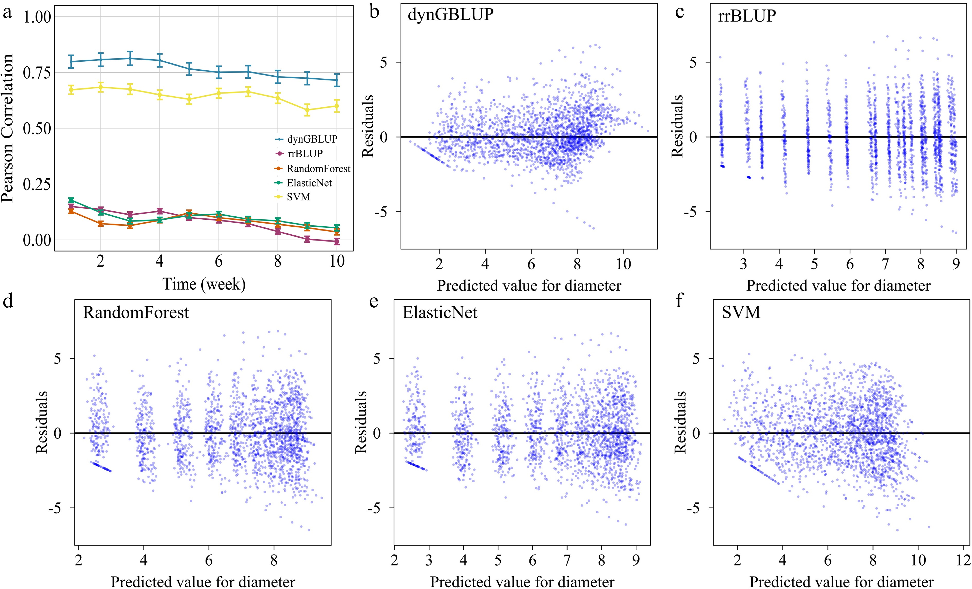
Figure 2. 

(a) Comparison of the predictive performance of dynGBLUP and rrBLUP models across individual time points. Predicted residuals from (b) dynGBLUP, (c) rrBLUP, (d) random forest, (e) elastic net, and (f) SVM, for stem diameter growth in Populus szechuanica var. tibetica cuttings.

By estimating genome-wide marker effects and providing a framework for evaluating SNP significance via Eq. (9), dynGBLUP inherently supports GWAS. To evaluate its performance, we employed a simulation strategy in which the phenotype-genotype correspondence was randomly shuffled to reconstruct phenotypic datasets. Figure 3a shows that when heritability was set to zero, the type I error rate was controlled between 9.40% and 16.91%. Figure 3b indicates that detection power strongly depends on heritability, increasing substantially as heritability rises. When the sample size exceeded 800, the gain in power from additional samples was smaller than the increase attributable to higher heritability. Under a sample size of 1,000 and a heritability of 3%, the model achieved a detection power of 77%. These results demonstrate that dynGBLUP provides high power for GWAS when applied to multi-time phenotypic data.

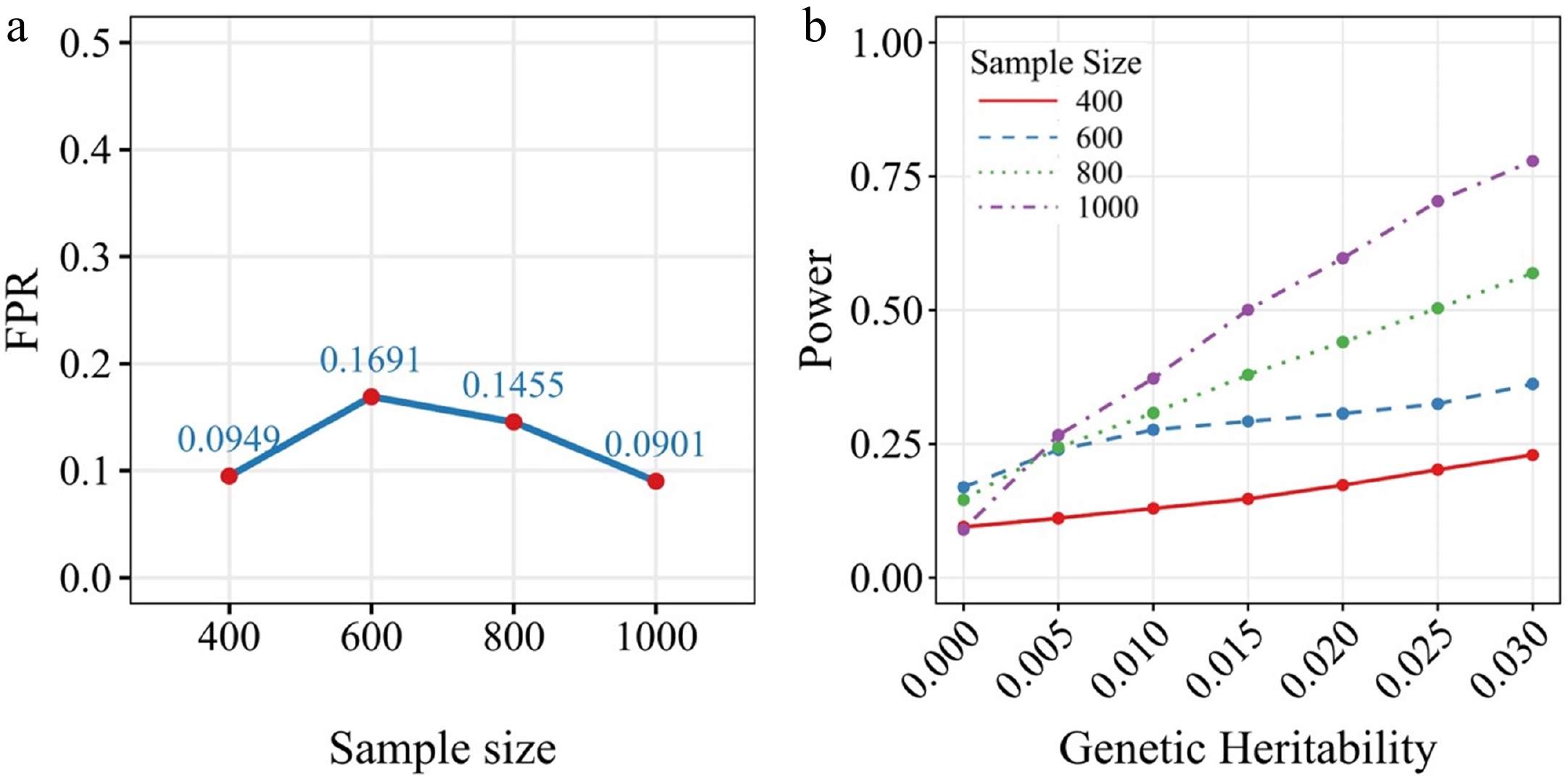
Figure 3. 

(a) False positive rate and (b) statistical power of the dynGBLUP model.

To further evaluate the GWAS utility of dynGBLUP, we computed SNP p-values from the genetic effects estimated by the model using empirical data. The stem diameter dataset yielded robust association mapping results. The Manhattan plot showed that significant SNPs were widely distributed across the genome (Fig. 4a). Based on functional annotation, THESEUS1 encodes a brassinosteroid-regulated receptor kinase known to regulate overall plant growth by mediating cell elongation during the vegetative growth stage; LOC7490611 with its homology of At5g40410 in Arabidopsis is highly expressed during young leaf growth, suggesting it may play a positive regulatory role in leaf development and overall plant growth; SRG1 responds to intracellular sugar content at the transcriptional level^[39]. Because sugar signaling plays a central role in regulating plant growth, energy metabolism, and senescence, this gene may influence overall plant growth by mediating sugar homeostasis. The QQ plot indicated that 99.4% of SNPs conformed to the expected distribution, with upward deviation observed only in the extreme tail corresponding to a p-value threshold of 0.0038 (Fig. 4b). Collectively, these results demonstrate that estimating SNP effects within the dynGBLUP framework provides a unified approach for simultaneous GWAS of dynamic traits.

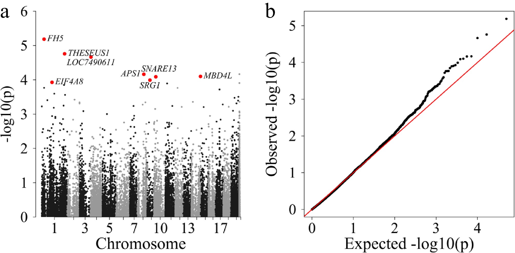
Figure 4. 

(a) Manhattan and (b) QQ plots for stem diameter growth in Populus szechuanica var. tibetica cuttings.

As a core method in genomic selection and prediction, GBLUP has driven a paradigm shift in modern breeding, transitioning from posterior-based phenotypic selection to prior-based genomic prediction^[40,41]. This transition has overcome key limitations in leveraging molecular marker data to estimate GEBVs, enabling breeding decisions to be made at early stages with greater precision and efficiency. With the rise of intelligent breeding, there is growing recognition that developmental stages critically influence key phenotypic traits in both plants and animals, spurring the development of dynamic genomic prediction^[42,43]. To address this challenge, we propose the dynGBLUP model, which predicts dynamic phenotypes at specific developmental stages while simultaneously estimating genome-wide marker effects. This framework offers a novel strategy for predicting dynamic traits across multiple time points using genome-wide markers, enabling breeders to select for target traits while optimizing growth trajectories encoded in the underlying genetic architecture.

By integrating time-series, dynGBLUP incorporates the developmental dynamics of biological traits through a range of growth curves. Capturing the dynamic genetic regulatory mechanisms underlying growth and development, this framework enables prediction of phenotypes at specific developmental stages. Simultaneously, its statistical structure allows estimation of genetic effects for individual SNPs within a 'one-step GWAS' framework. When estimating SNP effects, researchers often encounter the 'curse of dimensionality', in which the number of SNPs (p) greatly exceeds the sample size (n). To mitigate the risks of overfitting and overparameterization arising from a rank-deficient design matrix in least-squares methods, dynGBLUP employs the BLUP estimation approach. In Eq. (1), the random effects component encompasses genome-wide SNPs. When translating the output into GWAS results, if we define the polygenic effect as the sum of individual marker effects, it can be equivalently expressed in a form that satisfies the Q + K model commonly used in GWAS. Taken together, dynGBLUP provides a robust bridge between GS and GWAS for traits exhibiting temporal dynamics, highlighting the consistency of statistical frameworks for analyzing dynamic phenotypes within both GBLUP and GWAS.

Given the critical role of dynamic traits in elucidating the genetic architecture of complex biological traits, Ning et al. developed a GMA-based association analysis algorithm for multi-time-point phenotypes^[29]. However, their approach relies solely on non-parametric LOP curves, limiting its ability to accurately capture diverse biological growth patterns and developmental trajectories. In contrast, the present study builds upon the theoretical framework of functional mapping and integrates multiple types of growth curves to systematically characterize dynamic and quasi-dynamic patterns of phenotypic variation over time or along environmental gradients. We developed a GBLUP framework tailored for dynamic phenotypes by employing SAD(1) to model the variance–covariance structure of dynamic phenotypic residuals. The successful use of Gompertz equations enables more biologically meaningful fits for fixed effects and more accurately reflects the principles of development. This approach overcomes the limitations of traditional non-parametric basis functions in capturing complex developmental traits, thereby enhancing analytical flexibility for intricate dynamic phenotypes. The assumption of a shared baseline growth curve is indeed a common and biologically starting point for many dynamic models. For a given trait, the underlying growth pattern (e.g., a logistic or Gompertz curve) is generally similar across individuals, which is consistent with basic biological principles. Individual differences manifest as deviations from this common baseline, and our model explicitly captures such heterogeneity through multiple components: (1) random regression coefficients that allow individual-specific curve adjustments; (2) the Q matrix (population structure) as fixed effects, which accounts for systematic differences between subpopulations; and (3) heterogeneous residual variances. This modeling strategy is conceptually analogous to how a standard regression framework handles the overall mean $\mu $, a shared baseline (akin to $\mu $) plus systematic differences captured by fixed effects (such as the Q matrix for population stratification) and additional individual-specific random deviations. Therefore, we believe the assumption is reasonable and sufficiently flexible for the data at hand. The dynGBLUP model was validated using the real dataset and computer simulations, with comparisons to rrBLUP and multiple machine learning methods. It consistently achieved high Pearson correlation coefficients in genomic phenotype prediction across multiple time points, demonstrating both feasibility and accuracy for complex dynamic traits.

Notably, Hobby et al. combined DMD with genomic prediction to construct the dynamicGP model, which is capable of predicting the dynamic growth of multiple traits^[19]. However, dynamicGP relies on the preprocessing of high-dimensional time-series phenotypic data, and its performance depends on the number of input traits and time points, making it best suited for physiologically related traits. In contrast, dynGBLUP directly targets key agronomic traits, such as plant height and stem diameter, without relying on dynamic mathematical decomposition or additional traits, serving as a complementary rather than competitive approach to existing genomic prediction algorithms. A key assumption underlying dynGBLUP is that SNP effects follow a homoscedastic random-effects distribution, consistent with the infinitesimal model in which each SNP contributes a small effect. While this assumption provides a computationally tractable and interpretable framework, future extensions could incorporate Bayesian sparse models to enhance the accuracy of effect estimation for loci with larger phenotypic contributions. For multi-environment phenotypic data, the current use of population means as environmental indices could be refined by integrating more biologically meaningful environmental covariates, as exemplified by recent advances in envirotyping^[44]. Collectively, these extensions point toward a broader vision: transitioning genomic selection from predicting static, singular genetic potential toward a framework that embraces dynamic, plastic, and stable selection.