Agronomic performance, genotype x environment interaction, and stability of leaf yield of Jute mallow (Corchorus olitorius L.) in Burkina Faso

Opportunity crops, such as indigenous African leafy vegetables, have been incorporated into human diets, especially in sub-Saharan Africa and many Asian countries, where they greatly contribute to food and nutritional security^[1,2]. These indigenous African crops have high agronomic and nutritional potential that could contribute to improving food and nutritional security. They can be used to fight 'hidden hunger'^[3−5]. Corchorus olitorius (L.) is one of the indigenous African crops. It is found in the wild, but is increasingly cultivated in many tropical countries in Africa^[5−7]. Fresh and dried leaves of C. olitorius produce a sticky sauce like okra; when dried, they can be stored whole or in powder form^[8]. Its edible parts are rich in vitamins (A, C, and D), essential nutrients (β-carotene, amino acids, carbohydrates), and minerals (potassium, calcium, iron, zinc)^[9−11]. According to some authors^[12−15], due to its phytochemical and antioxidant properties, jute mallow can be used to solve nutritional deficiencies.

In Burkina Faso, jute mallow is of high socioeconomic importance for value chain participants. It is cultivated and consumed in urban and peri-urban farming systems^[16,17]. The fresh, dried, and cooked leaves are a common accompaniment to many local dishes based on cereals (such as rice, corn, and sorghum), tubers (such as yams), and/or roots (cassava). Despite its socioeconomic importance to the local population, the lack of productive varieties is a major obstacle to realizing this plant's agronomic and nutritional potential. Indeed, agromorphological, molecular, and biochemical characterizations have identified genotypes with high agronomic and nutritional potential^[10,15−17]. However, the agromorphological characterizations were conducted at a single site. Consequently, these trials did not identify genotypes with high and stable agronomic performance. Selecting high-yielding and stable varieties through trials in a single environment is ineffective^[18,19]. In fact, factors such as temperature, precipitation, and the physicochemical composition of the soil influence plant growth and productivity. It is necessary to account for these factors in breeding and variety improvement programs^[20]. In other words, the performance of genotypes results from the genotypic effect (G) of the genotype, the environmental (E) effect in which the genotype is grown, and the interaction between genotypic and environmental effects (GEI)^[21−23]. Consequently, an assessment of landraces in contrasting sites enables the selection of genotypes adapted to specific environments. Indeed, in crop breeding programs, the identification of high-performing and stable varieties presents a major advantage for plant breeders. This study aims to (i) evaluate the agronomic performance and (ii) to identify high-yield and stable genotypes of a collection of jute mallow in Burkina Faso.

The plant material included eighteen genotypes from the gene bank of the Plant Genetics and Breeding Team of the University Joseph KI-ZERBO and two varieties from the World Vegetable Centre (Table 1; Fig. 1). The genotypes were selected based on their agronomic performance from previous evaluations^[10,16,17] and communities' preferences. The two varieties from WorldVeg, used as checks in this study, are currently being released in Burkina Faso.

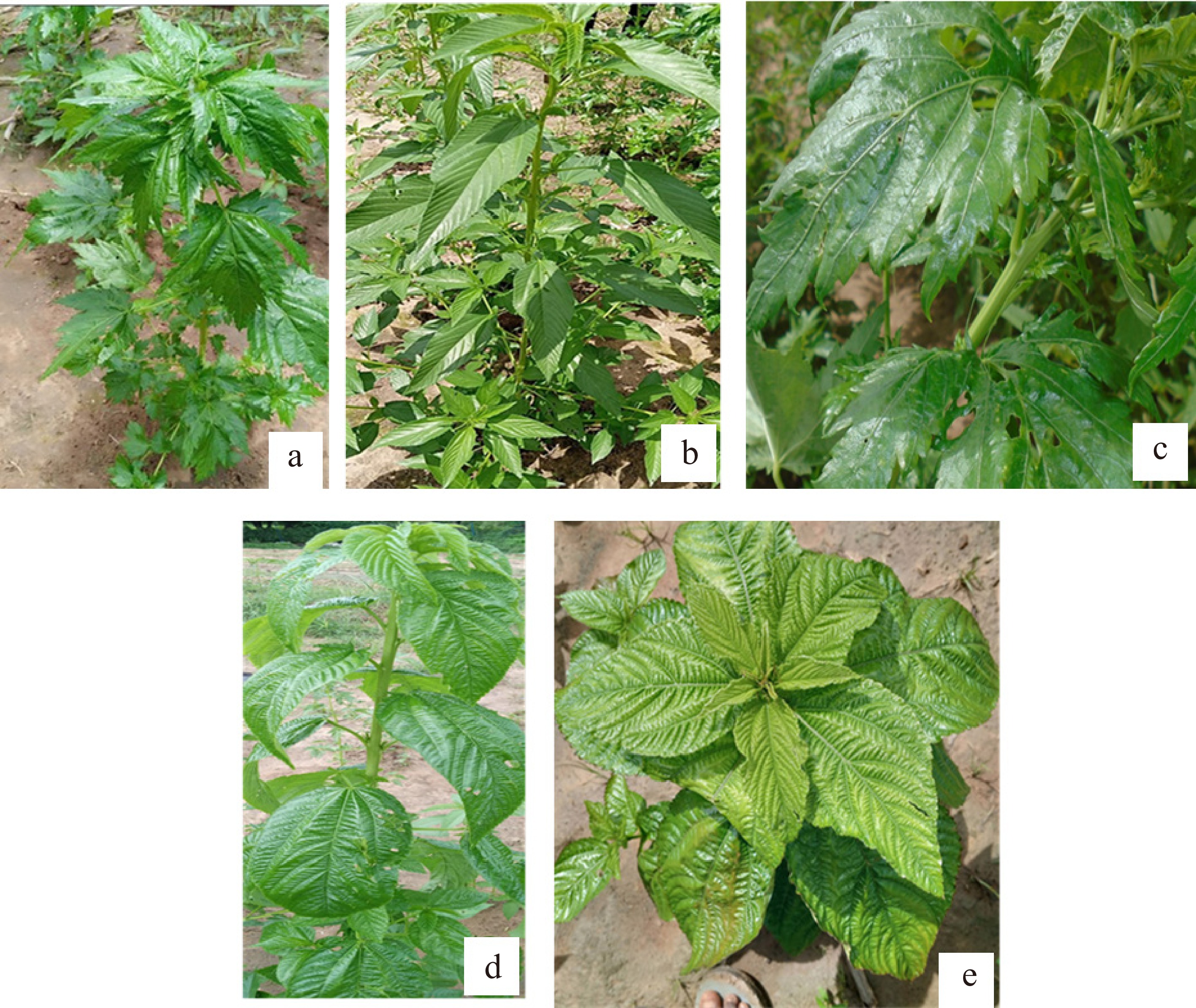
Figure 1. 

Characteristics of some genotypes and two varieties used in this study.

(a) SBL1; (b) KOL; (c) HBV9; (d) BIG; (e) AZIGA; (a, b, and c) genotypes from Burkina Faso, (d and e) varieties from WorldVeg.

Description of the study sites

The agronomic trials were conducted in three peri-urban zones, Bourbo (E1), Gampela (E2), and Sogossagasso (E3), located in the three agroclimatic zones of Burkina Faso, respectively. Bourbo (latitude 13°34′ N and longitude 2°25 E) is located in the Sahelian climatic zone, Gampela (latitude 12°15′ N and longitude 1°12′ E) in the Sudano-Sahelian zone, and Sogossagasso (latitude 11°38′ N and longitude 4°07′ E) in the Sudanian climatic zone. The three agroclimatic zones are characterized by an annual rainfall gradient that increases from north to south. Thus, during the experiment, the three locations received cumulative rainfall of 625.8, 771.8, and 832.4 mm, respectively (Table 2). At Bourbo, the soil exhibited a sandy-silty texture with 82.35% sand, 15.69% silt, and 1.96% clay. Regarding Gampela, the soil texture class was also sandy-silty, with 82.35% sand, 13.73% silt, and 3.92% clay. At Sogossagasso, the soil texture class was sandy, with 90.20% sand, 7.84% silt, and 1.96% clay. In these three sites (Burbo, Gampela, and Sogossagasso), the pH was slightly acidic, 5.70, 5.95, and 5.92, respectively.

Experimental design and conditions of cultivation

The agronomic trials were conducted from July to October 2022 under rainy conditions. The planting took place on July 05, 10, and 15, 2022, respectively, in Sogossagasso, Gampela, and Bourbo, corresponding to three different environments (E1, E2, and E3). The genotypes were evaluated across the three environments using randomized complete block designs with three replications. First, seeds of the genotypes were used to set up a nursery. Then, the resulting seedlings were transplanted to the experimental plot 3 weeks later. Each replicate measured 9.4 × 6 m, and the distances between blocks were 1.5 m. The genotypes were randomly distributed to the rows. Every experimental unit consisted of one row of 6 m with 0.5 cm spacing between rows and 0.5 cm spacing between plants, resulting in 13 plants per row. Four weedings were done manually in each location.

Data collection

Table 3 shows the quantitative data that were collected. Except for the number of days to 50% flowering determined per row, the other characters were measured on five randomly selected plants per row.

Data analysis

The agronomic data were conducted using R (4.5.1). A two-way analysis of variance (genotypes G, environments E, and G x E interaction) was realized using the metan package to determine significant differences between genotypes and locations in evaluating the level of G x E interaction. Before the analysis of variance, the Shapiro–Wilk test was used to assess the normality of the data. Subsequently, Bartlett's test of homogeneity of variances was performed to verify the homogeneity of variances of the measured variables across environments. The classification of the locations was based on the ANNICCHI-ARICO^[24] method through the estimation of the environmental index. Based on this index, the locations were classified as favorable or unfavorable. Heat maps illustrating the mean yield of the genotypes across three locations were generated with the 'tidyverse' and 'ggplot2' packages. Additionally, a GGE biplot analysis was performed in combination with ggplot2 for graphical visualization to identify the ideal genotype (high-yielding and stable genotype) and the ideal environment. Thus, based on genotype plus genotype by environment (GGE) biplot analysis methods^[25−27], graphs showing: (i) the classification of genotypes according to mean yield and stability; and (ii) an assessment of the test environments were generated. In addition, stability parameters (Table 4) were estimated using parametric and nonparametric analyses. The formulas used to calculate these stability parameters are those reported in studies by Herawati et al., Kyratzis et al., and Fiseha et al.^[28−30].

The results of the preliminary analyses (Table 5) indicate that the variances of all the variables studied are homogeneous. Significant differences between genotypes for all agronomic variables were highlighted (Table 6). In addition, highly significant GEN × ENV interactions were exhibited for the five quantitative traits. Highly significant effects of environment (location) were observed for days to 50% flowering, plant height, stem diameter, number of branches per plant, and leaf yield. The coefficient of variation ranged from 9.77% for days to 50% flowering to 81.89% for leaf yield. A comparative analysis of the average performance of the genotypes studied (Table 7) shows that plant heights range from 78.708 to 134.556 cm for genotypes AZIGA and HBV9, respectively. Regarding 50% flowering and plant height, genotype AZIGA flowered late (69.250). Based on plant height (134.556 cm), stem diameter (15.181 mm), and number of branches per plant (21.741), HBV9 exhibited the best performance. Coming to leaf yield, genotype SKY1, with a mean value of 9,712 t/ha, showed good performance. However, the lowest yield (3,236 t/ha) was observed for genotype GIT.

Analysis compares the mean performance of genotypes for leaf yield (t/ha) across locations

The highest yield was observed at E2 for genotype SKY1 (average of 19.236 t/ha), and the lowest yield was obtained at E1 for KAB2 (1.231 t/ha). Except for genotypes GTI, AZIGA, and BIG, which obtained better leaf yield at site E3, the other genotypes showed better leaf yield in site E2. Table 8 indicates the mean leaf yield of genotypes across the environments.

Stability of yield

Graphical illustration of the mean yield performance of genotypes using the tidyverse and ggplot2 packages

The results of the analysis (Fig. 2) highlight genotypes with superior performance in yellow, while genotypes with low leaf yield are shown in black or blue-black in the different environments. Considering the genotype, the leaf yield, with a mean of 6.1 t/ha, varied from 3.2 for GIT to 9.7 t/ha for SKY1. For an overall yield of 8.3 t/ha, SBL1 obtained 8.1, 11.7, and 5.3 t/ha for E1, E2, and E3, respectively. The overall mean across the three environments for the 20 genotypes ranged from 3.038 to 10.875 t/ha at E1 and E2, respectively. Moreover, with environmental index values of −3.11 and −1.62, respectively, for E1 and E3, these two environments are unfavorable compared to E2, whose environmental index was 4.73 (Table 9).

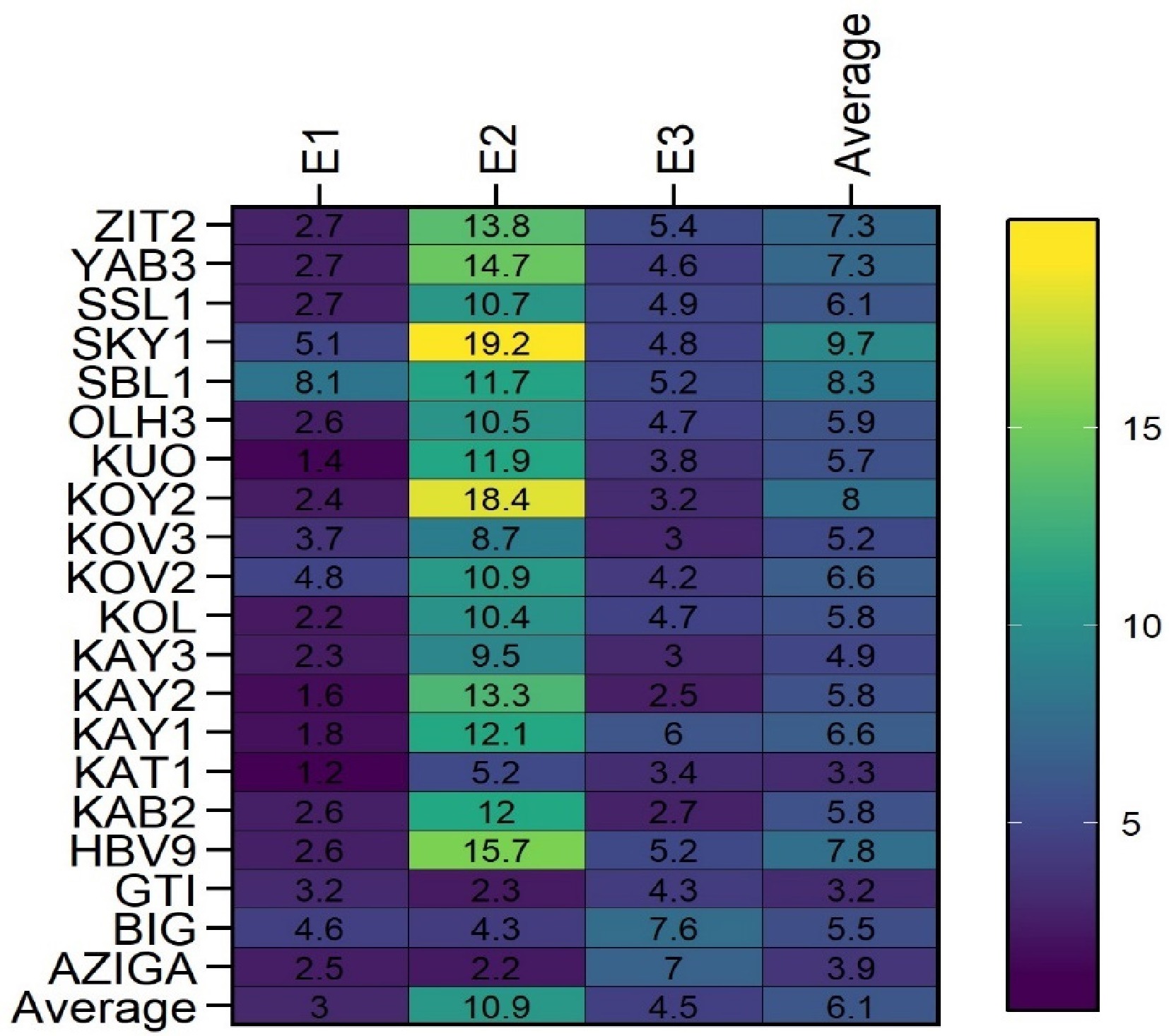
Figure 2. 

Heat map illustrating the average yield of genotypes across three locations to visually assess G × E interactions: Ouahigouya (E1), Gampela (E2), and Sogossagasso (E3).

Genotype yield and stability performance

The result of the biplot 'mean vs stability' (Fig. 3) indicates that when the projection of a genotype with respect to the PC1 axis (abscissa axis) is high, the lower its stability. Conversely, the further a genotype is located from the PC2 axis (ordinate axis), the more yielding it tends to be. The arrow indicates the highest average performance among the evaluated genotypes. The first two principal components explained up to 94.83% of the total variation among genotypes. Thus, the genotypes located close to the arrow obtained the highest leaf yield (RL). The mean stability biplot demonstrated that genotypes SKY1 and SBL1 exhibited high leaf yield (LY). In contrast, genotypes GTI, KAT1, and AZIGA exhibited the lowest leaf yield (LY). Stable genotypes were identified by observing the vector length (dotted line) between the average environment axis and the location of each genotype. Thus, KOV2 and SBL1 were identified as the most stable genotypes, while AZIGA, BIG, and KOY2 were the least stable. Genotype SKY1 performed better than the other genotypes. However, it is less stable than KOV2 and SBL1.

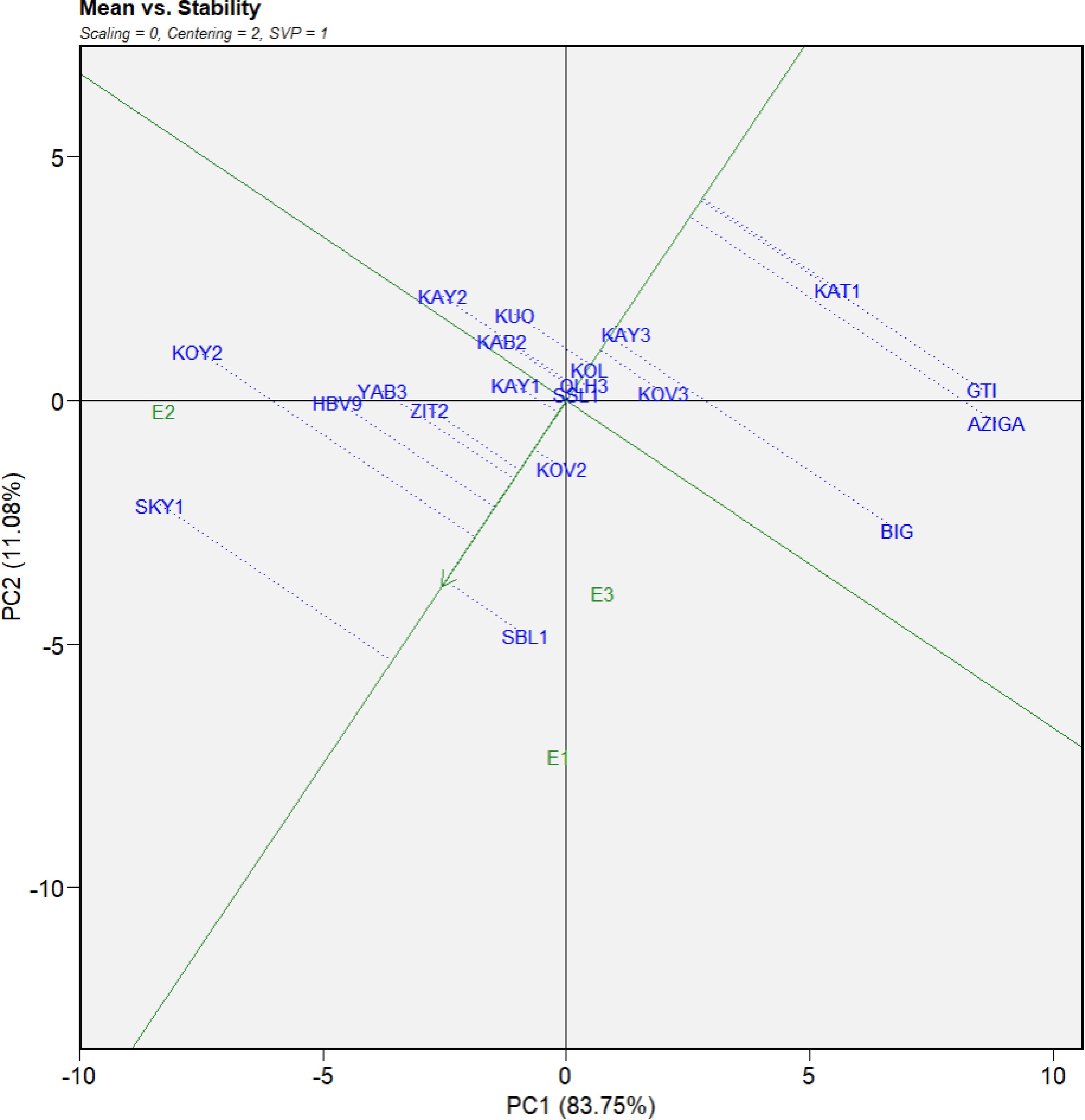
Figure 3. 

The ranking biplot shows the mean performance and stability of 20 Jute mallow (C. olitorius) genotypes across three locations: Ouahigouya (E1), Gampela (E2), Sogossagasso (E3).

Ranking and identification of ideal genotypes

The GGE biplot (Fig. 4) ranks the genotypes, with the ideal genotype located at the epicenter of the concentric circles. According to this representation, the genotypes that are plotted close to the epicenter are close to the ideal genotype in terms of yield production and stability averaged across environments. Thus, the ranking of genotypes close to the ideal genotype at the epicenter was SBL1 > KOV2 > ZIT2 > HBV9 > YAB3 > SKY1 > KAY1. The genotype SBL1 (8.3 t/ha), ranked second in terms of leaf yield is the most stable genotype, the SKY1 genotype (9.7 t/ha) which presented the best leaf yield is ranked sixth for stability.

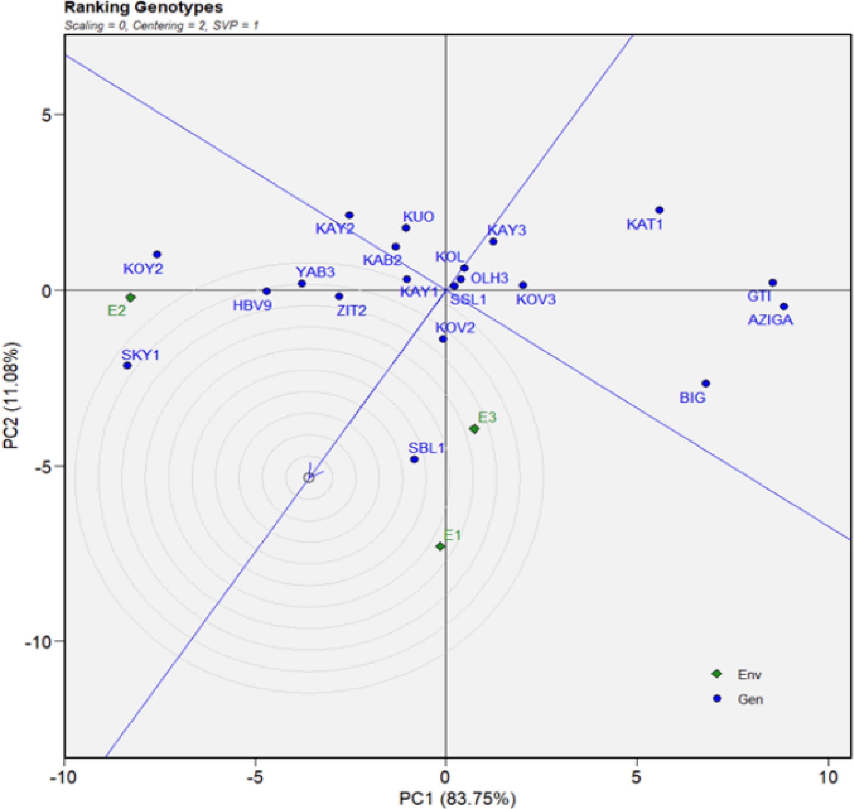
Figure 4. 

GGE-biplot showing the ideal genotypes. Ouahigouya (E1), Gampela (E2), Sogossagasso (E3), genotype (Gen), and environment (Env).

Estimation of stability using parametric and nonparametric statistics

The results of the stability parameters, calculated using parametric and nonparametric statistics, and the average yields of the 20 genotypes are presented in Table 10. Specifically, the AZIGA, BIG, and GTI genotypes, with a regression coefficient significantly lower than unity (bi < 1), are adapted to unfavorable environments. In contrast, the genotypes KOY2 (bi = 2.08) and SKY1 (bi = 1.89), with a regression coefficient significantly higher than unity, are adapted to favorable environments. As for the regression residual (S²di), it is not significant for any of the genotypes. Consequently, the BIG and AZIGA genotypes, with S²di > 0 and below-average yield, are highly unstable. The YAB3, HBV9, ZIT2, KOV2, KOY2, and KAY1 genotypes, which have average yields above the overall average and S²di < 0, are stable. The ranking of the five most stable genotypes, based on the other stability parameters, is presented in Table 11. According to this ranking, with the exception of Wi and Pi, the OLH3 genotype, with a yield of 5.94 t/ha, ranks among the top five most stable genotypes. For the Wi and Pi values, SKY1 (9.71 t/ha) ranks first in terms of stability, fifth for S3, and fourth for S6, respectively.

The study exhibited a variation in the agronomic performance of genotypes depending on location and a significant genotype–environment interaction. This indicates phenotypic diversity among the genotypes and that they respond differently to environments. Moreover, the variation in genotype performance across environments suggests the possibility of selecting genotypes adapted to each specific environment. The highly significant genotype effect (< 0.001) across all variables confirms a very large phenotypic variability, which offers opportunities for selection and varietal development. Moreover, the shift in mean performance of some genotypes from the mean suggests that these genotypes are potential sources of favorable genes that may be useful for the breeding programs of jute mallow. Thus, HBV9, which has the highest number of branches, the tallest and the thickest stem, can be considered as a genotype with characteristics sought after in plant breeding. Indeed, in leafy vegetable breeding, plant vigor, plant height, number of branches, and latest flowering are key selection criteria for the leaf yield improvement^[39,40]. Therefore, the low yield of AZIGA would be linked to its small size and few branches, although it has the longest flowering cycle.

Elsewhere, the highly significant effect (p < 0.001) of environmental variation and the significant mean squares of the environments for all the studied variables indicate that the varieties must be released according to their adaptability. In fact, although agronomic performance depends on genotype, it is also strongly influenced by pedoclimatic factors, such as temperature, precipitation, and soil physiochemistry^[41,42]. Thus, the low yield of accessions observed in E1 and E3 would be linked to their agroecological conditions. Therefore, for a better expression of the production potential of the genotypes in these locations (E1 and E2), good cultural practices through the supply of quality fertilizers at appropriate doses must be applied. Indeed, previous studies^[41−43] have shown that the application of fertilizers, particularly organic fertilizers, at appropriate doses improves leaf yield. The high yield of local genotypes compared to varieties released by Worldveg (AZIGA and BIG) suggests that these genotypes can be disseminated among jute mallow growers and used as breeding material for improvement programs. The high significance of genotype x environment interactions (p < 0.001) for leaf yield indicates that genotypes interact differently across environments. According to Le Marié et al.^[44], the considerable variation in growing conditions, including climatic and soil constituents, is the cause of large variations in yield performance due to the low heritability of yield. Therefore, it is necessary to develop high-performance and stable genotypes that can be cultivated in different areas. Genotypes displaying both high yield and stability across environments are considered ideal genotypes^[42,45]. Consequently, SBL1 exhibited a high mean yield and high stability and could be included in the national seed catalog for its promotion by extension agents in Burkina Faso. Previous studies conducted also showed that this genotype presented better agronomic performance with high iron and β-carotene content^[10,15]. Furthermore, considering their proximity to the ideal genotype (SBL1), the genotypes KOV2 > ZIT2 > HBV9 > YAB3 > SKY1 > KAY1 can also be considered as genotypes with high leaf yield and acceptable stability and could be recommended for the optimization of leaf yield of the Jute mallow in Burkina Faso. In fact, according to a study by Santos et al.^[46], although the ideal genotype is a theoretical model, it serves as a reference to identify an ideotype when evaluating genotypic performance in various environments. Additionally, the fact that these same genotypes rank among the top five most stable genotypes according to the parametric and nonparametric statistics confirms their high level of stability. Thus, the high-yielding genotypes with acceptable stability identified in this study could be recommended in varietal improvement, extension, and promotion programs for the cultivation of Jute mallow in Burkina Faso. Indeed, to improve the precision and refinement of genotype selection, yield and performance stability must be taken into account simultaneously^[47,48]. In addition, these genotypes surpassed Worldveg check varieties in terms of leaf yield and stability, demonstrating significant genetic progress within the jute breeding program in Burkina Faso.

Evaluation of agronomic performance across the three locations shows highly significant effects of genotype, location, and genotype × environment (GEN x ENV) interactions for all quantitative traits. Based on plant height (134.556 cm), stem diameter (15.181 mm), and number of branches per plant (21.741), HBV9 exhibited the best performance. For leaf yield, genotype SKY1 (9,712 t/ha) showed the highest yield. However, for stability, genotype SBL1 (8.3 t/ha), ranked second in terms of leaf yield, is the most stable. Genotype SKY1 is ranked sixth for stability. The genotypes KOV2, ZIT2, HBV9, YAB3, SKY1, and KAY1, which surpassed check varieties (Woldveg) in both productivity and stability, were the most suitable for recommendation in Burkina Faso. Jute mallow is cultivated throughout the year during both rainy and dry seasons. Therefore, interannual evaluations should be done to make it possible to select genotypes adapted to each period of the year.