












-
Metro systems in global megacities move billions of passengers annually, yet their effectiveness hinges critically on integration with feeder services. In Shanghai alone, millions of daily metro trips depend on bus connections for first- and last-mile access, making transfer efficiency a pivotal determinant of system-wide performance. The well-known 'first-mile/last-mile' problem constrains the effectiveness of public transport, and metro–bus transfers are central to bridging these gaps[1]. Understanding what drives transfer ridership is therefore crucial for designing seamless multimodal systems in dense urban contexts such as Shanghai.
Extensive research has examined determinants of public transport ridership, with particular attention to built environment factors summarized in the 5Ds framework: density, diversity, design, distance to transit, and destination accessibility[2,3]. Empirical studies consistently highlight how urban form and land-use composition shape access to and egress from metro systems. For instance, population and employment density tend to increase metro usage, while parking supply or low street connectivity may discourage feeder trips. These findings suggest that built environment characteristics shape not only overall transit demand but also the propensity to combine modes—yet their effects on transfer behavior specifically remain underexplored.
The increasing availability of smart card data has enabled richer insights into multimodal behavior. Such data provide detailed spatiotemporal records of passenger trips, allowing researchers to detect transfer patterns with much higher resolution than surveys or aggregate counts[4−6]. Studies have used smart card datasets to analyze metro access modes, characterize transfer behavior, and monitor temporal variations in flows. Yet most of this work has treated transfers in aggregate, often overlooking the directional distinction between bus-to-metro (B
$ \rightarrow $ $ \rightarrow $ $ \rightarrow $ $ \rightarrow $ A second limitation is methodological: many prior studies employ global models such as Ordinary Least Squares (OLS)[7], which assume spatially invariant effects of explanatory variables[8]. However, urban contexts vary widely: bus stop proximity may be highly predictive of transfers in peripheral districts but less influential in city centers, where networks are denser. Similarly, parking availability may suppress transfers in suburban locations but play little role downtown. Recent transport research increasingly recognizes that such relationships are spatially heterogeneous[9]. Ignoring this heterogeneity risks obscuring localized dynamics and misinforming policy.
To address these gaps, this study integrates large-scale smart card data with built environment measures to investigate metro–bus transfers in Shanghai. We distinguish between B
$ \rightarrow $ $ \rightarrow $ Building upon the integration of large-scale smart card data with detailed built-environment and socio-demographic indicators, and employing both global (OLS) and local (GWR) regression approaches, this study makes three major contributions. Methodologically, it applies GWR alongside OLS to capture spatial heterogeneity overlooked by global models. Empirically, it combines multimodal travel data and contextual variables to analyze directional transfer rates in Shanghai, distinguishing between B
$ \rightarrow $ $ \rightarrow $ The remainder of the paper is organized as follows. The literature review synthesizes prior work and identifies the research gap; the data preparation section introduces the study area and datasets; the methodology section outlines the modeling framework; the results and discussion section presents the findings and examines spatial heterogeneity; and the conclusions summarize key insights and policy implications.
-
Studies on multimodal integration have examined metro–bus transfers in terms of ridership, built-environment influences, and spatial heterogeneity, yet these strands are rarely integrated: ridership analyses overlook spatial variation, built-environment studies assume uniform effects, and spatial models seldom distinguish directional flows. To situate this study, the review covers three areas—empirical evidence on transfers, built-environment correlates, and spatial methods—together with a synthesis of the remaining research gap.
Empirical evidence on metro–bus transfers
-
Research on multimodal integration has long emphasized the role of transfers in sustaining public transport ridership. Early work examined transfer penalties, showing that additional walking, waiting, and uncertainty can generate substantial perceived disutility for passengers[10]. Subsequent studies used passenger survey data to measure transfer inconvenience and its impact on mode choice, finding that poor transfer design significantly suppresses public transport demand. More recent work has applied operational data to evaluate transfer efficiency at interchange hubs, highlighting the importance of minimizing access distance and coordinating bus arrivals with metro schedules. Other studies have employed smart card data to quantify temporal dynamics of transfers, offering more precise operational evidence[4,6,11]. Similar approaches have been extended internationally, such as in Seoul and Singapore, where automatic fare collection (AFC) data have revealed how transfer penalties vary across user groups and times of day[5]. Taken together, this body of research demonstrates that metro–bus transfers are pivotal to ridership outcomes, with their efficiency and convenience directly conditioning the overall performance of urban public transport systems.
Built-environment effects on metro–bus transfers
-
Beyond service coordination, the built environment[12] shapes how easily passengers can reach and leave metro stations. The '3D/5D' paradigm has been widely used to explain station-level ridership[12,13]. Applying these principles to transfers, scholars have shown that higher residential density and mixed land use around stations tend to increase feeder bus demand, while large parking supply can reduce bus reliance by encouraging park-and-ride. Station-area pedestrian and bicycle facilities also influence transfer choice, as safe and connected networks make non-motorized options more competitive. More recently, researchers have employed points-of-interest (POI) data and fine-grained street network measures to capture the urban design characteristics that encourage or discourage transfers. Case studies in cities such as Guangzhou[14] confirm that the relationship between built environment and transfer propensity is context-dependent and may differ substantially between access and egress transfers. However, many of these studies remain geographically limited and often treat metro ridership as a single outcome, without distinguishing directional transfers between bus-to-metro (access) and metro-to-bus (egress).
Spatial analysis methods and heterogeneity
-
Methodologically, most existing studies estimate global regression models that assume spatially uniform effects across a network. Yet mounting evidence suggests that transfer determinants vary geographically. For example, bus stop proximity may be decisive in suburban areas but negligible in dense city centers, while parking supply may strongly discourage bus feeders in outer districts but play little role downtown[15]. GWR and other local models provide a means to capture such heterogeneity, offering location-specific parameter estimates[16,17]. Recent applications in transport geography confirm that built-environment impacts on ridership can differ significantly across stations[14]. Spatiotemporal extensions of GWR also demonstrate that built-environment effects may change across both location and time of day, underscoring the importance of accounting for contextual variation. Despite these advances, relatively few studies have explicitly applied spatially varying coefficient models to metro–bus transfer ridership, leaving a gap in understanding the localized dynamics of access and egress transfers.
Three gaps therefore remain. First, most studies aggregate directional flows, ignoring functional differences between bus-to-metro (access) and metro-to-bus (egress) transfers. A related body of work has approached metro–bus integration from environmental, demand-forecasting, and bus-operation perspectives. Wu et al.[18] combined phase-space reconstruction with a CNN–LSTM architecture to forecast short-term inbound passenger flows at urban rail stations; Yuan et al.[19] and Sui et al.[20] emphasized bus frequency, timetable coordination, and facility planning in multimodal systems. These studies offer useful context, but they leave open a more specific question: how do station-area built-environment and service attributes affect directional B
$ \rightarrow $ $ \rightarrow $ -
Before proceeding to the empirical analysis, this section introduces the study context and data foundation. Shanghai serves as an appropriate case for examining metro–bus integration, and a multi-source dataset combining smart card records, built-environment indicators, and socio-demographic attributes is assembled to support the analysis. The following subsections describe the study area, data sources, processing steps, and variables used in the models.
Figure 1 outlines the overall research design, showing how multi-source data are processed into directional metro–bus transfer rates and subsequently examined through global and local spatial models. This framework provides a roadmap for the empirical analysis, from data preparation and variable construction to spatial heterogeneity interpretation and policy implications.
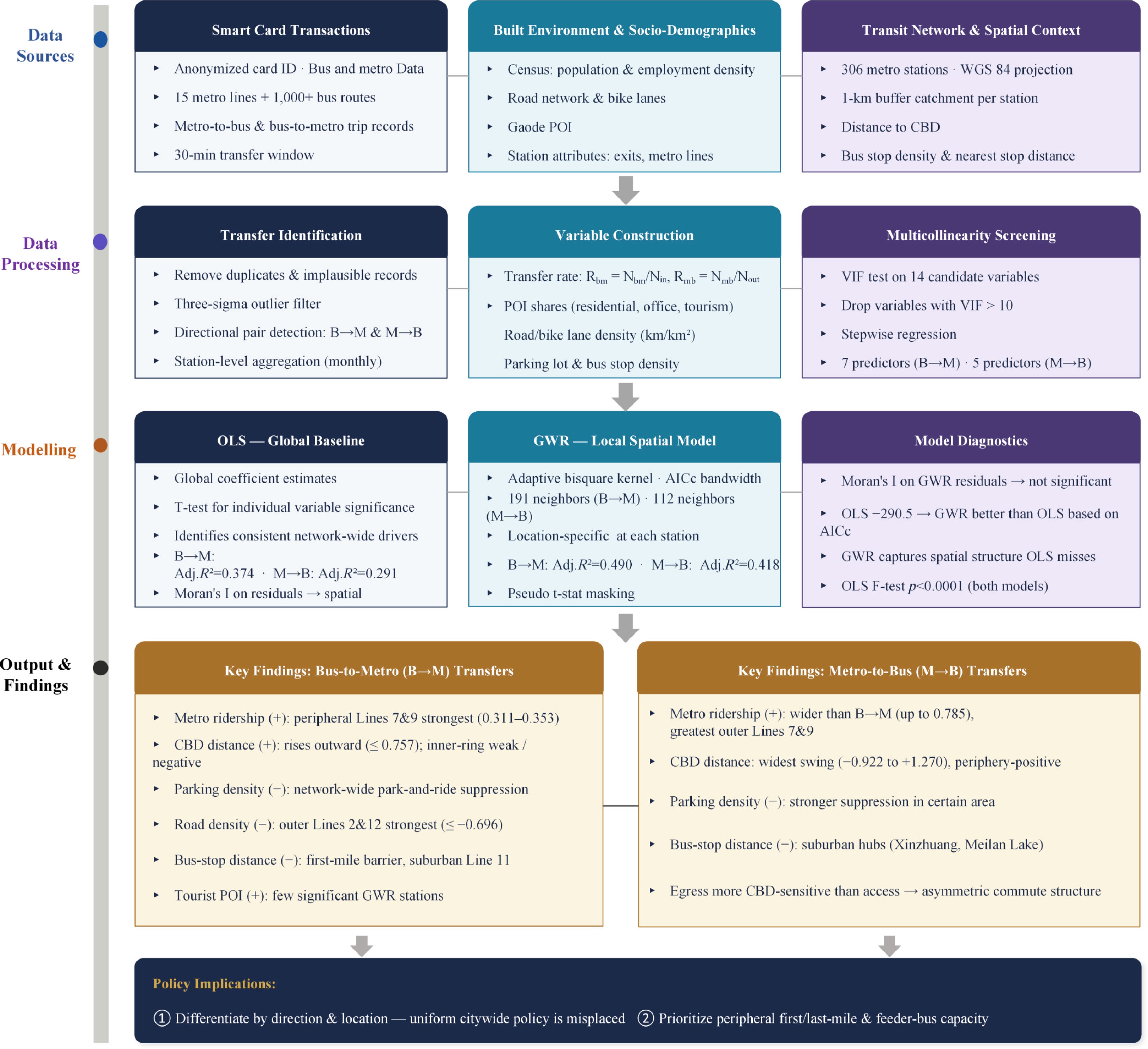
Figure 1.
General research framework for analyzing spatial heterogeneity in metro–bus transfer behavior.
Study area and data
-
Shanghai, the most populous metropolis in China, is a premier case for studying metro–bus integration. Covering 6,340 km2 with 16 districts[2], it remains one of China's largest and densest municipalities, making it an exemplary case for examining metro–bus integration. The city has committed to green and low-carbon transportation in its 2017–2035 master plan, which emphasizes transit network optimization and the construction of a multimodal rail transit system[21]. As of the mid-2010s, Shanghai operated one of the world's largest public transport systems[22], with a vast metro network (15 lines in 2015) and an extensive bus system (over 1,000 routes). This study leverages multiple data sources from Shanghai to analyze metro–bus transfer ridership. The primary dataset is transit smart card transactions recorded in April 2015[2], encompassing all metro and bus rides in the city during that month. This 1-month smart card dataset captures millions of rides across the 15 metro lines and 1,000+ bus routes, with each record containing an anonymized card ID, date, time, mode (metro or bus), route/station name, and fare paid. These detailed electronic records provide sequential trip information that can reveal when and where passengers transfer between the metro and bus.
To strengthen the analysis of metro–bus transfer behavior, we complemented the smart card dataset with a comprehensive built-environment database around transit stations. This included socio-demographic data from the national census (population and employment counts)[23], the street network from OpenStreetMap (OSM)[24], and POI data collected from Gaode Maps[25] (2015). The POI dataset classifies locations into 15 categories such as dining, retail, residential communities, offices, schools, hospitals, tourist attractions, and transportation facilities, providing a detailed representation of local land-use characteristics. In addition, key characteristics of each metro station's facilities—particularly the number of metro lines serving the station and the number of station entrances/exits—were obtained from official transit agency records. All data sources were standardized to a consistent spatial and temporal scope. Specifically, all spatial datasets were projected to the WGS 84 coordinate system, and the temporal coverage was restricted to April 2015, during which 1 month of metro and bus smart card transactions, along with corresponding built-environment data, were collected and aligned for analysis. Built-environment indicators were calculated within a 1 km buffer around each metro station, as this distance is commonly adopted in transit research to approximate typical walking catchment areas and to capture the immediate spatial context influencing transfer behavior. This integration of smart card transactions with built environment and transport-related attributes ensured a robust multi-source database for subsequent empirical analysis.
Data processing
-
All datasets underwent rigorous preprocessing to ensure quality and consistency. The raw smart card data were first cleaned by removing incomplete records and duplicates. Implausible entries, such as trips with erroneous timestamps or unrealistic durations, were filtered out. In addition, a geographic boundary filter was applied to retain only trips occurring within the Shanghai metropolitan area. To further ensure reliability, outlier detection was conducted on trip durations and distances, and any journeys exceeding three standard deviations from the mean were excluded. This 'three-sigma' approach, commonly used in transport data analysis, prevented unusually long or erroneous trips from distorting subsequent modeling. After these cleaning steps, a refined dataset of smart card transactions was obtained, containing temporally and spatially consistent records of metro and bus trips.
While the empirical analysis is based on the April 2015 smart card dataset, several considerations support its continued analytical validity. First, this dataset offers a complete network-wide census of all metro and bus transactions, with strict temporal alignment to contemporaneous census, OpenStreetMap, and Gaode POI data—a level of cross-source consistency that is essential for unbiased GWR estimation but increasingly difficult to achieve with recent datasets due to tightened data governance regulations in China. Second, the principal contribution of this study lies in identifying spatial heterogeneity mechanisms in metro–bus transfer behavior rather than in providing point estimates for current operational planning; the underlying core–periphery structure of Shanghai's transit system has been structurally preserved despite network expansion. Although new metro lines have been added since 2015, these extensions have predominantly increased peripheral coverage rather than altered the dense central network, and may in fact have reinforced the core–periphery gradient documented in our results. Recent studies using post-2018 Shanghai data report consistent spatial patterns[26].
In this study, a metro–bus combined trip is defined as a journey in which a passenger uses metro and bus sequentially, linked by a transfer within a short time window. Because smart card systems log discrete boarding and alighting events rather than complete travel chains, identifying such linked journeys requires a maximum elapsed-time rule to separate an interchange from the start of a new journey[5,27]. Following the thresholds commonly adopted in smart card studies of multimodal transfer behavior[27], we set this window to 30 min: where a passenger exited one mode and boarded the other within 30 min, the two segments were treated as a single continuous journey involving a transfer. Among passengers departing from a metro station, some continue via metro, while others switch to buses. Metro-to-bus transfers were identified and retained by examining the travel mode field in the trip dataset, with transfer times capped at 30 min. This method applies equally to identifying bus-to-metro transfers. The overall structure of this metro–bus transfer process is illustrated in Fig. 2.
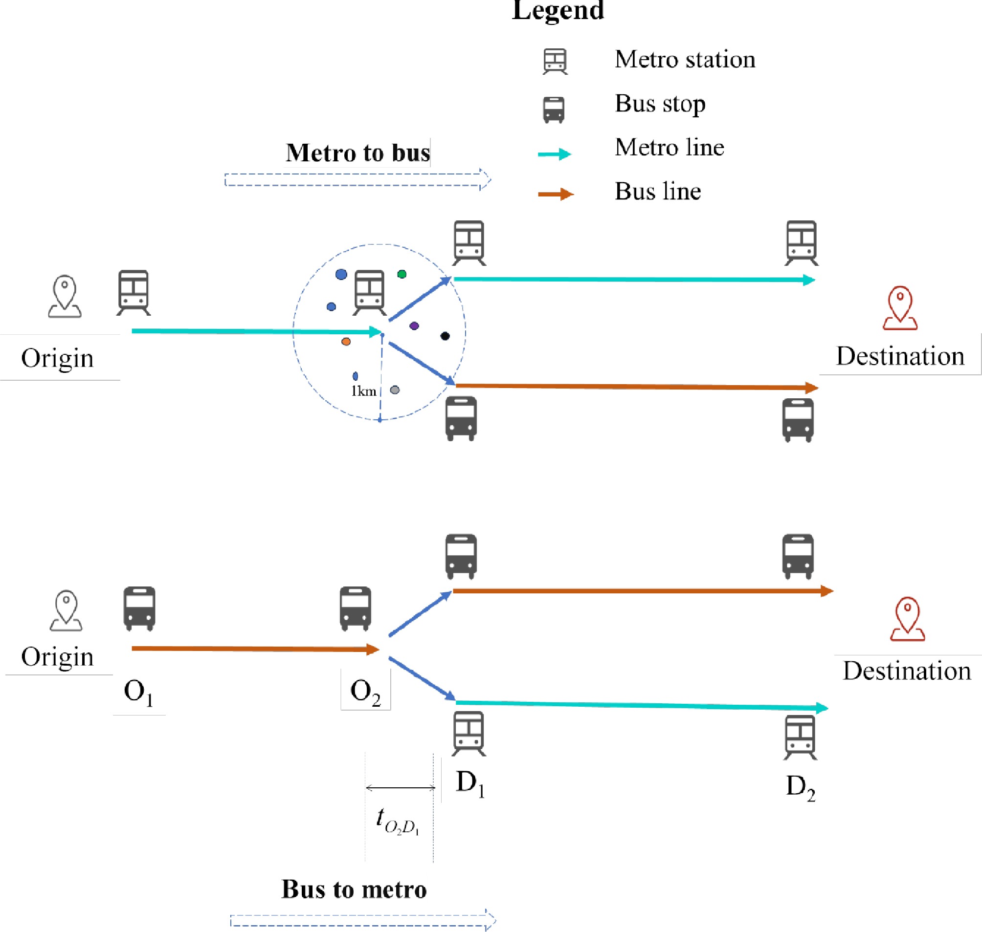
Figure 2.
Defining a metro–bus transfer: a 30-min window linking trip legs across modes.
In parallel, a series of built-environment measures was derived to quantify the spatial context of transfers. As illustrated in the upper panel of Fig. 2, a circular buffer zone with a 1 km radius was established around each metro station. Within this zone, POIs, road segments, and census data were aggregated. From these inputs, we calculated land-use indicators (the proportion of residential, office, and tourism POIs), road network density (km/km2), and bicycle lane density. Socio-demographic attributes, including population density and employment density, were derived from census data for the corresponding areas. All built-environment and socio-demographic attributes were then linked to the station-level transfer data. Table 1 reports descriptive statistics of the key variables after processing.
Table 1. Definitions and descriptive statistics of the variables.
Category Variable Symbol Min Mean Max SD Dependent variables Bus$ \rightarrow $Metro transfer rate $ R_{{{\mathrm{B}}\to {\mathrm{M}}}} $ (ratio) 0.000296 0.122 0.696 0.123 Metro$ \rightarrow $Bus transfer rate $ R_{{{\mathrm{M}}\to {\mathrm{B}}}} $ (ratio) 0.000132 0.113 0.803 0.118 Transit service and station network Metro ridership (monthly) $ MR $ (#) 1,171 436,923 2,567,207 387,063 Number of metro lines $ N_{\text{line}} $ (lines) 1 1.310 4 0.621 Number of station exits $ N_{\text{exit}} $ (#) 1 5.143 20 2.826 Distance to nearest bus stop $ D_{\text{bus\_nn}} $ (km) 0.003 0.256 1.872 0.326 Bus stop density $ D_{\text{bus}} $ (#/km2) 0 7.065 15.924 3.153 Built environment Parking density $ D_{\text{par}} $ (#/km2) 0 5.118 13.113 3.771 Bicycle lane density $ D_{\text{bld}} $ (km/km2) 0 0.452 4.023 0.863 Road network density $ D_{\text{road}} $ (km/km2) 0.036 12.791 32.331 5.540 Distance to CBD $ D_{\text{CBD}} $ (km) 0.552 13.735 65.984 10.324 Residential POI share $ P_{\text{res}} $ (ratio) 0.215 0.472 0.798 0.096 Office POI share $ P_{\text{off}} $ (ratio) 0 0.101 0.288 0.029 Tourism POI share $ P_{\text{tour}} $ (ratio) 0 0.328 0.667 0.060 Population density (buffer) $ P_{\text{pop}} $ (pers/km2) 56 18,851.271 44,682 12,126.491 Employment density (buffer) $ P_{\text{job}} $ (jobs/km2) 0.080 285.476 905.573 246.295 SD, standard deviation; POI, point of interest; CBD, central business district. #, number (count). Transfer rates and POI shares are expressed as ratios (0–1), not percentages. Metro ridership is the total number of entries recorded at the station over the 1-month study period (April 2015). All built-environment and socio-demographic indicators are measured within a 1 km buffer around each metro station. Variable descriptions
-
To investigate the determinants of metro–bus transfer ridership in Shanghai, explanatory variables were drawn from three dimensions: transportation and travel characteristics, built environment and land-use attributes, and population and employment factors. These perspectives capture both the supply side of transit services and the demand side of urban activity distribution. Two dependent variables were defined: the B
$ \rightarrow $ $ \rightarrow $ Transportation and travel characteristics
-
Metro station ridership serves as an indicator of a station's role within the urban public transport network. High passenger volumes not only reflect strong dependence on rail transit but also place greater demands on bus feeder capacity. Accordingly, metro ridership is included as a variable in analyzing bus–metro integration. The number of metro lines and station entrances/exits further shape transfer convenience: a higher number of lines enhances connectivity and expands the catchment area, whereas multiple entrances/exits facilitate passenger dispersion and reduce bottlenecks during transfers. The spatial relationship between metro and bus stops also plays a critical role. The distance to the nearest bus stop determines the walking cost of a transfer: shorter distances encourage combined metro–bus use, while longer distances discourage passengers and increase the likelihood of modal substitution. Similarly, bus stop density captures the overall supply of feeder services; higher densities generally provide more transfer opportunities but may also be associated with operational complexity.
Built-environment and land-use characteristics
-
Several indicators were introduced to represent how the urban form influences transfer behavior. The distance from a station to the central business district (CBD) reflects the spatial structure of commuting flows, with centrally located stations typically attracting more access trips. Parking lot density measures the degree of automobile accessibility, which may substitute for feeder buses in suburban contexts by encouraging park-and-ride trips. Bicycle lane density is included as a competing access mode; where safe and continuous cycling infrastructure exists, passengers may rely less on bus feeders for metro access. Road network density, defined as road length per unit area, represents connectivity and route diversity. A denser network can increase accessibility but may also dilute feeder bus demand by providing alternative travel paths. Land-use attributes are represented through the share of specific POIs (tourist, office, and residential functions) within the station catchment. Tourist and office-related POIs typically generate strong directional transfer demand (e.g., egress trips in the morning or access trips for leisure), while residential POIs reflect potential origins of feeder demand.
Population density reflects the residential base of potential metro users who may rely on feeder buses for access, while employment density represents workplace concentration that generates egress trips. Unlike office POIs, which capture a specific land-use type, employment density broadly reflects job opportunities across industries, providing a more general measure of work-related travel demand. These two demographic indicators complement land-use variables by quantifying the scale of local demand for multimodal transfers.
Dependent variables
-
To avoid biases caused by absolute ridership volumes, transfer efficiency is captured by directional rates using 1 month of data. The bus-to-metro transfer rate is defined as:
$ R_{{\mathrm{B}} \rightarrow {\mathrm{M}}} = \dfrac{N_{{\mathrm{B}} \rightarrow {\mathrm{M}}}}{N_{\text{in}}} $ (1) where,
$ N_{{\mathrm{B}} \rightarrow {\mathrm{M}}} $ $ N_{\text{in}} $ The metro-to-bus transfer rate is defined as:
$ R_{{\mathrm{M}} \rightarrow {\mathrm{B}}} = \dfrac{N_{{\mathrm{M}} \rightarrow {\mathrm{B}}}}{N_{\text{out}}}$ (2) where,
$ N_{{\mathrm{M}} \rightarrow {\mathrm{B}}} $ $ N_{\text{out}} $ These directional rates measure the proportion of metro users at each station who rely on bus integration for access (
$ R_{{\mathrm{B}} \rightarrow {\mathrm{M}}} $ $ R_{{\mathrm{M}} \rightarrow {\mathrm{B}}} $ In summary, the selected variables comprehensively capture station-level transfer dynamics across three dimensions: service supply (metro and bus characteristics), built-environment conditions (land use, infrastructure, and urban form), and socio-demographic context (residential and employment density). Table 1 presents descriptive statistics for all variables measured at 306 metro stations in April 2015. Prior to estimation, all explanatory variables were rescaled to a common numerical range so that the estimated coefficients are directly comparable in magnitude across predictors; the dependent transfer rates were retained on their original 0–1 scale.
-
This study employs GWR and OLS models to examine how built-environment variables influence metro–bus transfer rates. To ensure model robustness, the VIF test was first applied to the 14 explanatory variables, thereby addressing potential multicollinearity and improving estimation reliability. Subsequently, a stepwise regression procedure was conducted to retain only statistically significant variables. This process reduced redundancy among predictors and ensured that the final models focused on the most relevant determinants of
$ R_{{\mathrm{B}} \rightarrow {\mathrm{M}}} $ $ R_{{\mathrm{M}} \rightarrow {\mathrm{B}}} $ Multicollinearity test
-
Before estimating the regression models, it is essential to ensure that explanatory variables are not strongly correlated with one another, as multicollinearity may bias coefficient estimates and reduce the reliability of statistical inference. To address this issue, the variance inflation factor (
$ VIF $ $ VIF $ $ R^{2} $ $ VIF = \dfrac{1}{1 - R^{2}} $ (3) A commonly used threshold is
$ VIF \gt 10 $ Ordinary least squares
-
To examine the global determinants of bus–metro transfer rates, we employed the OLS regression model as a baseline analytical framework[29]. The dependent variables were defined as the
$ R_{{\mathrm{M}} \rightarrow {\mathrm{B}}} $ $ R_{{\mathrm{B}} \rightarrow {\mathrm{M}}} $ The OLS model is specified as:
$ Y_i = \beta_0 + \sum_{k=1}^{p} \beta_k X_{ik} + \varepsilon_i, \quad i=1,2,\cdots,n, $ (4) where
$ Y_i $ $ R_{{\mathrm{M}} \rightarrow {\mathrm{B}}} $ $ R_{{\mathrm{B}} \rightarrow {\mathrm{M}}} $ $ i $ $ X_{ik} $ $ k $ $ i $ $ \beta_k $ $ \varepsilon_i $ Stepwise regression
-
To identify the most influential explanatory variables, stepwise regression was employed prior to model estimation. This procedure iteratively introduces or eliminates candidate variables based on the
$ F $ $ R_{{\mathrm{B}} \rightarrow {\mathrm{M}}} $ $ R_{{\mathrm{M}} \rightarrow {\mathrm{B}}} $ The decision criterion for stepwise selection is based on the
$ F $ $ F = \dfrac{(RSS_{r} - RSS_{ur})\,/\,(p_{ur} - p_{r})}{RSS_{ur}\,/\,(n - p_{ur} - 1)} $ (5) where,
$ RSS_{r} $ $ RSS_{ur} $ $ p_{r} $ $ p_{ur} $ $ n $ $ F $ Spatial autocorrelation test
-
Before applying the GWR, the spatial dependence of the global model residuals is examined, since residual spatial autocorrelation indicates that a global specification has failed to capture spatially varying relationships[30]. Moran's
$ I $ In this study, Moran's
$ I $ $ I $ $ I = \dfrac{n}{W} \cdot \dfrac{ \displaystyle\sum_{i=1}^{n}\displaystyle\sum_{j=1}^{n} w_{ij}(x_i - \bar{x})(x_j - \bar{x})} { \displaystyle\sum_{i=1}^{n}(x_i - \bar{x})^2} $ (6) where,
$ n $ $ x_i $ $ x_j $ $ x $ $ i $ $ j $ $ \bar{x} $ $ x $ $ w_{ij} $ $ i $ $ j $ $ W = \displaystyle\sum_i\displaystyle\sum_j w_{ij} $ If the test results indicate significant positive spatial autocorrelation, global OLS estimates may fail to capture localized spatial processes. In such cases, local models such as GWR are necessary to account for spatial heterogeneity and to provide more accurate inference.
Geographically weighted regression model
-
In regression analysis, if linear regression models are used without accounting for spatial context, the estimated coefficients may ignore spatial non-stationarity and fail to capture the true underlying relationships[30]. Specifically, the association between independent variables and dependent outcomes often varies across space, reflecting localized dynamics rather than global uniformity. Ignoring this heterogeneity can obscure important insights and lead to biased inferences. In the context of this study, spatial non-stationarity is particularly relevant for analyzing metro–bus transfer rates, where built environment factors may exert different effects in central versus peripheral districts[14]. To address this issue, we adopt GWR, which extends the traditional OLS model by allowing coefficients to vary across geographic space.
The GWR model can be expressed as:
$ Y_i = \beta_0(u_i,v_i) + \sum_{k=1}^{p}\beta_k(u_i,v_i)\,X_{ik} + \varepsilon_i, \quad i=1,2,\cdots,n $ (7) where,
$ (u_i,v_i) $ $ i $ $ \beta_k(u_i,v_i) $ $ k $ $ \varepsilon_i $ The coefficients are estimated using a weighted least squares procedure:
$ \hat{\beta}(u_i,v_i) = \bigl(X^{\top} W(u_i,v_i)\,X\bigr)^{-1} X^{\top} W(u_i,v_i)\,Y $ (8) where,
$ X $ $ \begin{array}{l} X = \begin{bmatrix} 1 & x_{11} & \cdots & x_{1k} \\ 1 & x_{21} & \cdots & x_{2k} \\ \vdots & \vdots & \ddots & \vdots \\ 1 & x_{n1} & \cdots & x_{nk} \end{bmatrix}, \end{array} $ (9) $ W(u_i,v_i) $ $ W(u_i,v_i) = \operatorname{diag}\bigl\{ w_{1}(u_i,v_i),\, w_{2}(u_i,v_i),\,\ldots,\, w_{n}(u_i,v_i) \bigr\}. $ (10) In this study, an adaptive bisquare kernel function was employed to construct the spatial weight matrix. The weight assigned to observation
$ j $ $ i $ $ w_{ij} = \left\{\begin{aligned} &\left[1 - \left(\dfrac{d_{ij}}{b_i}\right)^2\right]^2, && \text{if } d_{ij} \lt b_i &\\ &0, && \text{otherwise}& \end{aligned}\right. $ (11) where,
$ d_{ij} $ $ i $ $ j $ $ b_i $ $ i $ $ \rightarrow $ $ \rightarrow $ $ \beta $ $ \begin{array}{l} \beta = \begin{bmatrix} \beta_0(u_1,v_1) & \cdots & \beta_k(u_1,v_1) \\ \beta_0(u_2,v_2) & \cdots & \beta_k(u_2,v_2) \\ \vdots & \ddots & \vdots \\ \beta_0(u_n,v_n) & \cdots & \beta_k(u_n,v_n) \end{bmatrix}, \end{array} $ (12) and
$ Y $ $ \begin{array}{l} Y = \begin{bmatrix} y_1 \\ y_2 \\ \vdots \\ y_n \end{bmatrix}. \end{array} $ (13) By systematically comparing OLS and GWR, we evaluate both global and spatially varying determinants of transfer ridership.
-
This section presents the empirical findings of the study. Global regression results provide baseline associations between explanatory variables and transfer rates, while GWR highlights spatial heterogeneity in their effects. The discussion is organized to compare bus-to-metro and metro-to-bus transfers, emphasizing both common patterns and location-specific variations.
Model diagnostics and specification
-
The diagnostic procedure began with multicollinearity screening of all explanatory variables listed in Table 1. The VIF was computed using ArcGIS, and variables with VIF values above 10 were excluded to ensure model stability. After this filtering, stepwise OLS regressions were conducted separately for
$ R_{{\mathrm{M}} \rightarrow {\mathrm{B}}} $ $ R_{{\mathrm{B}} \rightarrow {\mathrm{M}}} $ $ R_{{\mathrm{B}} \rightarrow {\mathrm{M}}} $ $ R_{{\mathrm{M}} \rightarrow {\mathrm{B}}} $ Following the stepwise OLS regression, and based on the specification of the OLS model in Eq. (4), the final regression equations for
$ R_{{\mathrm{B}} \rightarrow {\mathrm{M}}} $ $ R_{{\mathrm{M}} \rightarrow {\mathrm{B}}} $ $ \begin{aligned} \hat{R}_{{{\mathrm{B}}\to {\mathrm{M}}}} =& \beta_0 - 0.029\,P_{\text{pop}} + 0.230\,D_{\text{CBD}} + 0.319\,P_{\text{tour}} \\ &- 0.137\,D_{\text{par}} - 0.139\,D_{\text{road}} + 0.154\,MR - 0.074\,D_{{\text{bus}}\_{\mathrm{nn}}} \end{aligned} $ (14) where,
$ R_{{{\mathrm{B}}\to {\mathrm{M}}}} $ $ P_{\text{tour}} $ $ P_{\text{pop}} $ $ D_{\text{CBD}} $ $ D_{\text{par}} $ $ D_{\text{road}} $ $ MR $ $ D_{{\text{bus}}\_{\mathrm{nn}}} $ $ D_{\text{CBD}} $ $ P_{\text{tour}} $ $ MR $ $ R_{{{\mathrm{B}}\to {\mathrm{M}}}} $ $ P_{\text{pop}} $ $ D_{\text{par}} $ $ D_{\text{road}} $ $ D_{{\text{bus}}\_{\mathrm{nn}}} $ $ \begin{aligned} \hat{R}_{{{\mathrm{M}}\to {\mathrm{B}}}} =& \beta_0 - 0.048\,P_{\text{pop}} + 0.336\,D_{\text{CBD}} - 0.160\,D_{\text{par}} \\ &- 0.123\,D_{{\text{bus}}\_{\mathrm{nn}}} + 0.266\,MR \end{aligned} $ (15) where,
$ R_{{{\mathrm{M}}\to {\mathrm{B}}}} $ $ P_{\text{pop}} $ $ D_{\text{CBD}} $ $ D_{\text{par}} $ $ D_{{\text{bus}}\_{\mathrm{nn}}} $ $ MR $ $ P_{\text{pop}} $ $ D_{\text{par}} $ $ D_{{\text{bus}}\_{\mathrm{nn}}} $ $ R_{{{\mathrm{M}}\to {\mathrm{B}}}} $ $ D_{\text{CBD}} $ $ MR $ To further examine the significance of individual explanatory variables, t-tests were conducted on the OLS regression coefficients. Unlike the
$ F $ $ \alpha=0.05 $ $ \alpha=0.10 $ Table 2. OLS coefficient estimates and t-tests ($ R_{{\mathrm{B}} \rightarrow {\mathrm{M}}} $).
Variable Coefficient t-statistic p-value Significance Road network density −0.139395 −2.187172 0.029495 ** Distance to nearest bus stop −0.074204 −1.864957 0.063174 * Distance to CBD 0.230025 3.210951 0.001468 *** Population densitya −0.029297 −0.622181 0.534300 ns Proportion of tourist POIs 0.318515 2.044617 0.041763 ** Parking density −0.136822 −3.438710 0.000681 *** Metro ridership 0.154115 3.837729 0.000161 *** ***, **, and * indicate that the coefficient is statistically significant at the 1%, 5%, and 10% levels, respectively (i.e., p < 0.01, p < 0.05, and p < 0.10); ns indicates not significant (p ≥ 0.10). a Population density was retained in the OLS results for transparency, but excluded from the GWR estimation due to its insignificant OLS t-statistic. Table 3. OLS coefficient estimates and t-tests ($ R_{{\mathrm{M}} \rightarrow {\mathrm{B}}} $).
Variable Coefficient t-statistic p-value Significance Distance to CBD 0.336207 2.407780 0.016641 ** Population density −0.047775 −0.761604 0.446886 ns Distance to nearest bus stop −0.122878 −2.490553 0.013285 ** Parking density −0.160087 −3.049310 0.002507 *** Metro ridership 0.266319 4.689708 0.000006 *** ***, **, and * indicate that the coefficient is statistically significant at the 1%, 5%, and 10% levels, respectively (i.e., p < 0.01, p < 0.05, and p < 0.10); ns indicates not significant (p ≥ 0.10). Prior to estimating the GWR models, the spatial dependence of the OLS residuals was examined using the global Moran's
$ I $ $ \rightarrow $ $ I $ $ \rightarrow $ $ I $ Table 4. Global Moran's $ I $ test on OLS residuals.
Model Moran's $ I $ $ Z $-score p-value Significance OLS (B$ \rightarrow $M) 0.113058 4.451014 < 0.00001 *** OLS (M$ \rightarrow $B) 0.123467 4.858613 < 0.00001 *** ***, **, and * indicate statistical significance at the 1%, 5%, and 10% levels, respectively; ns indicates not significant (p ≥ 0.10). Following GWR estimation, residual spatial autocorrelation is substantially reduced and rendered statistically insignificant in both cases, as reported in Table 5. Moran's
$ I $ $ \rightarrow $ $ \rightarrow $ Table 5. Global Moran's $ I $ test on GWR residuals.
Model Moran's $ I $ $ Z $-score p-value Significance GWR (B$ \rightarrow $M) −0.003062 0.016194 0.987079 ns GWR (M$ \rightarrow $B) −0.012077 −0.632434 0.527103 ns ***, **, and * indicate statistical significance at the 1%, 5%, and 10% levels, respectively; ns indicates not significant (p ≥ 0.10). The p-values of population density (0.534300 and 0.446886, respectively) fail to reach statistical significance, indicating that its effect on the dependent variable is not significant. Therefore, this variable was excluded from the GWR model. It is worth noting that the application of the global Moran's
$ I $ $ I $ After retaining the significant explanatory variables, a spatial autocorrelation test was conducted. Specifically, the global Moran's
$ I $ $\mathrm{ArcGIS} $ $ I $ $ Z $ $ Z $ Table 6. Moran's $ I $ test for spatial autocorrelation ($ R_{{\mathrm{B}} \rightarrow {\mathrm{M}}} $).
Variable Moran's $ I $ Expected index $ Z $-score p-value Significance Metro ridership 0.258069 −0.003279 10.05420 < 0.000001 *** Distance to nearest bus stop 0.452975 −0.003279 17.57602 < 0.000001 *** Distance to CBD 0.957835 −0.003279 36.96441 < 0.000001 *** Population density 0.786053 −0.003279 30.08828 < 0.000001 *** Tourist POI proportion 0.383708 −0.003279 15.59166 < 0.000001 *** Road network density 0.646344 −0.003279 24.85657 < 0.000001 *** Parking lot density 0.693274 −0.003279 24.90747 < 0.000001 *** ***, **, and * indicate statistical significance at the 1%, 5%, and 10% levels, respectively; ns indicates not significant (p ≥ 0.10). Table 7. Moran's $ I $ test for spatial autocorrelation ($ R_{{\mathrm{M}} \rightarrow {\mathrm{B}}} $).
Variable Moran's $ I $ Expected index $ Z $-score p-value Significance Metro ridership 0.258069 −0.003279 10.05420 < 0.000001 *** Distance to CBD 0.957835 −0.003279 36.96441 < 0.000001 *** Parking lot density 0.693274 −0.003279 24.90747 < 0.000001 *** Distance to nearest bus stop 0.452975 −0.003279 17.57602 < 0.000001 *** Population density 0.786053 −0.003279 30.08828 < 0.000001 *** ***, **, and * indicate statistical significance at the 1%, 5%, and 10% levels, respectively; ns indicates not significant (p ≥ 0.10). Accordingly, GWR models were estimated for both B
$ \rightarrow $ $ \rightarrow $ $ R^{2} $ $ R^{2} $ $ R^{2} $ $ R^{2} $ $ R^2 $ $ \rightarrow $ $ \rightarrow $ $ R^2 $ Table 8. GWR outperforms OLS in explaining bus-to-metro transfer rates ($ R_{{\mathrm{B}} \rightarrow {\mathrm{M}}} $).
Model $ R^{2} $ Adj. $ R^{2} $ AICc $ F $-statistic p-value Significance OLS 0.388 0.374 −438.513 26.992 < 0.000001 *** GWRa 0.548 0.490 −486.286 – – – ***, **, and * indicate statistical significance at the 1%, 5%, and 10% levels, respectively; ns indicates not significant (p ≥ 0.10); '–' indicates not applicable, as the GWR model does not report a global $ F $-statistic. a The GWR model was calibrated with an adaptive bandwidth of 191 neighboring features. Table 9. GWR outperforms OLS in explaining metro-to-bus transfer rates ($ R_{{\mathrm{M}} \rightarrow {\mathrm{B}}} $).
Model $ R^{2} $ Adj. $ R^{2} $ AICc $ F $-statistic p-value Significance OLS 0.303 0.291 −290.548 26.064 < 0.000001 *** GWRa 0.497 0.418 −329.746 – – – ***, **, and * indicate statistical significance at the 1%, 5%, and 10% levels, respectively; ns indicates not significant (p ≥ 0.10); '–' indicates not applicable, as the GWR model does not report a global $ F $-statistic. a The GWR model was calibrated with an adaptive bandwidth of 112 neighboring features. Discussion on the spatially varying effects
-
After multicollinearity screening, stepwise regression, and the OLS t-tests, six explanatory variables were retained in the GWR model with
$ R_{{{\mathrm{B}}\to {\mathrm{M}}}} $ $ R_{{{\mathrm{M}}\to {\mathrm{B}}}} $ To ensure that the spatial patterns depicted in Figs 3−11 reflect only statistically reliable local relationships, pseudo t-statistics were extracted from the GWR output for each station–variable combination. Stations where the absolute value of the local pseudo t-statistic falls below 1.65 (
$ \alpha = 0.10 $ Spatial heterogeneity of bus-to-metro transfers
-
Following variable selection, six predictors were retained for B
$ \rightarrow $ $ \rightarrow $ Distance to the nearest bus stop
-
Where statistically significant, distance to the nearest bus stop exerts a uniformly negative effect on B
$ \rightarrow $ 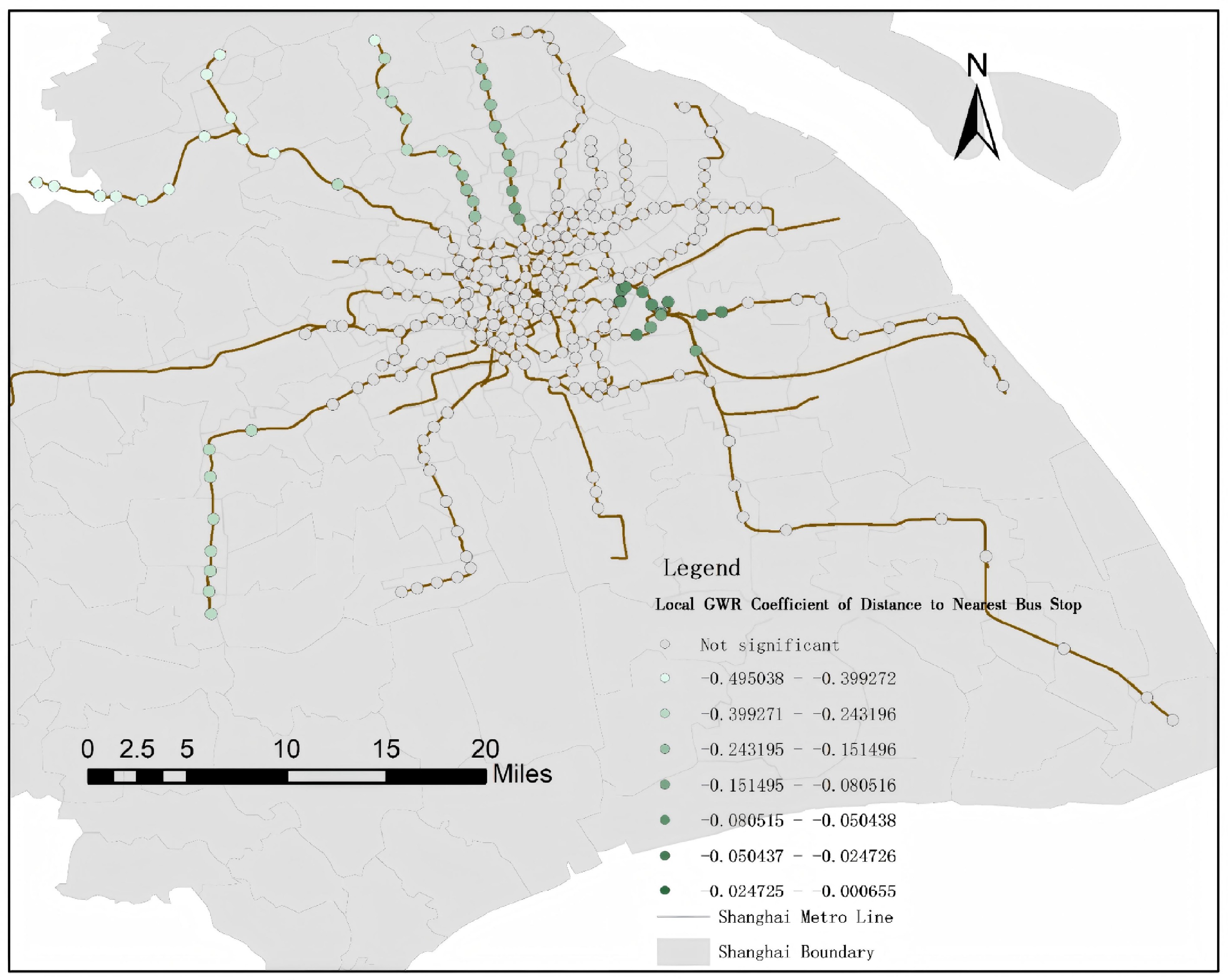
Figure 3.
Local GWR coefficient of nearest bus stop distance on bus-to-metro transfer rates.
Metro ridership
-
Metro ridership is positively associated with B
$ \rightarrow $ 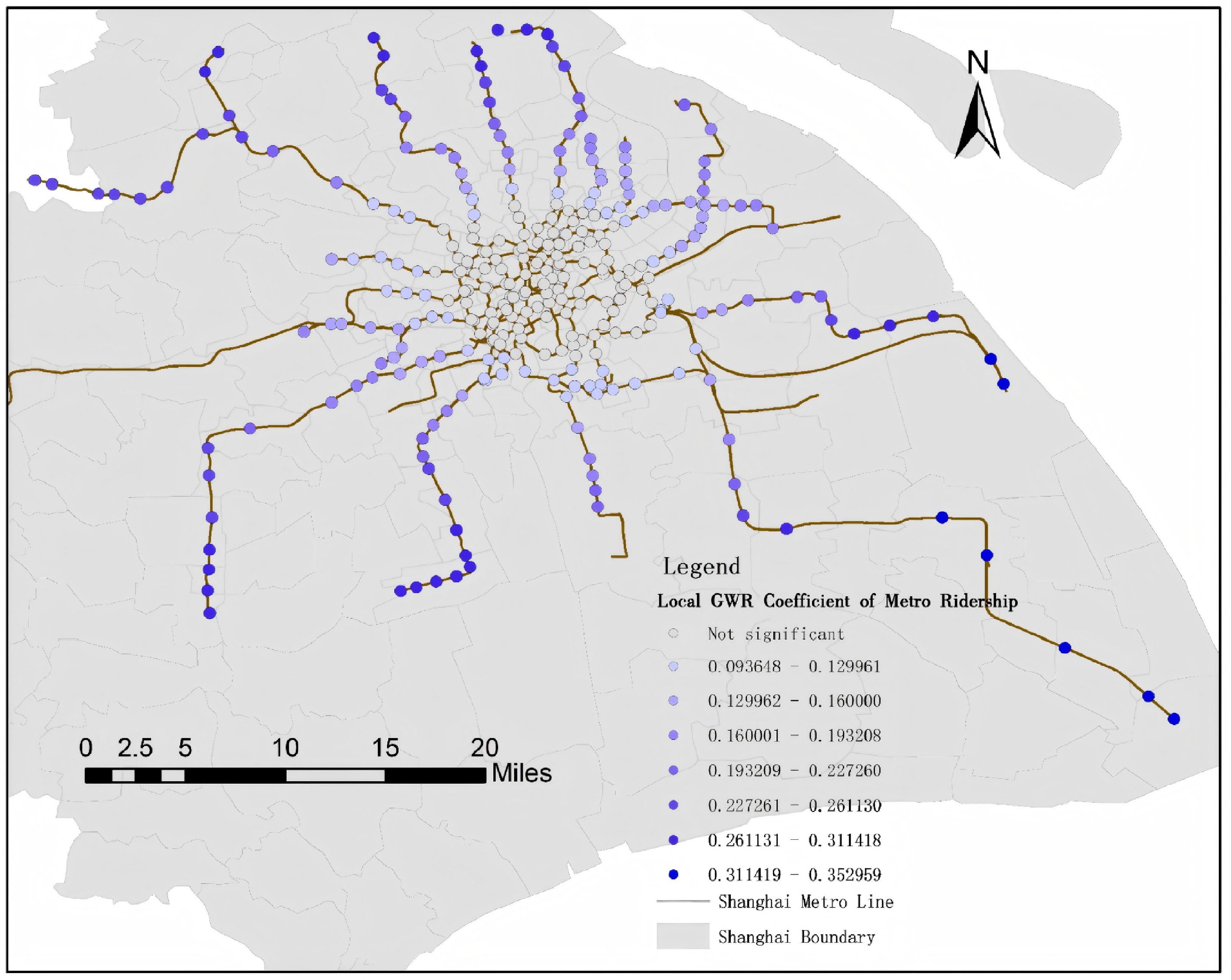
Figure 4.
Local GWR coefficient of metro ridership on bus-to-metro transfer rates.
Road network density
-
Road network density exerts a uniformly negative influence on B
$ \rightarrow $ $ \rightarrow $ 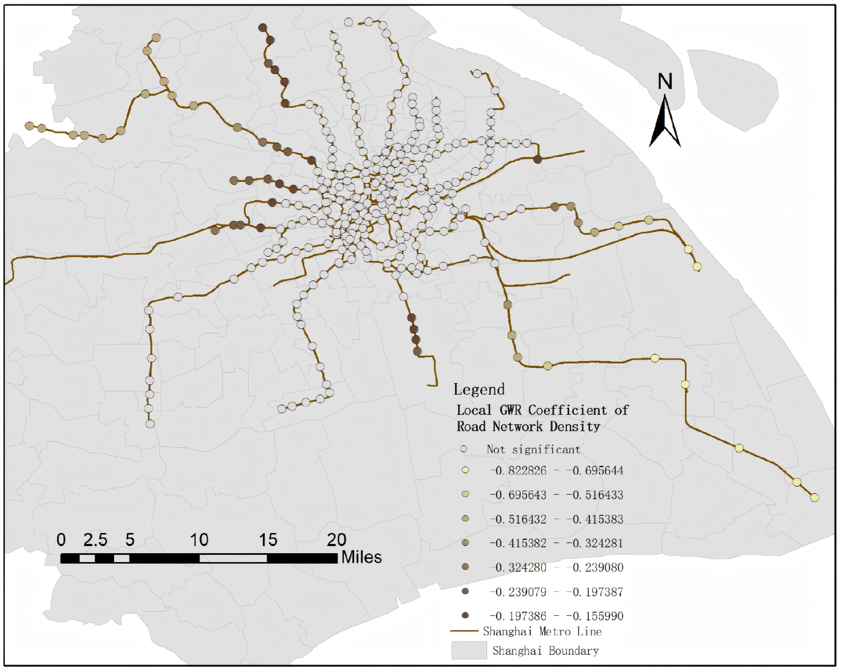
Figure 5.
Local GWR coefficient of road network density on bus-to-metro transfer rates.
Parking density
-
Parking density consistently suppresses B
$ \rightarrow $ $ \rightarrow $ 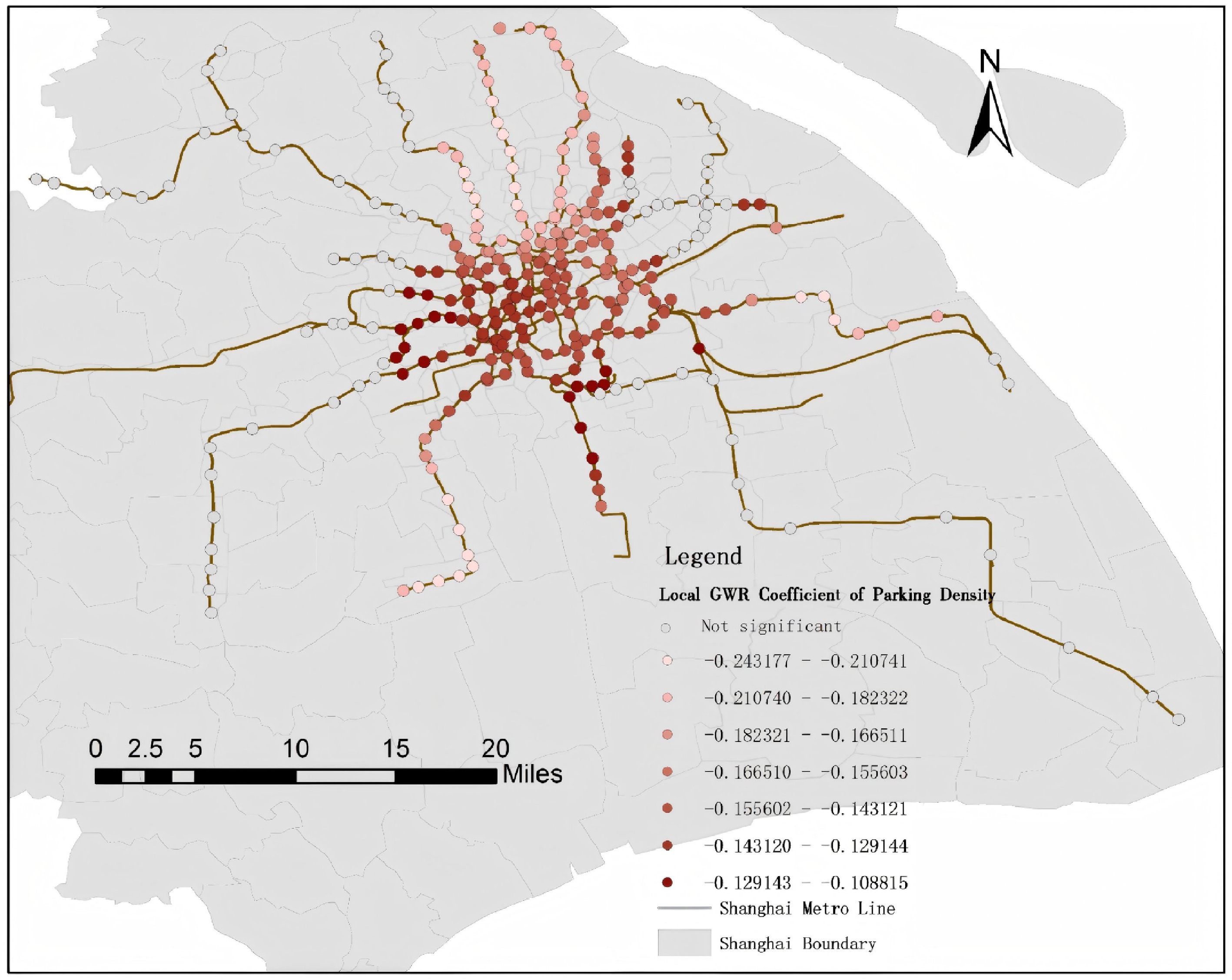
Figure 6.
Local GWR coefficient of parking density on bus-to-metro transfer rates.
Distance to the CBD
-
Distance to the CBD exhibits pronounced spatial heterogeneity in its effect on B
$ \rightarrow $ 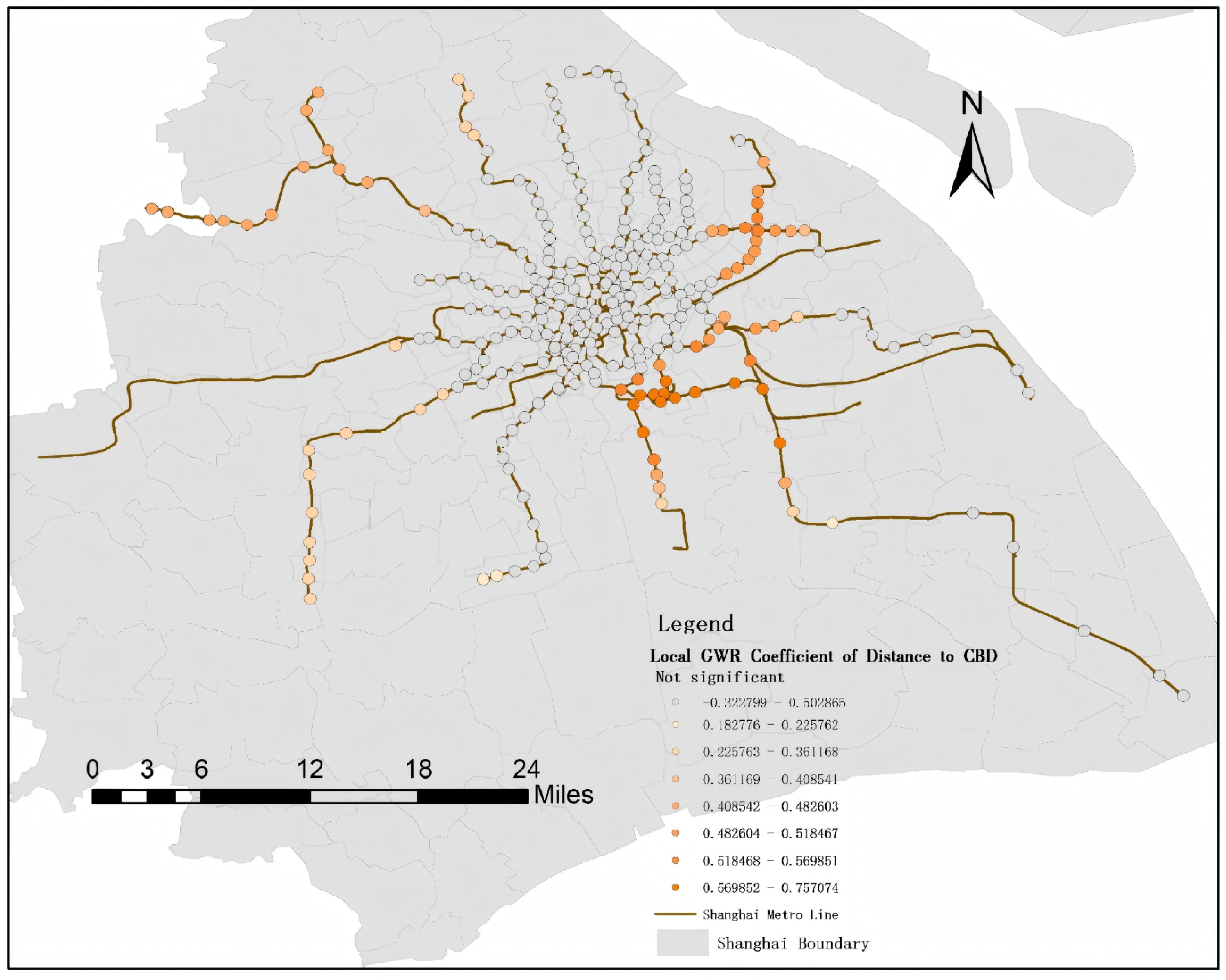
Figure 7.
Local GWR coefficient of distance to CBD on bus-to-metro transfer rates.
Spatial heterogeneity of metro-to-bus transfers
Distance to the nearest bus stop
-
Bus-stop distance exerts a predominantly negative and significant effect on M
$ \rightarrow $ 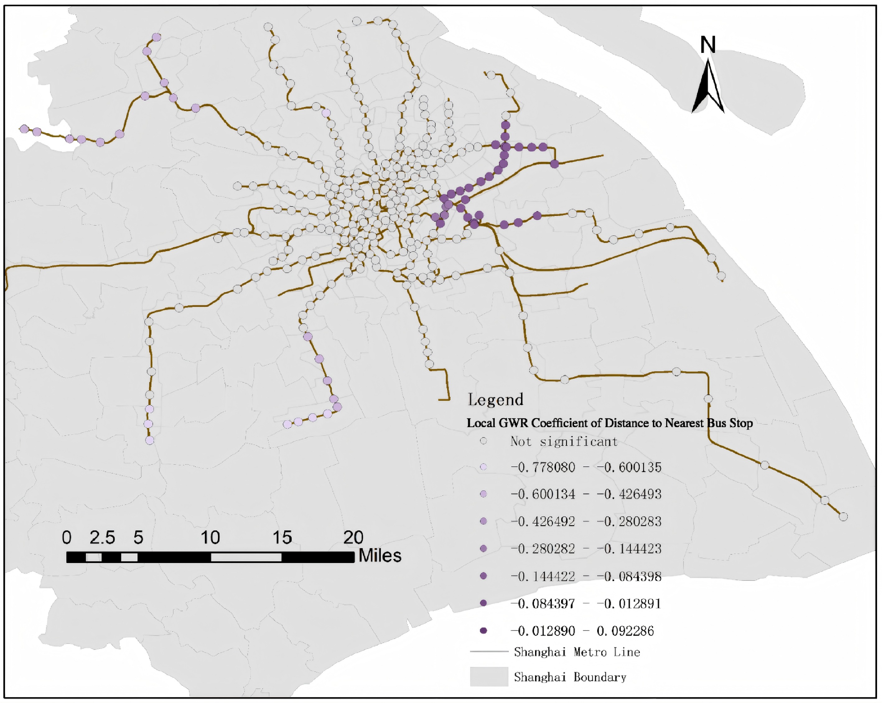
Figure 8.
Local GWR coefficient of distance to nearest bus stop on metro-to-bus transfer rates.
Metro ridership
-
Metro ridership is positively associated with M
$ \rightarrow $ $ \rightarrow $ $ \rightarrow $ 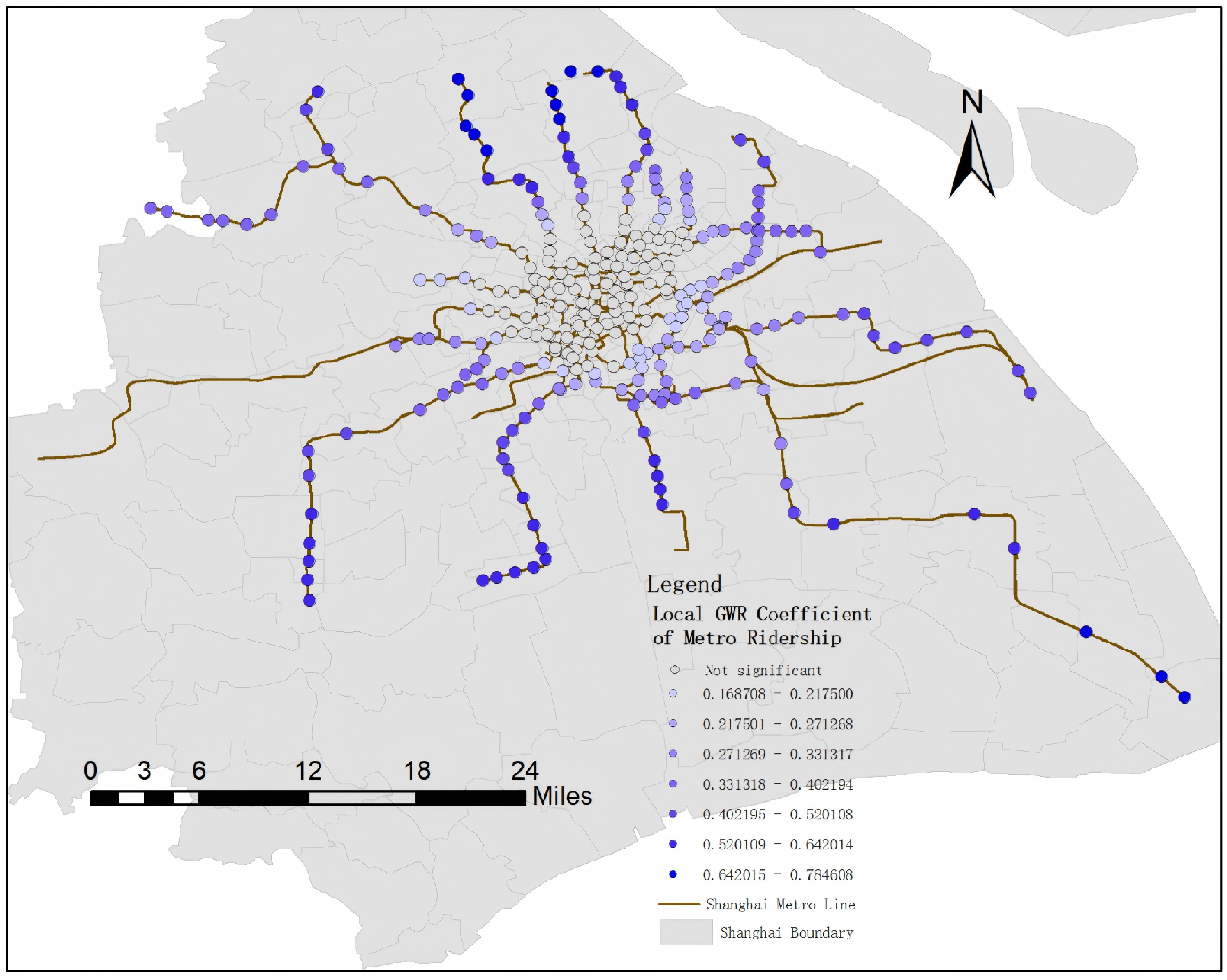
Figure 9.
Local GWR coefficient of metro ridership on metro-to-bus transfer rates.
Parking density
-
Consistent with the negative global association identified in the OLS model, parking density shows a negative local effect on M
$ \rightarrow $ $ \rightarrow $ $ \rightarrow $ 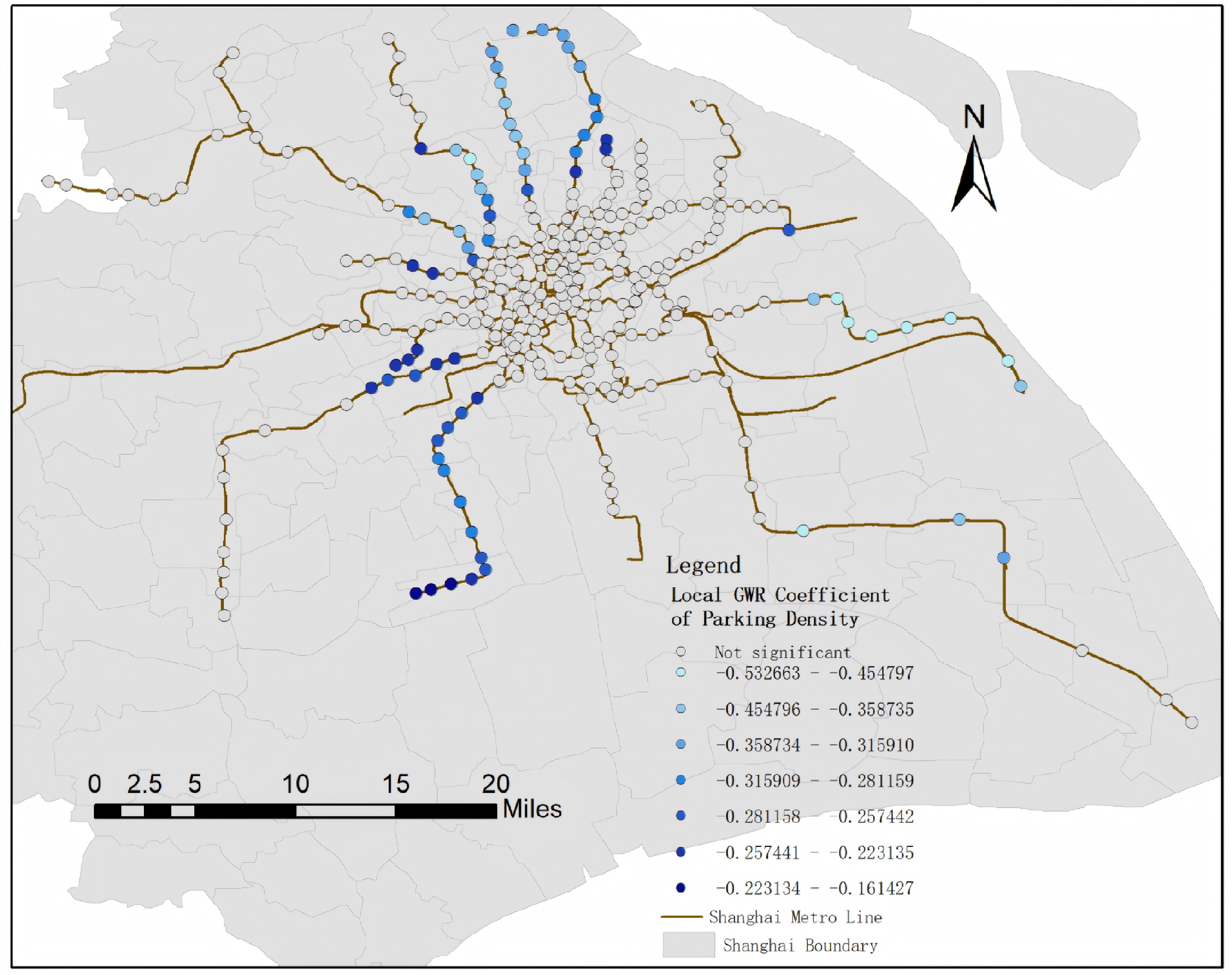
Figure 10.
Local GWR coefficient of parking density on metro-to-bus transfer rates.
This directional asymmetry in parking effects also resonates with a parallel line of inquiry in Shanghai's transfer literature. A study of metro–bus transfer patterns across different station types in central Shanghai used a GTWR-RF approach that first clusters stations by the temporal shape of their transfer ridership before estimating built-environment effects within each cluster[26]. Although this method characterizes spatial heterogeneity through station typology rather than continuous local coefficients, its central finding, that built-environment determinants of transfer ridership differ systematically across station groups rather than operating uniformly across the network, is consistent with the present study's evidence that parking density's effect on M
$ \rightarrow $ Distance to the CBD
-
Distance to the CBD exhibits clear spatial heterogeneity in the M
$ \rightarrow $ $ \rightarrow $ 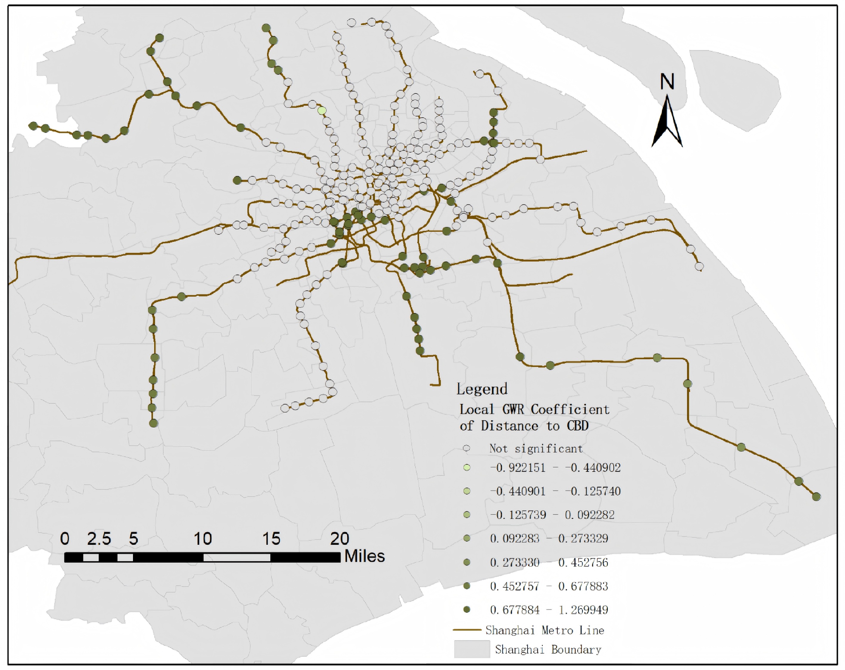
Figure 11.
Local GWR coefficient of distance to CBD on metro-to-bus transfer rates.
-
This study examined the spatially heterogeneous determinants of directional metro–bus transfer rates in Shanghai by integrating 1 month of smart card transactions with station-area built-environment, transit-service, and socio-demographic indicators. By distinguishing B
$ \rightarrow $ $ \rightarrow $ The first major finding is methodological. The significant spatial autocorrelation remaining in the OLS residuals indicates that global coefficients are insufficient for explaining station-level transfer behavior. After applying GWR, residual spatial autocorrelation becomes statistically insignificant, and model fit improves substantially: the adjusted
$ R^2 $ $ \rightarrow $ $ \rightarrow $ Second, the results reveal a clear core–periphery gradient. In peripheral corridors, metro ridership and distance to the CBD generally strengthen reliance on bus feeders or bus egress services, while longer distance to the nearest bus stop creates stronger deterrent effects. In central areas, many local coefficients are weak or statistically insignificant, reflecting dense bus coverage, higher walkability, and more diversified access or egress options. Thus, the same built environment factor may differ in magnitude and statistical significance across urban contexts, and variables such as CBD distance may even exhibit sign changes between central and peripheral areas.
Third, the two transfer directions are governed by related but asymmetric mechanisms. For B
$ \rightarrow $ $ \rightarrow $ $ \rightarrow $ These findings clarify the contributions of the study. Methodologically, this study combines OLS, residual spatial autocorrelation diagnostics, GWR, and pseudo t-statistic masking to distinguish statistically reliable local effects from insignificant coefficient variation. Empirically, it provides station-level evidence that directional metro–bus transfer rates respond differently to built-environment and service-related factors, demonstrating that access and egress transfers should not be treated as a single aggregated outcome. Practically, the results translate spatially varying coefficients into differentiated planning priorities: improving bus-stop proximity and pedestrian transfer conditions at suburban stations, aligning feeder-bus frequency and capacity with metro ridership in peripheral corridors, and coordinating parking management with bus-service planning in automobile-oriented station areas.
Overall, the evidence suggests that metro–bus integration in megacities should be planned as a direction-specific and station-context-specific system. Uniform citywide interventions are unlikely to address the uneven geography of transfer demand; instead, policies should prioritize peripheral and suburban corridors where dependence on bus-based first- and last-mile connections is strongest.
-
Since the 2015 study period, Shanghai's first/last-mile mobility ecosystem has been substantially reshaped by dockless bike-sharing (from 2016 onward) and ride-hailing platforms. Three modifications to the identified patterns are anticipated. First, the deterrent effect of bus-stop distance is likely attenuated in central districts where bike-sharing provides a substitute feeder mode, reinforcing the already near-zero central-core coefficients. In peripheral districts, where bike-sharing supply remains sparse, the sensitivity of transfer demand to bus-stop distance is expected to persist. Second, the suppressive effect of parking density on metro–bus transfers is likely amplified in suburban areas, where ride-hailing further substitutes for bus feeders. Third, the overall core–periphery gradient is expected to persist and possibly intensify, as shared mobility services have themselves developed unevenly, concentrating in central districts. Taken together, emerging mobility modes are likely to modulate rather than overturn the patterns identified here.
While this study provides key insights into the spatial dynamics of metro–bus transfers, its limitations highlight several promising avenues for future research. Future research could extend this work by incorporating high-resolution mobility datasets such as mobile phone signaling, GPS trajectories, and bike-sharing usage records to move beyond metro–bus transfers and capture a wider range of multimodal travel behaviors. Integrating these data sources would enable a more comprehensive representation of first- and last-mile connections and provide richer insights into urban transport integration. Building on the spatial heterogeneity identified in this study, further refinement could be achieved through spatiotemporal extensions such as multiscale geographically weighted regression (MGWR) or time-varying GWR, which would reveal how built-environment effects on transfer behavior evolve across different times of day, weeks, or seasons. While the present analysis focuses on spatial variation, incorporating the temporal dimension in future work could uncover additional dynamics and strengthen the applicability of results to policy and planning.
Future extensions could further consider more flexible spatial modeling frameworks, such as mixed GWR or geographically weighted LASSO. Previous station-level ridership studies have shown that allowing coefficient magnitude or variable selection to vary spatially can improve model specification[31], while mixed GWR suggests that some built-environment variables may be better modeled as globally constant and others as spatially varying[32]. This refinement is relevant to the present study because all retained predictors were modeled as local effects once they had passed the multicollinearity and stepwise screening procedures. Future work could examine whether variables with relatively narrow coefficient ranges, such as metro ridership in the B
$ \rightarrow $ $ \rightarrow $ Several categories of variables fall outside the current analytical scope. Transit service characteristics, including bus headway, schedule coordination, and fare structure, directly shape transfer disutility but were not consistently available for April 2015. Monthly aggregation suppresses peak/off-peak and weekday–weekend variation. Station-level data also obscure individual heterogeneity in income, age, and travel habits. Finally, intra-station physical conditions, such as covered walkways and wayfinding quality, are documented influences on transfer behavior but are not captured in our station-attribute data.
-
The authors confirm their contributions to the paper as follows: study conception and design: Pang S, Li W, Li T; data collection: Pang S, Li W; analysis and interpretation of results: Pang S, Li W, Li T, Han Y; draft manuscript preparation: Pang S, Li W, Li T. All authors reviewed the results and approved the final version of the manuscript.
-
The datasets analyzed during the current study are available from the corresponding author on reasonable request. The smart card records are subject to third-party restrictions and cannot be shared publicly.
-
The authors declare that they have no conflict of interest.
- Copyright: © 2026 by the author(s). Published by Maximum Academic Press, Fayetteville, GA. This article is an open access article distributed under Creative Commons Attribution License (CC BY 4.0), visit https://creativecommons.org/licenses/by/4.0/.
-
About this article
Cite this article
Li W, Pang S, Li T, Han Y. 2026. Spatial heterogeneity of built environment impacts on metro–bus transfer ridership: evidence from Shanghai, China. Digital Transportation and Safety 5(3): 289−304 doi: 10.48130/dts-0026-0023 

Spatial heterogeneity of built environment impacts on metro–bus transfer ridership: evidence from Shanghai, China
- Received: 25 March 2026
- Revised: 01 July 2026
- Accepted: 13 August 2026
- Published online: 30 September 2026
Abstract: First- and last-mile connectivity in dense megacities depends heavily on metro–bus transfers, yet the two directions, bus-to-metro (access) and metro-to-bus (egress), are usually treated as one and modeled with global regressions that assume spatially uniform effects. Using 1 month of smart card records from 306 Shanghai metro stations, we estimate directional transfer rates with Ordinary Least Squares (OLS) and Geographically Weighted Regression (GWR), and mask statistically insignificant local coefficients with pseudo t-statistics. GWR substantially improves model fit over OLS and reveals a clear core–periphery gradient. For bus-to-metro flows, metro ridership and distance to the central business district (CBD) strengthen feeder demand in peripheral districts but lose significance near the urban core, while parking density suppresses transfers network-wide. For metro-to-bus flows, egress is more sensitive to CBD distance, and parking density operates as a localized rather than uniform deterrent. The same built-environment factor can therefore push transfer behavior in opposite directions depending on station context, which argues for station-specific rather than citywide integration policies.