Quantitative analysis of moss gametophytes by magnetic resonance imaging: supervision of moss production in photobioreactors

Peat bogs are among the most important CO₂ reservoirs in the world. However, the past and ongoing drainage of peatlands for peat extraction and the creation of farmland leads to significant CO₂ emissions and reduces their storage capacity. Current activities aim at the rewetting of peatlands to restore their carbon sequestration capacity^[1]. The highest priority is the recultivation with Sphagnum moss, the most abundant peat-forming plant. Consequently, large amounts of founder material are needed^[2]. Harvesting the moss material in natural habitats is slow and counterproductive. Therefore, current activities focus on producing moss seeding material in photobioreactors (PBRs)^[3]. In nature, Sphagnum palustre undergoes a generational change from a pre-germ stage to an adult stage (see Fig. 1^[4]).

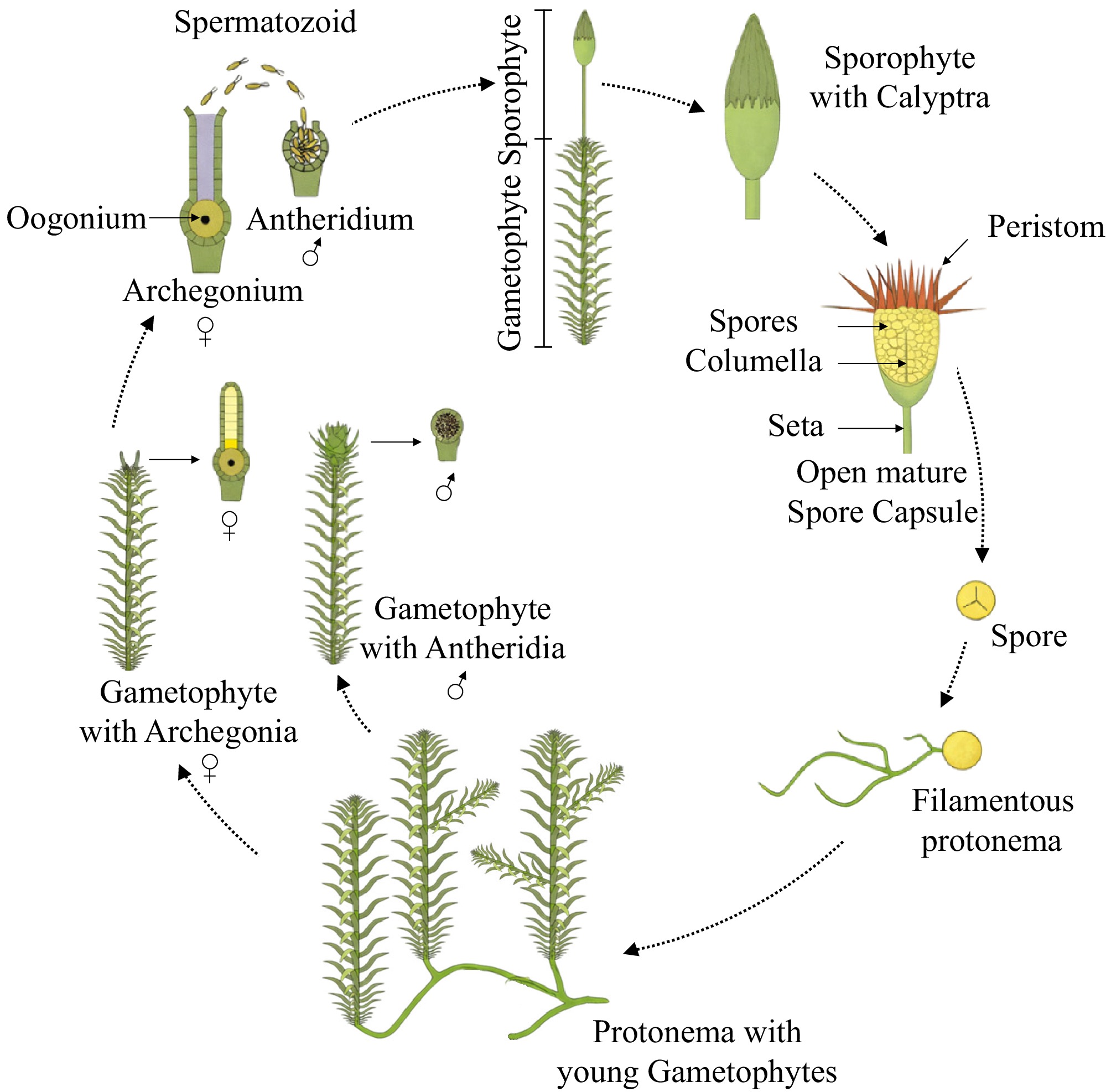
Figure 1. 

Generation cycle in peat moss; in photobioreactors, filamentous protonema and protonema with young gametophytes may occur, which are investigated here. The gametophytes carry small leaves and can develop side branches. The sprouting points at the ends are called capitula. Simplified tracing according to Dörken^[4].

It reproduces in the wild through spores, from which gametophytes grow. Like their algae ancestors, these are still adapted to submerged growth. For example, they can take up water and minerals through their whole surface and do not need roots. They drift in the water of the bog, eventually settle, and then form adult gametophytes. This haploid phase is then followed by a diploid phase, the sporophytes, which produce spores, closing the cycle. In higher plants, the diploid phase is the prominent form of the plant. It has now been shown that the gametophytes grow under submerged conditions while retaining their juvenile characteristics^[5]. High growth rates are achieved under sun or artificial lighting. These far exceed the growth rates of 0.2 day⁻¹ for adult plants in the bog. This makes the production of gametophytes in bioreactors the most effective way of mass propagation.

Growth in this context does not only mean an increase in biomass but also differentiation. On the macroscopic scale, one or several gametophytes form threads which eventually disintegrate, leading to a size distribution in the range of 0.3–5 cm. One order of magnitude below this, the single gametophytes show elongation of the filamentous parts, exhibit branching or the development of leaf structures. From especially metabolically active points, called "innovations", stems emerge, at the ends of which 'capitula' (heads) differentiate. After sowing, these stems transform into juvenile and finally separated adult gametophores.

To assess the progress of cultivation and optimize it by applying interventions in a PBR, using different light intensities or changing other environmental parameters, the gametophytes must be regularly examined and evaluated with respect to their morphological structure. In plant production, the content of bioactives is often of interest, but the low spatial resolution of such compounds is reported^[6]. For many purposes, morphological investigations are necessary. This can ideally be made by analyzing magnetic resonance (MR) images. A recent application for leaves as vegetative structure has been provided by Boulc'h^[7].

Magnetic resonance imaging (MRI) based on the detection of¹H nuclear spin signals (¹H-MRI) is an established noninvasive technique for investigating internal structures and physiological processes in living plants. Owing to the high natural abundance and mobility of hydrogen nuclei in water, ¹H-MRI enables spatially resolved visualization of hydration patterns, tissue organization, and internal transport pathways in intact organisms. Previous studies have successfully characterized water distribution, xylem and phloem transport, and three-dimensional (3D) root system architecture under hydrated conditions^[6,8−10]. Structural and functional analyses can be made without destructive sampling, thus allowing longitudinal studies on the same individual.

Beyond conventional high-field systems, ¹H-NMR (nuclear magnetic resonance) and MRI techniques have been adapted for in situ and mobile applications in plant research. Portable and unilateral low-field NMR sensors have been used to quantify water content and relaxation properties directly in intact plants^[11,12]. In addition, mobile ¹H-MRI systems have been demonstrated for use in greenhouses and in the field, enabling the nondestructive monitoring of hydration dynamics over extended periods without sample extraction^[13,14]. Advanced MRI techniques such as chemical exchange saturation transfer (CEST) imaging enable the indirect detection of low-concentration metabolites by exploiting ¹H exchange mechanisms, allowing the visualization of sugars and amino acids in vivo^[15]. Time-domain ¹H-NMR relaxometry and solid-state ¹³C-NMR have also been applied in peat and soil research to characterize pore structures, water-binding states, and organic matter composition^[16−18]. However, these studies primarily address bulk physicochemical properties and do not resolve the 3D morphology of living peat-forming plants.

Despite the ecological importance of peatlands and the central role of Sphagnum species in regulating water storage and carbon accumulation, the application of ¹H-MRI to the structural analysis of living peat mosses is largely unexplored. In contrast to vascular plants, bryophytes, particularly peat-forming mosses, have not been systematically investigated by 3D ¹H-MRI to resolve intact shoot architecture under hydrated conditions. Consequently, nondestructive quantification of morphological traits such as capitulum number, shoot density, or spatial organization within moss aggregates has not yet been established using MR methodologies.

The present study presents a ¹H-MRI-based workflow for the structural analysis of living S. palustre. Nondestructive 3D imaging allows for quantification of the morphological parameters, including the identification and enumeration of capitula within intact moss assemblages. This work establishes MRI as a tool for 3D structural phenotyping and growth assessment in peat moss cultivation systems.

Investigations were carried out on the strain S. palustre clone 12a (monoclonal) provided by the International Moss Stock Center and propagated at Albert-Ludwigs-University (Freiburg, Germany) in lab-scale bioreactors. The S. palustre biomass used for MRI analysis was cultivated at the Institute of Applied Biosciences and Process Engineering, Anhalt University, in 2-L bioreactors using an inorganic Sphagnum medium (composition according to study by Heck et al.^[19]) and 150 µmol·m⁻²·s⁻¹ incident light. The plants were kept at Karlsruhe Institute of Technology (Karlsruhe, Germany) in shaking flasks with illumination from the bottom.

MRI hardware and methods

MRI experiments were performed on an Avance Neo spectrometer equipped with a 9.4-T wide-bore superconducting magnet. The gradient system Micro2.5 was used in combination with a MicroWB40 MRI probe. An ¹H/¹³C-birdcage with an inner diameter of 25 mm was operated in linear mode on the ¹H channel.

Peat moss samples were positioned in 20-mm NMR tubes filled with water, thereby maintaining constant hydration throughout the measurement, and placed in the 25-mm MRI birdcage. Three-dimensional measurements were performed at room temperature, and the samples were stabilized to minimize motional artifacts. In addition, the imaging parameters were selected for contrast optimization and to avoid vibration-induced disturbances. Any sample movement would have resulted in visible image distortions or blurring; however, no such artifacts were observed in the acquired datasets. Potential biological growth during the 15.5-h acquisition period is expected to be negligible relative to the spatial resolution of the experiment (86 µm), and no growth-related structural changes were detected in the images.

Imaging was performed using the pulse sequence RARE (rapid acquisition with relaxation enhancement), which is based on the spin-echo principle^[20]. All experiments were performed within the software environment ParaVision 360 V3.5.

In the case of moss in water, the MR image contrast is primarily governed by differences in ¹H density as well as longitudinal (T₁) and transverse (T₂) relaxation times, which depend on the physical and chemical properties of primarily moss and water. The MR images were acquired under T₁ weighting, achieved by short repetition times (t_R) and echo times (τ_e). The main acquisition parameters are summarized in Table 1.

In T₁-weighted imaging, the signal intensity directly depends on the T₁. Materials with a short T₁, such as moss regions containing paramagnetic substances, exhibit high signal intensity, whereas materials with a long T₁, such as bulk water, yield lower signal intensity. Intensities are encoded in false color scales, which are provided together with the images. For visualization, the MATLAB® 'turbo' colormap was used. The displayed color scale (0–180) was chosen solely for visualization purposes and does not affect the underlying MR signal intensities. The MR images represent the measured signal amplitudes without additional normalization. The digital resolution of the signal amplitude was 32 bits. The contrast in the images enabled a clear identification of the moss within its aqueous environment.

Approaches for detection and evaluation of structures

The MR images of the gametophytes were analyzed using a pattern recognition approach consisting of two stages: Feature extraction and classification in feature space. 'Matched filters' were used specifically for feature extraction. In this process, a morphological detail to be identified in the MR images was reproduced in the computer as a digital model. The smaller model matrix was then moved over the much larger observation matrix and the scalar product was formed at each location. The better that the structures of the filter and the measured data matched, the higher the values of this moving scalar product. A common application in the field of time signals is the automated evaluation of long-term electrocardiograms (ECGs) by storing various forms of typical waves. In the present case, a 3D matrix MF(x,y,z) was formed as a matched filter. The cross-correlation (CR) with the measurements, i.e., the observation space OS(x,y,z), is then

The calculation was carried out in MATLAB using the routine 'convn'. The maximum value of CR was obtained for the displacement (u, v, w) at which the greatest similarity between the filter structure and a region in the MRI image occurred. In a second step, a decision was made about the actual presence of a (parameterized) search object and clustering is performed. The decision about belonging to a cluster was made on the basis of a threshold to be determined in the feature space, i.e., the height of the filter response.

Clustering or, more precisely, 'segmentation' is performed using the K-means algorithm^[21]. This algorithm finds k different points named centroids c, minimizing the Euclidean distance of all members of the observation space to their specific centroid, then the data points are assigned accordingly and c is adjusted dynamically as the mean value. This approach does not contain enough information for the type of biological segmentation given here. Therefore, feature space augmentation is necessary. This is done by using the signal amplitude of each data point and minimizing the difference of this feature to its centroid. The two aspects, shown as the two terms in the sum of the cost functional, are controlled by the weighting factor w. In this way, similar direct neighbors are likely to belong to the same segment.

For the appropriate calculations, the MATLAB routine 'imsegkmeans3' was used. This makes leaves, for example, with a contiguous group of voxels distinguishable from structures with similarly high signal values. At the end of the iterative optimization, all voxels are assigned to distinct segments.

In order to obtain optimal MRI settings and to enable the detection of individual morphological characteristics, gametophytes from different stages of cultivation were selected. Typical features were compared using light microscopy and MRI, as shown inSupplementary Figs. S1−S3. The gametophytes in the bioreactor typically had filamentous, flexible stems with a capitulum and lateral branches (Supplementary Fig. S1a). Thalloid structures were found at the base and as leaflets on the stems and lateral branches. It has not yet been investigated whether the gametophytes in turbulent bioreactors grow differently from gametophytes in bogs, where only slow drift may occur.

To provide material for investigation, the threads were maintained in bottom-lit shaking flasks while being moderately shaken. The stems grew downward toward the light (Supplementary Fig. S1b). This suggests that the gametophytes have little or no perception for gravity under water. S. palustre gametophytes do not have rhizoids, whereas other moss species have been shown to have gravireceptors in the rhizoids.

To observe the differentiation into adult gametophytes, material from the reactors was planted out on peat substrates (Supplementary Fig. S1c). Here, the structure with a vertical stem and the characteristic pattern of branches developed (Supplementary Fig. S2). Microscopic images for comparison can be found in study by Müller et al.^[22]. In addition, they could absorb nutrients from the water, a trait they inherited from algae as their ancestors.

A gametophyte that has already developed significantly into a young adult plant (Supplementary Fig. S2a) already exhibits clearly defined lateral branches.

The leaves on the stem are arranged in a spiral pattern. The side branches emerge from the leaf spines of the stems. They grow at constant intervals of the leaf rings, resulting in a regular pattern (Supplementary Fig. S3). The gametophyte of S. palustre can have single spines (side branches) but also paired spines that are pendant and divergent. In the adult phase, the pendant branches hang down along the stem, contributing to the capillary movement of water. The divergent branches stick out from the stem. The leaves at the spines are different from the leaves of the stem^[23].

Measures for quantitative visual inspection

To assess the progress of cultivation, the effects of interventions in the PBR and process control, as well as the growth behavior, the gametophytes must be regularly examined and evaluated quantitatively. Optical inspection by four-dimensional light-field methods is possible, but it requires manual processing to avoid mutual concealment and it cannot be considered reliable. For the planned decentralized production, it will be practically impossible. This section aims to show that automated quantitative analysis is possible with 3D MRI images with the inherent advantage of a nondestructive and noninvasive analysis of optically opaque samples as well.

A specimen of a gametophyte was chosen as an example, which was used for seeding on peat for two weeks after cultivation in the reactor. It already shows some differentiation patterns. In a first step, improved visibility for human examiners is a practical goal. The images in Fig. 2 show representations of the 3D view from four different angles. The example indicates the number of capitula and the amounts of leaflets. The number of side branches, the total amount of biomass and, if possible, its composition are relevant parameters. For the inspection of signal intensities, the individual voxels are color-coded as shown in the color bar in Fig. 2.

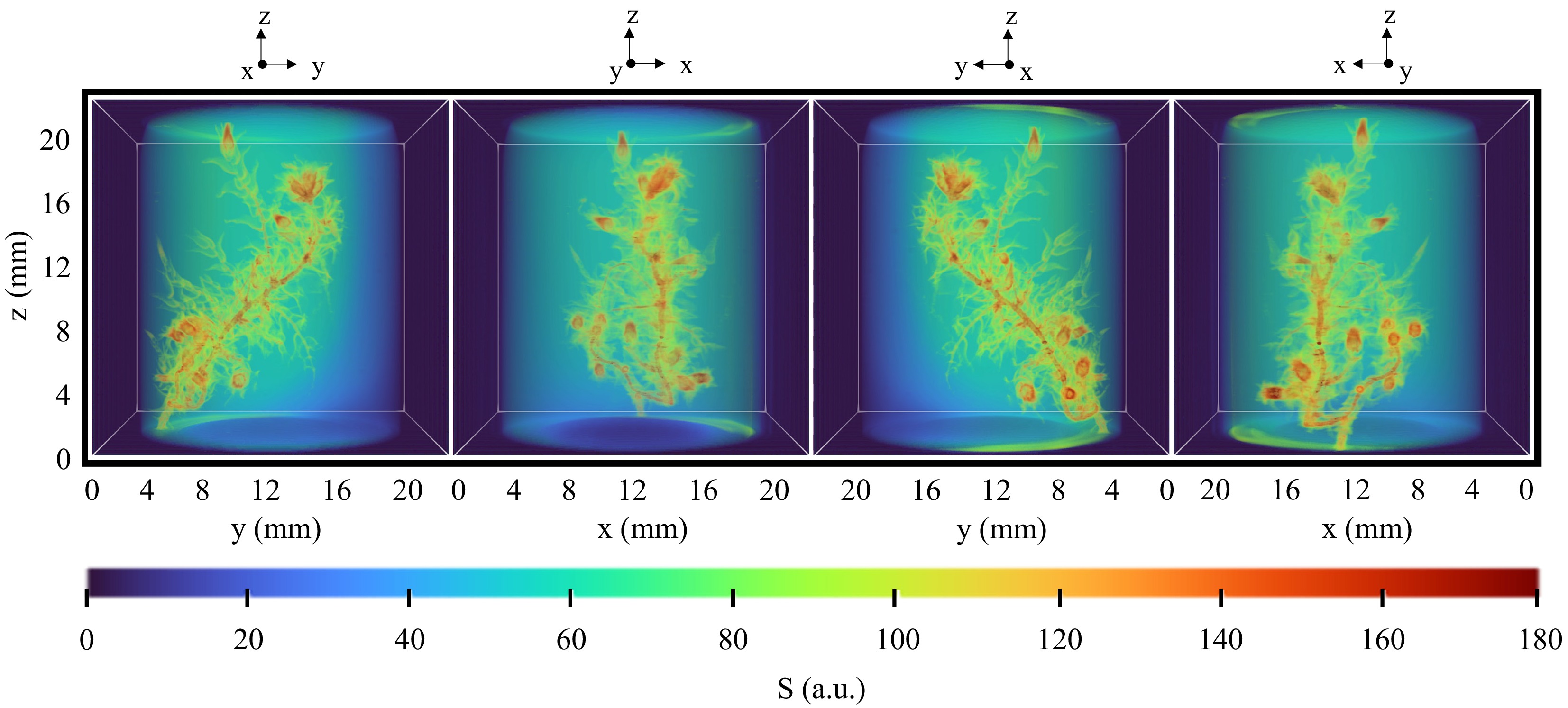
Figure 2. 

A specimen of a gametophyte chosen as an example; the images show four different views of a 3D MRI dataset consisting of 256 × 256 × 256 voxels. The cylindrical structure is a signal from the sample vial. The color bar, 'turbo' in MATLAB, gives the code for the signal intensities between 0 and 180 corresponding to the highest measured value in this set. The colors follow the sequence in a visible light spectrum from blue to red. Capitula and stems appear in orange-reddish colors, whereas leaves and water-rich regions appear in yellow-green with reduced signal intensities caused by T₁ weighting.

The specimen is a typical gametophyte with a central filament that curves downward at the bottom of the vial and grows upward again. Furthermore, larger side branches can be seen in both the upper and lower parts. All filaments are densely covered with leaflets (green) and end in capitula. Both the central filament axes and the capitula show a moderately higher signal (orange) than the leaflets. The reason for this is that these structures have a denser biomass packing, whereas the leaflets consist of only one cell layer containing additional water-filled hyalocytes. In these views, a qualified inspection of the samples is already possible.

To further improve interpretation and quantification, the first measure is to crop the region of interest (here, this is the biological object) from the background. In this case, this means reducing the observation space to the interior of the tube. This is achieved by setting voxels outside the cylindrical structure to zeros or NaN. However, Supplementary Fig. S4 shows that a clear view is only possible in slices through the structure, unless the water background is made transparent.

For further improvement, a second measure is to search for sections in the intensity density distribution that enable selective mapping. The results are given in Supplementary Fig. S5. The histograms are calculated from the voxel signal intensities, which are not transparent. Exact numbers are given in the figure captions.

The structure in the signal intensity range from 30 to 80 can mainly be attributed to the water body. Interestingly, this structure is approximated well by a three-mode Gaussian function. To get a clear 3D image of the moss, voxels with a signal intensity < 80 (i.e., water regions) are made transparent, thus allowing a clear view of the plant (Fig. 3). This procedure is also useful to identify objects with respect to their signal intensity.

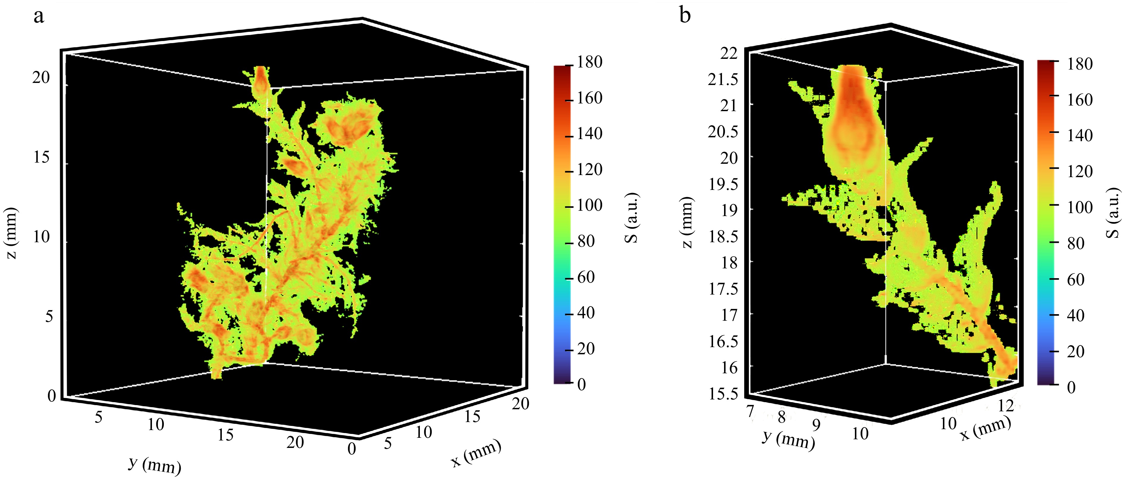
Figure 3. 

A 3D segmented MR image of the clipped gametophyte. Signals from the vial and the water are cut off. Now it can be investigated in its full information content. (a) Clipped gametophyte; no disturbing additional signals are to be seen. (b) Clipped capitulum; the leaflets are somewhat disturbed, as some parts (edges) are not fully covered by one voxel and therefore the signal intensities are too close to that of the surrounding water.

Such measures do not increase the information content but make fast inspection easier and reduce the error rate of automated signal filters and image analysis. In the view shown in Fig. 3, it would, in principle, be possible to count the innovations and side branches while manually interacting with the volume view on the screen. To get a better identification and a higher degree of automation, different methods of pattern recognition were applied.

Approaches for quantitative analysis

Automatic analysis of the samples in terms of morphological characteristics is crucial. The advantage of this computer-assisted automation lies in its greater accuracy, reproducibility, and, above all, lower costs compared with the manual approach. We can apply a 3D matched filter. In the first stage of this process, a test pattern is defined. An ideal digital model of a capitulum would work well^[24]. The problem here, however, is that the capitula to be counted are all slightly different. Therefore, a model is needed that simplifies a larger range of objects to be searched for. For the sake of simplicity, a simple sphere was chosen as the prototype of a sample and thus for the central part of the filter (Fig. 4a). This overlaps a large part of the slightly different capitula. Further, no runs with different angles between the pattern and the observation space are necessary, although the capitula can show with their openings in all different directions. The distribution of filter responses is shown in Fig. 4b.

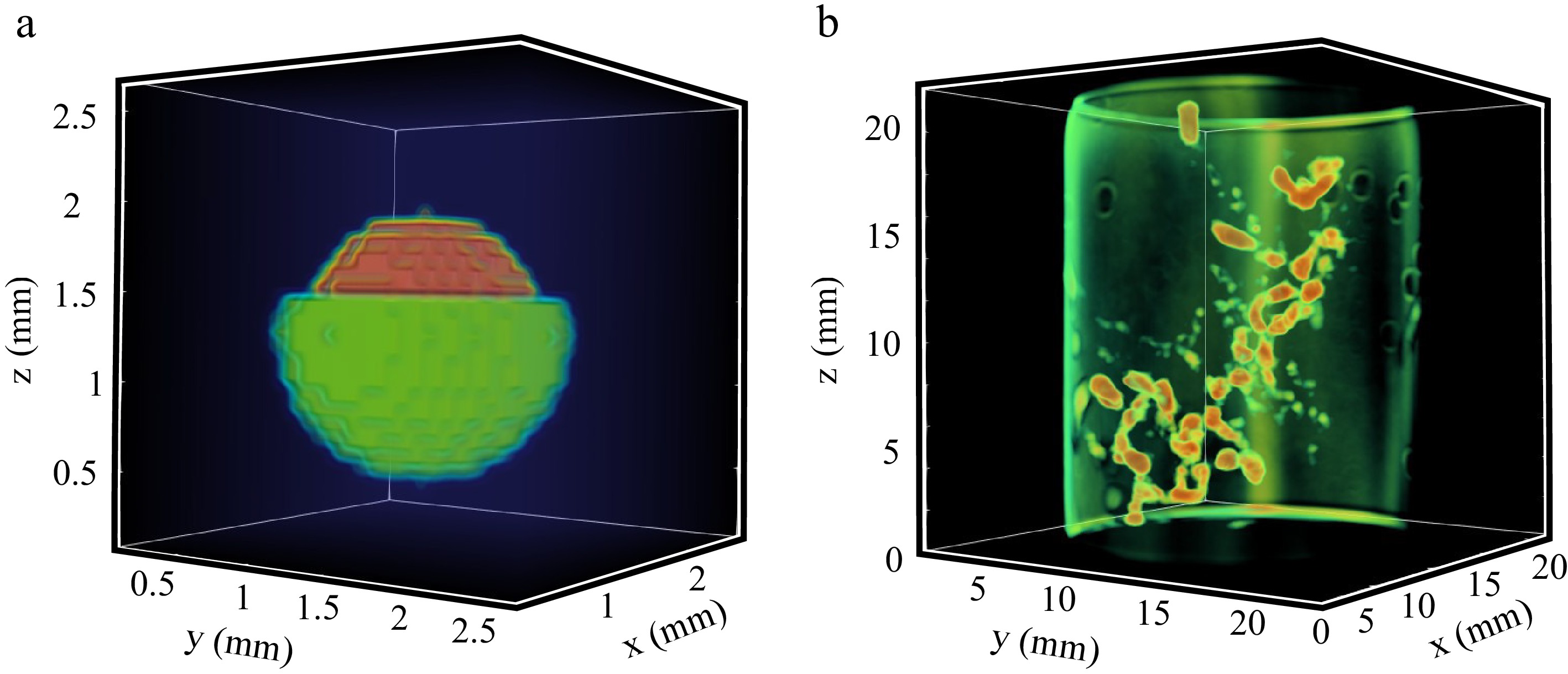
Figure 4. 

Volume view of the structure of the matched filter and the filter response; capitula are clearly separated from leaves and from the background. (a) Cutaway diagram of the pattern volume; it is a sphere (red) with a radius of 8 voxels. The rough surface structure reflects the approximation of the sphere with cubic voxels. The coating (green) is 2 voxels thick and the cubic matrix (blue) has an edge length of 31 voxels. (b) The cross-correlation response function clearly shows the capitula as the most intense structures. Background and leaves are nearly completely suppressed, while stems are only partially suppressed.

The matching sphere has a positive weighting factor in the matrix multiplication. It is covered by a coating with negative numbers to bring the mean value to zero. This is actually necessary to suppress constant areas with high signal amplitudes. In addition, the observation matrix as a whole is normalized to a mean of zero and an average absolute height of one. As matrices are usually defined to be rectangular, the actual filter structure is embedded into a cubic matrix filled with zeros. The highest value observed is 8,000 a.u. The complete probability density function is shown in Fig. 5a.

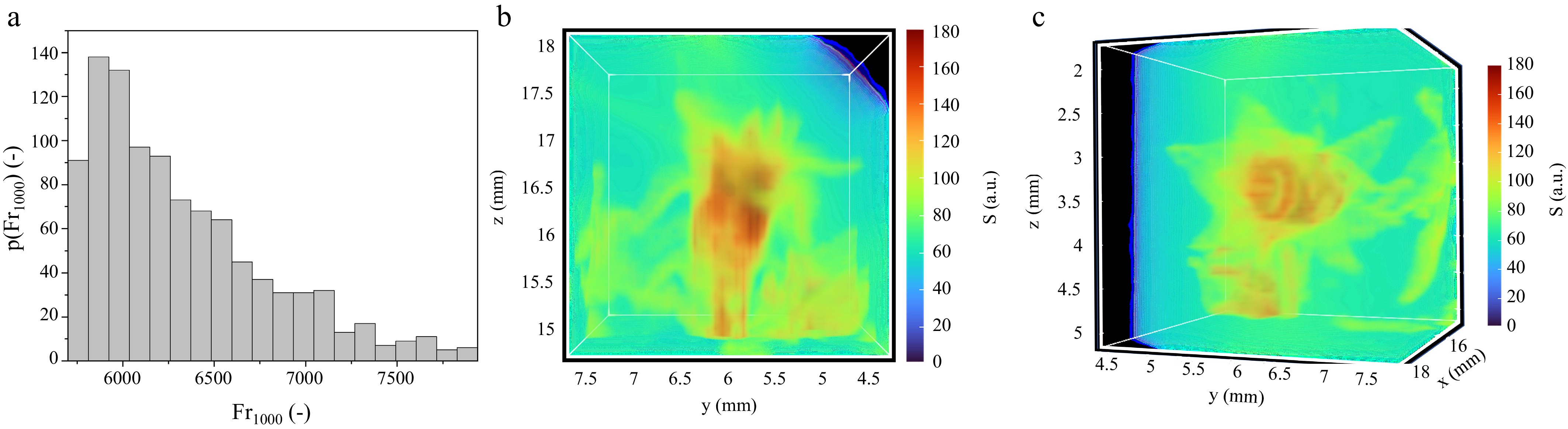
Figure 5. 

Distribution density of the filter response and detailed view of the capitulum with the highest matched filter response. (a) Number/size distribution of the largest 1,000 filter responses; starting from the highest value, the hits were clustered by direct neighborhood resulting in ~17 locations of capitula, depending on the fixed threshold. (b) An identified capitulum in detail, namely the one with the highest response; the cube has an edge length of 40 voxels, which corresponds to 1.2 mm. (c) In the view looking down on the capitulum from above, the capitulum is open at the top like a chalice.

The second block in the filter approach is the decision block. This can generally be done by setting a threshold above which a high value in the filter response is classified as a capitulum. However, the filter also generates high values in its transient responses, so several neighboring global maxima must be classified together as one hit. The classification was performed on all of the 1,000 highest filter responses. Starting from the highest value, all smaller maxima closer than 2 voxels to an already assigned maximum were clustered together with this maximum. The whole cluster marks a capitulum. The remaining values were then treated in the same way. A minimum value of 6,000 a.u. was defined for the value of a valid cluster. Smaller values have been found to be small growing points without the development of a full capitulum structure. The decision is not clearly defined in reality or under personal inspection. Therefore, the reduction in the size distribution density function (the lowest bar on the left) was taken as a reproducible value. An exclusion threshold for small capitula can also be selected by using a visually defined small filter response as the boundary. Seventeen capitula were finally discovered in this way, which corresponds to the number that was reliably counted (Fig. 4b) beforehand.

To determine the leaf mass, the clustering algorithm 'imsegkmeans3' in MATLAB was used. This algorithm evaluates not only the intensity of data points but also their similarity to their nearest neighbors. The algorithm found three clusters k = 3 (Fig. 6) without user specification. This decision was made by the algorithm on feature (spatial and color) distances. Actually, this meets the expectations, as the first cluster refers to the nonspecific environment (water), the second to the leaf biomass, and the third to the parenchyma inside the stems and twigs as well as inside the heads. The number of neighbors was significantly lower in the leaves than in the parenchyma because of their single-layer structure. The neighborhood factor is therefore decisive.

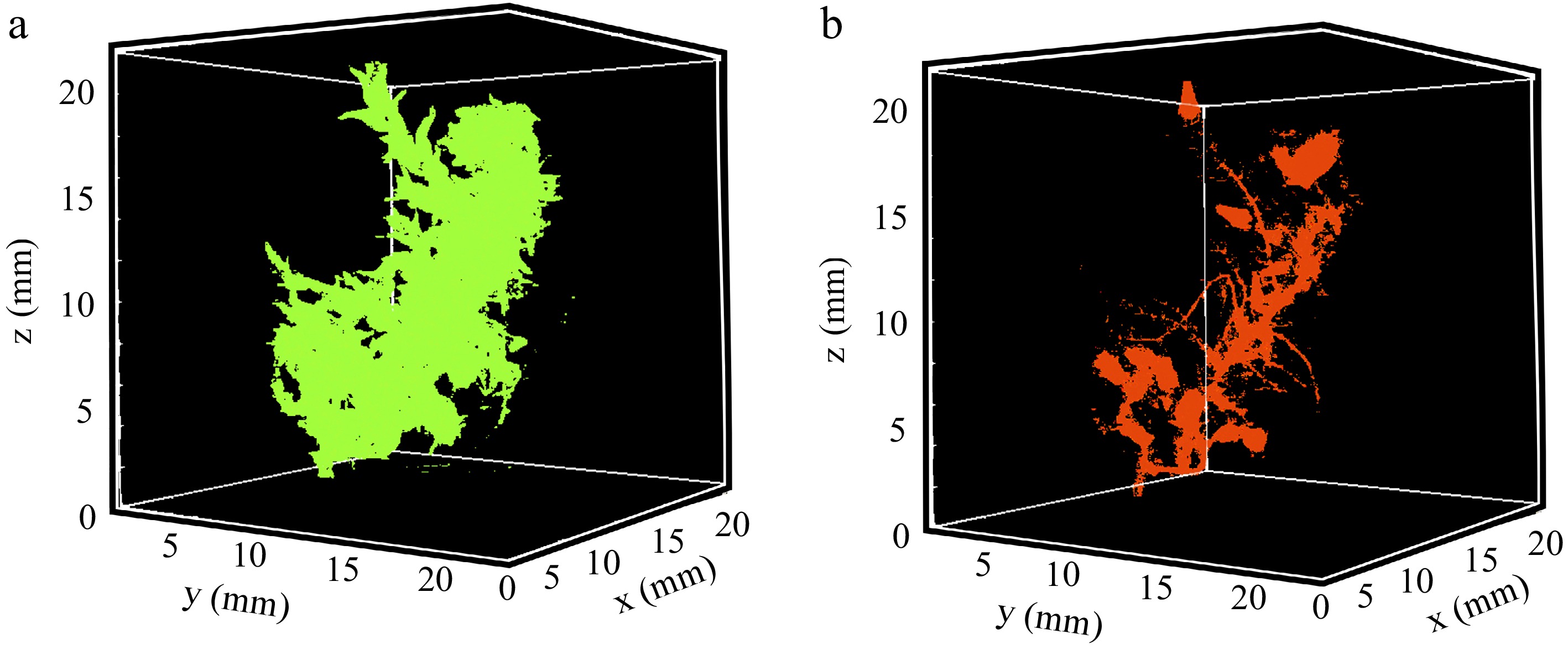
Figure 6. 

The three segments after segmentation; against the background as one segment in black, the algorithm found an outer segment, shown here in green, and an inner segment in red. (a) Segment No. 2 in green represents the foliage of the plant. As one would expect from a biological process, the segment forms a continuous volume. (b) Segment No. 3 in red represents the stems and capitula. Leaves are intentionally left out by the algorithm.

To show that the parenchyma segment is definitely surrounded by the leaf segment, cross-sections are shown in Supplementary Fig. S6. The inner segment is definitely completely covered by the outer segment.

To give a final assessment of the performance of the algorithms, both segment volumes and the capitula detected from the matched filter are shown in Fig. 7 as an overlay, with the leaf segment made slightly transparent.

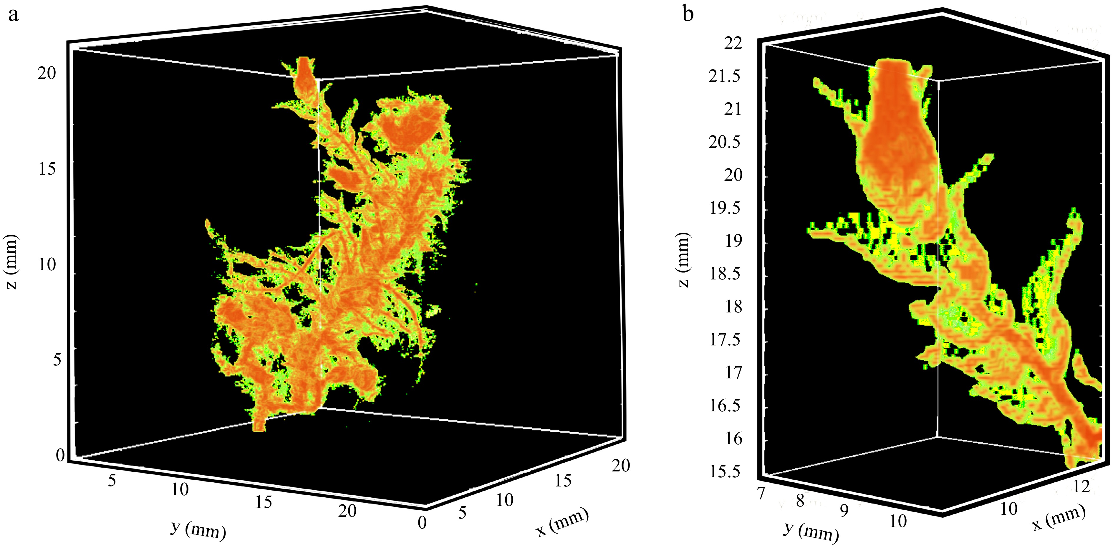
Figure 7. 

Results of the quantitative analysis of the preparations using clustering based on a k-means algorithm. The outer (green) segment is made half-transparent to make the inner structure visible. (a) Both clusters showing the plant material together. There is a clear correlation between the material of the stems and the leaf material. (b) A detailed view of the clusters showing the capitulum with the highest filter response of the preparation; the perforated structure of the leaves is caused by the limited spatial resolution, i.e. the interference of leaf edges with the voxel structure.

All voxels were detected and assigned to a specific cluster called a 'segment'. Even the background was properly assigned. From the approximate 120,000 voxels counted, about 70% were assigned to leaves, which is the first measure for the biomass share. One reason for any inaccuracies is that the edges of the leaves can only partially overlap with a voxel and therefore show only low intensities, a fact known in MRI as the partial volume effect. This can effectively be circumvented by a higher resolution in the range of 10 µm.

Investigation of plants using MRI is established as a means in botanical research, e.g. to measure ingredient contents. In this paper, MRI analysis was successfully applied to detect morphological changes during plant development. For image analysis, matched filters and the k-means algorithm were successfully applied. These methods are well-established tools in pattern recognition and form part of the methodological foundation of many modern data analysis frameworks. The results show that MR images' intensity distributions contain relevant information that reflects key physiological and morphological properties of the gametophytes and can be used for straightforward quantitative evaluation.

Beyond methodological aspects, the presented approach provides a basis for automated monitoring of moss cultivation processes. This is particularly relevant for large-scale or decentralized bioreactor systems, where manual inspection is not feasible. In this context, MRI-based analysis may contribute to control and optimization of the process, for example, by enabling the assessment of structural development under varying growth conditions.

Moss cultivation is increasingly considered for applications beyond ecological restoration, including the production of biomaterials and biotechnological products such as recombinant proteins in established Sphagnum-based expression systems^[25]. The ability to nondestructively quantify its morphological development therefore supports both ecological and biotechnological applications.

Future developments may integrate MRI acquisition with machine learning approaches to enable automated and potentially real-time analysis of plants' structure and growth dynamics in complex bioprocessing environments.

The procedure of MRI measurements and data processing has been shown for the example of propagating moss gametophytes (Sphagnum) in PBRs. This approach could effectively contribute to the quality assessment of gametophytes, where, for example, the number of capitula is decisive for planting success. The significance of the MRI-based approach reported here could also be extended to other bioprocesses with spatially differentiated biomass, e.g., pellet formation or organisms with filamentous structures. Further development of smart devices for MRI in combination with artificial intelligence for image analysis could open a new dimension for developing bioprocesses.